Temporal Stability of Soil Moisture and Radar Backscatter Observed by the Advanced Synthetic Aperture Radar (ASAR)

Abstract

The high spatio-temporal variability of soil moisture is the result of atmospheric forcing and redistribution processes related to terrain, soil, and vegetation characteristics. Despite this high variability, many field studies have shown that in the temporal domain soil moisture measured at specific locations is correlated to the mean soil moisture content over an area. Since the measurements taken by Synthetic Aperture Radar (SAR) instruments are very sensitive to soil moisture it is hypothesized that the temporally stable soil moisture patterns are reflected in the radar backscatter measurements. To verify this hypothesis 73 Wide Swath (WS) images have been acquired by the ENVISAT Advanced Synthetic Aperture Radar (ASAR) over the REMEDHUS soil moisture network located in the Duero basin, Spain. It is found that a time-invariant linear relationship is well suited for relating local scale (pixel) and regional scale (50 km) backscatter. The observed linear model coefficients can be estimated by considering the scattering properties of the terrain and vegetation and the soil moisture scaling properties. For both linear model coefficients, the relative error between observed and modelled values is less than 5 % and the coefficient of determination (R²) is 86 %. The results are of relevance for interpreting and downscaling coarse resolution soil moisture data retrieved from active (METOP ASCAT) and passive (SMOS, AMSR-E) instruments.

1. Introduction

Soil moisture is highly variable in space and time. Soil moisture patterns are spatially organized phenomena, influenced by geology and topography, land cover and climate [1]. Within a few meters soil moisture can vary as much as within a distance of kilometres [2]. In the temporal domain the soil moisture of the top part of a soil profile, which is directly exposed to the influences of the atmosphere, can vary significantly over hours [3]. Several studies showed that soil moisture variations in space and time can be related to a small scale and a large scale component [4]. The small scale component leads to local variations in soil moisture due to soil properties, land cover attributes and local topography. This small scale component acts in the range of tens of meters spatially and in the range of a few days temporally [5]. The large scale component is related to atmospheric forcings, namely precipitation and evaporation processes. Based on extensive in-situ data sets in Russia, Vinnikov et al. [6] observed spatial correlation lengths of soil moisture in the order of 400 – 800 km caused by atmospheric forcing. These findings are supported by [4] reporting spatial correlation lengths in the order of several hundred kilometres for test sites in Russia, Mongolia, China and Illinois, USA.

As a result of large scale atmospheric forcing, temporal soil moisture variations can be expected to be similar across different spatial scales, from meters to hundreds of kilometres. At local scale these atmospheric-driven temporal variations are modulated by small-scale hydrologic processes related to terrain, soil, and vegetation characteristics. Experimental work based on in-situ soil moisture measurements has demonstrated that spatial soil moisture patterns tend to persist in time and that therefore soil moisture measured at single in-situ stations is often highly correlated with the mean soil moisture content over an area. This observation has been exploited by the temporal stability concept proposed by Vachaud et al. [7] to identify stations that have a similar absolute value and temporal trend as the mean soil moisture content over an area. In other words, temporal stability of spatial soil moisture patterns allow one to estimate the areal mean soil moisture from point measurements. Conversely, it should be possible to go the opposite way to estimate local scale soil moisture from areal measurements delivered by remote sensing.

The questions of whether, where and how coarse resolution satellite data can be used at finer scales are important because, within the next few years, only coarse resolution (25-50 km) soil moisture data derived from spaceborne radiometer and scatterometer systems can be expected to be operationally available [8]. Global soil moisture products are already available from the Advanced Microwave Scanning Radiometer (AMSR-E) [9] and from the Advanced Scatterometer (ASCAT) onboard of the Meteorological Operational (METOP) satellite series [10]. The Soil Moisture and Ocean Salinity (SMOS) satellite is planned to be launched in 2008 [11]. The spatial resolution is 25 km for ASCAT, 43 km for SMOS, and 56 km for AMSR-E (C-band). For soil moisture retrieval at finer spatial scales, Synthetic Aperture Radar (SAR) may be used. However, scientific and technological breakthroughs are still needed for the operational use of SAR [12].

Given that soil moisture has an important influence on radar backscatter measurements at all spatial scales, it is hypothesized that temporally stable soil moisture patterns lead to temporally stable radar backscatter patterns. To verify this hypothesis, long-term backscatter time series acquired by the Advanced Synthetic Aperture Radar (ASAR) flown on board of the European satellite ENVISAT are analysed in this paper. ASAR can be operated in Wide Swath (WS) mode to cover a much wider swath (swath width of 405 km) than in conventional strip-map mode (swath width of 100 km). In this way, large areas can be more frequently imaged and long backscatter time series can be more easily constructed.

2. Theory

2.1. Temporal Stability of Soil Moisture

The concept of temporal stability was introduced by [7] as a practical means of reducing a large ground-based soil moisture measurement network to a few representative sites. On a more fundamental level, the temporal stability concept is important because it suggests that spatial soil moisture patterns persist in time. The existence of time stability was confirmed by many studies [13], although hydrological processes such as topographically driven lateral redistribution of soil moisture may create a lack of time stability [14].

Let us consider a soil moisture network with n measurement sites. The mean soil moisture content over the region, θ_r, at time t_j is estimated by

$${\theta }_r\left(t_j\right)=\frac{1}{n}\sum _{i=1}^n{\theta }_p(x_i,y_i,t_j)$$

(1)

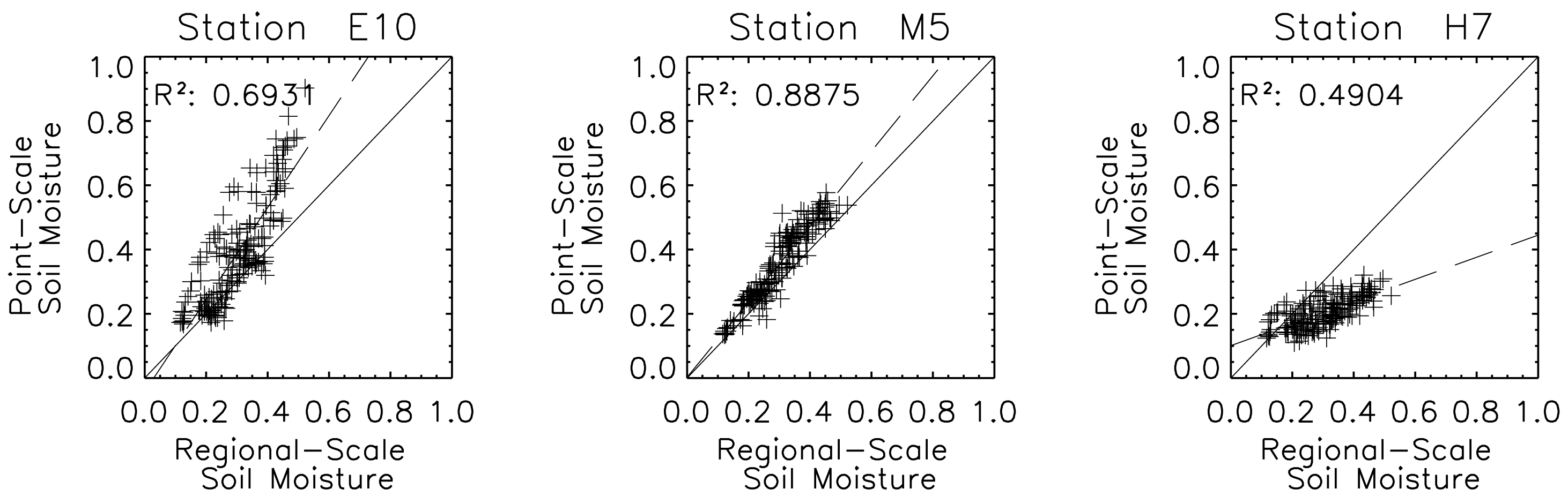
where θ_p is an in-situ soil moisture measurement at point with coordinates (x_i, y_i). The measurement scale of the in-situ sensors is denoted here as point scale because the measurements are only representative of a small area ranging from about 0.1 to 10 dm² depending on the employed measurement technique (see [15] for a discussion of different in-situ measurement techniques). For identifying the most representative soil moisture stations [7] used the relative difference between point scale and regional scale soil moisture

$${\delta }_{i,j}=\frac{{\theta }_p(x_i,y_i,t_j)-{\theta }_r\left(t_j\right)}{{\theta }_r\left(t_j\right)}$$

(2)

and calculated the mean and standard deviation of δ_i,j over time. While the mean of δ_i,j informs us if location (x_i, y_i) is in general drier, wetter or about the same as the regional soil moisture value, the standard deviation of δ_i,j tells us how well θ_p reflects the temporal trend of θ_r. Low values of the standard deviation of δ_i,j indicate a high time stability of the spatial soil moisture patterns, implying a strong correlation of point scale and regional scale soil moisture time series. Temporal stability can thus also be assessed using the temporal correlation coefficient between point scale and regional scale soil moisture [16, 17]. For example, Cosh et al. [13] found that the temporal correlation (R²) of station soil moisture with the regional mean over the 610 km² Little Washita Watershed located in Oklahoma, USA, was larger than 0.75 for the majority of the sites. Grayson and Western [14] found R² values of more than 0.9 in the 10.5 ha Tarrawarra catchment near Melbourne, Australia.

Given temporally stable soil moisture patterns, time-invariant relationships can be used for estimating regional soil moisture θ_r from point scale measurements θ_p, a process commonly referred to as “upscaling”. De Lannoy et al. [18] tested different upscaling methods at a 21 ha site situated in Maryland, USA, and found that a simple linear relationship provided good results. This observation was also made by Baup et al. [19] at a 1 km² large Sahelian site located in the Gourma region in Mali. Not only in in-situ measurements but also in hydrologic simulations such relationships have been observed. For example, [20] investigated the temporal stability of soil moisture patterns at different spatial scales using hydrological model simulations for a mesoscale catchment (75000 km²) and found that a linear model was well suited to describe the relationship between 1 km² and 40 × 40 km² soil moisture fields. One can hence write

$${\theta }_r\left(t_j\right)=c_{\mathit{\text{rp}}}(x_i,y_i)+d_{\mathit{\text{rp}}}(x_i,y_i){\theta }_p(x_i,y_i,t_j)$$

(3)

where c_rp and d_rp are location specific coefficients that depend on the soil, topography and vegetation. The subscripts of the two coefficients indicate the two scales and their sequence indicates the direction of scaling (from point to regional scale). The coefficients c_rp and d_rp can be estimated for each site within a soil moisture network area, whereas the suitability of this linear model can be expressed in terms of the correlation coefficient and the standard error of estimate (SEE).

Instead of confining Equation (3) to a few sample points within a measurement network, it is now applied to any arbitrary point (x, y) situated within a region $ℛ$ of size A_r:

$${\theta }_r(t)=\frac{1}{A_r}\underset{ℛ}{\iint }{\theta }_p(x^{\prime },y^{\prime },t){\mathit{\text{dx}}}^{\prime }{\mathit{\text{dy}}}^{\prime }=c_{\mathit{\text{rp}}}(x,y)+d_{\mathit{\text{rp}}}(x,y){\theta }_p(x,y,t)$$

(4)

In subareas of region $ℛ$ where large-scale atmospheric forcing has a dominant control on soil moisture, the upscaling model (4) is expected to give good results. On the other hand, at points (x, y) dominated by small-scale hydrologic processes (e.g. high groundwater tables) the relationship is expected to be poor. By re-arranging Equation (4) one obtains the downscaling equation

$${\theta }_p(x,y,t)=c_{\mathit{\text{pr}}}(x,y)+d_{\mathit{\text{pr}}}(x,y){\theta }_r(t)$$

(5)

where the reverse sequence of the subscripts now indicates that the soil moisture content at point (x, y) is estimated from the regional value θ_r. The downscaling coefficients c_pr and d_pr are related to the upscaling coefficients c_rp and d_rp by:

$$c_{\mathit{\text{pr}}}=-\frac{c_{\mathit{\text{rp}}}}{d_{\mathit{\text{rp}}}}$$

(6)

$$d_{\mathit{\text{pr}}}=\frac{1}{d_{\mathit{\text{rp}}}}$$

(7)

Estimates of the regional soil moisture content θ_r at time t may come from remote sensing or from soil-vegetation-atmosphere transfer models. If, additionally, spatially explicit estimates of the coefficients c_pr and d_pr are available, then it is possible to infer small-scale soil moisture patterns using the downscaling Equation (5).

2.2. Temporal Stability of Radar Backscatter

Over bare soil and moderately vegetated terrain, radar backscatter is sensitive to soil moisture. In such areas it can be expected that the temporal persistence of soil moisture patterns is reflected in the spatio-temporal behaviour of the radar backscattering coefficient. For a better quantitative understanding of this effect, a model relating backscatter across two spatial scales is derived in the following.

Radar backscatter from land surfaces is a complex function of sensor parameters (frequency, polarization, incidence angle) and external factors given by the dielectric (soil moisture, vegetation water content) and geometric (surface roughness, plant structure) properties of the imaged terrain [21]. Backscatter from rough soil surfaces and vegetation canopies can be modelled starting from Maxwell's equations [22, 23]. Unfortunately, many of the available theoretical models have failed to produce results that are in good agreement with observations, as discussed for the case of bare soil backscatter models by [24-26]. In contrast, simple change detection techniques have provided more promising soil moisture retrievals as an extensive review of microwave remote sensing methods for soil moisture retrieval has shown [12]. Fortunately, such change detection models are sufficient for the discussion of temporal stability patterns because only the temporal variability of the radar signal needs to be explicitly modelled for that purpose.

Change detection methods rest upon the idea that reference images representing dry soil conditions are subtracted from each radar image to implicitly account for surface roughness and land cover patterns [27, 28]. One formulation of the change detection method is [29]:

$${\sigma }^0(x,y,t)={\sigma }_{\mathit{\text{dry}}}^0(x,y,\overline{t})+S(x,y,\overline{t})\theta (x,y,t)$$

(8)

where σ⁰_dry is the backscattering coefficient observed under completely dry soil conditions expressed in decibels, and S is the sensitivity of the backscattering coefficient σ⁰ to changes in soil moisture θ. In change detection, the soil moisture content is conveniently expressed in terms of the degree of saturation which is the volume of water present in the soil relative to the volume of pores [30]. It ranges from zero in dry soil to unity (or 100 %) in a completely saturated soil. The two parameters σ⁰_dry and S depend on surface roughness and vegetation conditions. σ⁰_dry typically increases with increasing surface roughness and vegetation biomass and S decreases with increasing vegetation opacity. While S generally varies over time reflecting changes in vegetation phenological state, surface roughness is generally assumed to be constant.

While soil moisture θ may vary within minutes to hours due to rainfall, the backscatter parameters σ⁰_dry and S vary in general more slowly in the order of days to months reflecting changes in vegetation phenology. Therefore, within time periods [t−Δt/2, t+Δt/2] of duration Δt, σ⁰_dry and S may in a first approximation be treated as constants. To remind us of the much slower temporal variability of σ ⁰_dry and S compared to θ and σ⁰, the time t within the brackets of σ⁰_dry and S was written as t̅ in Equation (8). This notation only serves to facilitate the interpretation of equations derived in the following, but has no implications from a physical point of view, i.e. t̅ = t. The implication of treating σ⁰_dry and S as constants within a time period [t−Δt/2, t+Δt/2] is that phenomena occurring within this time period and having a strong effect on σ⁰_dry and S appear as “noise”. Examples for such noise-like effects are farming activities such as harvesting or ploughing which lead to rapid changes in σ⁰_dry and S, particularly at small scales.

The change detection model (8) has successfully been applied to coarse-resolution (50 km) ERS scatterometer measurements on a global scale [31]. Several validation studies have confirmed its applicability to different climate- and vegetation zones [32-35]. At finer spatial scales, [36] used this model to retrieve 1 km soil moisture maps from ENVISAT ASAR Global Monitoring (GM) images over the southern African continent. Change detection approaches have also been successfully applied to airborne radar measurements, such as recently demonstrated for L-band airborne radar observations acquired during the 1999 Southern Great Plains (SPG99) experiment [37] and the 2002 Soil Moisture Experiment (SMEX02) [38].

For the discussion of spatio-temporal trends two spatial scales are considered, one denoted by local scale and one by regional scale. The local scale is represented by an area $ℒ$ of size A_l which is chosen here to be the pixel size of a Synthetic Aperture Radar (SAR) image. The regional scale is, as before, represented by the region $ℛ$ of size A_r. It is assumed that the region $ℛ$ is much larger than the local area $ℒ$, i.e. A_r ≫ A_l. The change detection model given in Equation (8) is now applied at both scales:

$${\sigma }_l^0(x,y,t)={\sigma }_{\mathit{\text{dry}},l}^0(x,y,\overline{t})+S_l(x,y,\overline{t}){\theta }_l(x,y,t)$$

(9)

$${\sigma }_r^0(t)={\sigma }_{\mathit{\text{dry}},r}^0(\overline{t})+S_r(\overline{t}){\theta }_r(t)$$

(10)

where the subscripts l and r indicate the spatial scales of the different variables. Equations (9) and (10) can be coupled if a relationship between local and regional scale soil moisture can be established. The mean soil moisture content of the local area $ℒ$ centered at the coordinates (x, y) is given by

$${\theta }_l(x,y,t)=\frac{1}{A_l}\underset{ℒ}{\iint }{\theta }_p(x^{\prime },y^{\prime },t){\mathit{\text{dx}}}^{\prime }{\mathit{\text{dy}}}^{\prime }$$

(11)

By substituting the downscaling Equation (5) into (11)

$${\theta }_l(x,y,t)=\frac{1}{A_l}\underset{ℒ}{\iint }(c_{\mathit{\text{pr}}}(x^{\prime },y^{\prime })+d_{\mathit{\text{pr}}}(x^{\prime },y^{\prime }){\theta }_r(t)){\mathit{\text{dx}}}^{\prime }{\mathit{\text{dy}}}^{\prime }$$

(12)

and pulling θ_r(t) in front of the integral, one obtains a linear model equivalent to Equation (5), but this time connecting local $ℒ$ and regional $ℛ$ scale:

$${\theta }_l(x,y,t)=c_{\mathit{\text{lr}}}(x,y)+d_{\mathit{\text{lr}}}(x,y){\theta }_r(t)$$

(13)

where

$$c_{\mathit{\text{lr}}}(x,y)=\frac{1}{A_l}\underset{ℒ}{\iint }{c}_{\mathit{\text{pr}}}(x^{\prime },y^{\prime }){\mathit{\text{dx}}}^{\prime }{\mathit{\text{dy}}}^{\prime }$$

(14)

$$d_{\mathit{\text{lr}}}(x,y)=\frac{1}{A_l}\underset{ℒ}{\iint }{d}_{\mathit{\text{pr}}}(x^{\prime },y^{\prime }){\mathit{\text{dx}}}^{\prime }{\mathit{\text{dy}}}^{\prime }$$

(15)

Using Equation (12) it is now straight forward to establish a relationship between σ⁰_l and σ⁰_r. By combining equations (9), (10) and (12) one obtains

$${\sigma }_l^0(x,y,t)=a(x,y,\overline{t})+b(x,y,\overline{t}){\sigma }_r^0(t)$$

(16)

where the coefficients a and b are given by

$$a(x,y,\overline{t})={\sigma }_{\mathit{\text{dry}},l}^0(x,y,\overline{t})-d_{\mathit{\text{lr}}}(x,y)\frac{S_l(x,y,\overline{t})}{S_r(\overline{t})}{\sigma }_{\mathit{\text{dry}},r}^0(\overline{t})+c_{\mathit{\text{lr}}}(x,y)S_l(x,y,\overline{t})$$

(17)

$$b(x,y,\overline{t})=d_{\mathit{\text{lr}}}(x,y)\frac{S_l(x,y,\overline{t})}{S_r(\overline{t})}$$

(18)

This derivation suggests that the backscattering coefficients at local and regional scale are linearly related, whereas the linear model coefficients a and b depend on parameters which are constant in time or slowly changing (see equations (17) and (18)). For any local area $ℒ$ centered at the coordinates (x, y), a and b can thus be calculated from SAR images acquired during time periods [t−Δt/2, t+Δt/2] within which σ⁰_dry and S are relatively stable. Recalling that σ⁰_dry and S change over time due to vegetation phenology, the coefficients a and b should follow the growth and decay of vegetation. The coefficients a and b are expected to vary more strongly in space due to the fact that the soil moisture scaling coefficients (c_lr and d_lr) and the backscatter model parameters (σ⁰_dry,l and S_l) are sensitive to land cover, topography and surface roughness.

2.3. Estimation of Soil Moisture Scaling Coefficients

As discussed, the coefficients a and b of the backscatter scaling model (16) can be computed from SAR image time series for selected time periods [t-Δt/2, t+Δt/2]. When for the same time period also estimates of the dry backscatter reference and the sensitivity can be extracted from the SAR images then the soil moisture scaling coefficients c_lr and d_lr can be calculated after re-arranging equations (17) and (18):

$$c_{\mathit{\text{lr}}}(x,y)=\frac{a(x,y,\overline{t})+b(x,y,\overline{t}){\sigma }_{\mathit{\text{dry}},r}^0(\overline{t})-{\sigma }_{\mathit{\text{dry}},l}^0(x,y,\overline{t})}{S_l(x,y,\overline{t})}$$

(19)

$$d_{\mathit{\text{lr}}}(x,y)=b(x,y,\overline{t})\frac{S_r(\overline{t})}{S_l(x,y,\overline{t})}$$

(20)

While the coefficient c_lr would tell us if a local area $ℒ$ is in general drier or wetter than the surrounding region $ℛ$, the coefficient d_lr provides information about the relative magnitude of soil moisture changes. Because of the time-invariance of the coefficients c_lr and d_lr, the result of solving equations (19) and (20) should be independent of the selected time period [t−Δt/2, t+Δt/2].

3. Test Site and Satellite Data

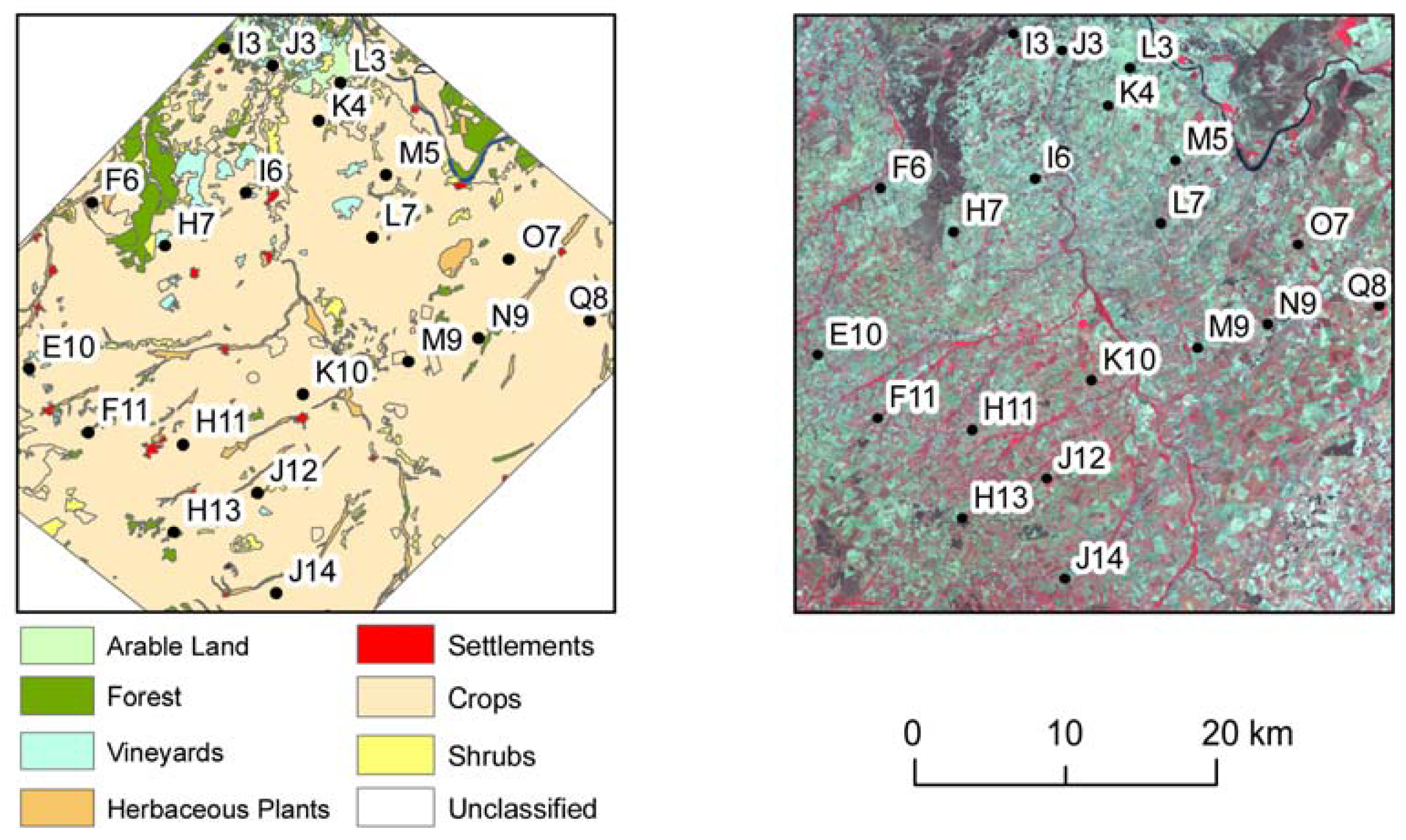
3.1. Test Site

The test site is a region of 4200 km² that surrounds the 1285 km² REMEDHUS network area located in the centre of the Duero basin, Spain, where the University of Salamanca has been operating in-situ soil moisture stations since 1999 (Figure 1) [39].

The area is characterized by a Mediterranean climate with mean annual precipitation of 385 mm and mean annual evapotranspiration of around 908 mm. The geological substrate mainly consists of sandstones, conglomerates and fluvial deposits. The soils within the test site area are dominated by sandy textures. The area is intensively used for farming. The main crops are cereals and grapes. A network of 20 permanent time domain reflectometry (TDR) soil moisture stations is spread over the test site area. At each station two-wire TDR probes (Tektronix 1512C) were installed at 5 cm, 25 cm, 50 cm and 100 cm depths. Only the values taken at 5 cm were used in this study. Comprehensive laboratory analyses of soil samples were carried out to calibrate the TDR measurements and to assess soil properties at each station (texture, porosity, etc.). After the calibration phase, readings have been taken fortnightly since spring 1999. The land cover map and the location of the TDR stations are shown in Figure 1.

The network has repeatedly served for soil moisture process studies [39, 40] and for validating remotely sensed soil moisture data [8, 41]. It will be one of the European validation sites for the Soil Moisture and Ocean Salinity (SMOS) mission [42].

3.2. Satellite Data

Backscatter time series can be obtained from SAR instruments that are capable of acquiring imagery with a high spatial resolution independent of cloud cover and light conditions. However, many spaceborne SAR systems are characterized by short duty cycles (acquisition time per satellite orbit) and small swath width (< 100 km). Therefore, long and dense time series of several dozens or more SAR images covering the same area are generally not available. Coverage can be much improved by increasing the duty cycle and/or by using ScanSAR technology to image a wide swath [43]. The improved coverage however comes at the expense of a lower spatial and radiometric resolution.

For this study, ScanSAR data acquired by the European satellite ENVISAT have been used. ENVISAT was launched on February 28, 2002 by the European Space Agency and circles the earth in a polar 35-days repeat orbit at an altitude of around 800 km and an inclination of 98.5°. The satellite carries the Advanced Synthetic Aperture Radar (ASAR) which is operated at a frequency of 5.331 GHz (C-band). ASAR has two ScanSAR modes which cover a swath of 405 km width [44]. The first ScanSAR mode is the Wide Swath (WS) mode with a spatial resolution of 150 m, a radiometric accuracy of < 0.6 dB and a maximum duty cycle of 30 %. The second one is the Global Monitoring (GM) mode with a spatial resolution of 1 km, a radiometric accuracy of about 1.5 dB and a duty cycle of 100 %. For this investigation, 73 vertically polarised ASAR WS images have been acquired over the REMEDHUS network in the years 2003 to 2006.

4. Methods

4.1. Pre-Processing of ASAR Data

Pre-processing of the ASAR WS data consisted of several steps including georeferencing, radiometric calibration and normalisation. ASAR data require georeferencing with respect to earth curvature and terrain for further processing [45]. The radiometric calibration of SAR images has to involve corrections for the scattering area, the antenna gain pattern and the range spread loss. As the study area shows little topographic variation, the GTOPO30 digital elevation model (improved with SRTM data) proved sufficient for geocoding of the WS data. In the normalisation step the effects on the backscatter due to varying incidence angle and distance from sensor (near and far range) are removed [46]. Because of the limited incidence angle range of ASAR WS images (20-40°), a linear model has proven sufficient to extrapolate backscatter measurements to a reference angle of 30°

$${\sigma }^0(30)={\sigma }^0(\mathit{\vartheta })-\beta (\mathit{\vartheta }-30)$$

(21)

where ϑ is the local incidence angle. Similar to [47] and [48] the slope β was estimated by fitting Equation (21) to all 73 backscatter measurements taken over one location (pixel).

4.2. Analysis of Soil Moisture Scaling Properties

The soil moisture scaling properties of the REMEDHUS network were studied by [49] and [40] by calculating the mean and standard deviation of the relative difference δ_i,j as given by Equation (2). This analysis demonstrated the high degree of persistence of spatial soil moisture patterns within the REMEDHUS network. This suggests that the time-invariant scaling equations as given by (3) and (5) are applicable. To verify this hypothesis, the fit of the time-invariant downscaling Equation (5) is investigated by means of a linear regression analysis between paired data (θ_r, θ_P) extracted from the REMEDHUS data base. To allow a direct comparison with parameters derived from ASAR, all soil moisture values are expressed in degree of saturation, i.e. relative θ_P is computed by dividing volumetric soil moisture values by the total water capacity (which is known for each station). Regional soil moisture θ_r is then estimated by averaging all in-situ soil moisture measurements within the test area according to Equation (1). The accuracy of the downscaling model (5) is described by the coefficient of determination R² and the standard error of the estimate (SEE) which is the standard deviation of the residuals.

4.3. Analysis of Backscatter Scaling Properties

The theoretical discussion in section 2 suggested that within a time period [t−Δt/2, t+Δt/2], local and regional scale backscatter measurements are linearly related according to Equation (16). It is straight forward to validate this prediction from SAR image time series for selected time periods, provided that a sufficient number of images are available for the statistical analysis within these periods. The regional backscatter values were generated by averaging the normalized ASAR backscatter data over a rectangular window of 60 × 70 km². The local scale is 150 m which corresponds to the spatial resolution of ASAR WS mode. By performing a linear regression analysis for each 150 m pixel across the images from the selected time period, the spatial patterns of the model coefficients a and b are obtained. In addition, the uncertainty intervals of a and b, the coefficient of determination R², and the standard error of estimate (SEE) are calculated. To study seasonal vegetation effects, the linear regression was performed for each month based on ASAR data from all years (2003-2006). To make sure that at least 20 images were available for the regression, a relative long time window of Δt = 5 months had to be chosen, i.e. the results for May represent the mean conditions for the period March to July. The effect of this long time window is to suppress changes taking place at daily to weekly time scales, but it should nevertheless be possible to distinguish the main vegetation periods.

At this stage, the parameters describing the fit of the linear backscatter scaling model (16) are known. These empirical results are sufficient for accepting or rejecting the main hypothesis of this study that temporally stable soil moisture patterns lead to temporally stable backscatter patterns. However, it is also of interest to investigate how well the model developed in section 2.2. can predict the backscatter scaling coefficients a and b. As can be seen in equations (17) and (18) six parameters are needed for calculating a and b: the two soil moisture downscaling coefficients, c_lr and d_lr, and the dry backscatter reference value σ⁰_dry and the sensitivity S at local and regional scale respectively. The local scale backscatter model parameters are estimated from the SAR image time series by calculating the mean and standard deviation of σ⁰_l for each 150 m pixel and by setting:

$$S_l=4\cdot \mathit{\text{StDev}}({\sigma }_l^0)$$

(22)

$${\sigma }_{\mathit{\text{dry}},l}^0=\langle {\sigma }_l^0\rangle -2\cdot \mathit{\text{StDev}}({\sigma }_l^0)$$

(23)

where the brackets indicate the mean. If σ⁰_l is normally distributed, about 95 % of all values are within the interval defined by the dry backscatter reference value σ⁰_dry and the sensitivity S_l. Even though this definition is somewhat arbitrary it was preferred over selecting individual images as dry respectively wet reference values because it was not possible to identify ASAR acquisitions where the entire area was dry respectively wet. The regional scale backscatter parameters are obtained by simply averaging S_l and σ⁰_dry,l over the entire study area. While estimates of S_l and σ⁰_dry,l are now available for the entire study area, the detailed spatial patterns of c_lr and d_lr are not known. However, on average, c_lr must be equal to zero and d_lr equal to one if relative soil moisture averages linearly. Therefore, the following model represents a first approximation to the coefficients a and b:

$$a(x,y,\overline{t})\approx {\sigma }_{\mathit{\text{dry}},l}^0(x,y,\overline{t})-\frac{S_l(x,y,\overline{t})}{S_r(\overline{t})}{\sigma }_{\mathit{\text{dry}},r}^0(\overline{t})$$

(24)

$$b(x,y,\overline{t})\approx \frac{S_l(x,y,\overline{t})}{S_r(\overline{t})}$$

(25)

The modelled parameters were then compared to the observed values of a and b. The accuracy of the prediction is assessed by the coefficient of determination R² and the root mean square error (RMSE).

4.4. Estimation of Soil Moisture Scaling Properties from ASAR

The soil moisture scaling parameters c_lr and d_lr are calculated according to equations (19) and (20) based on the ASAR image time series. The retrieved maps of c_lr and d_lr are assessed using the land cover information available for the REMEDHUS area. Also, c_lr and d_lr are compared to c_pr and d_pr derived from the in-situ measurements despite the apparent mismatch of spatial scales.

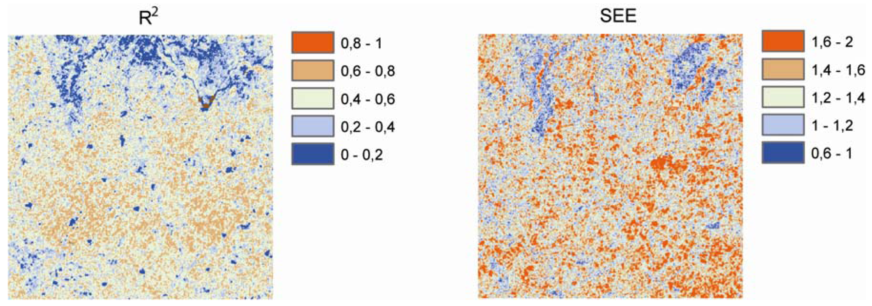
5. Results and Discussion

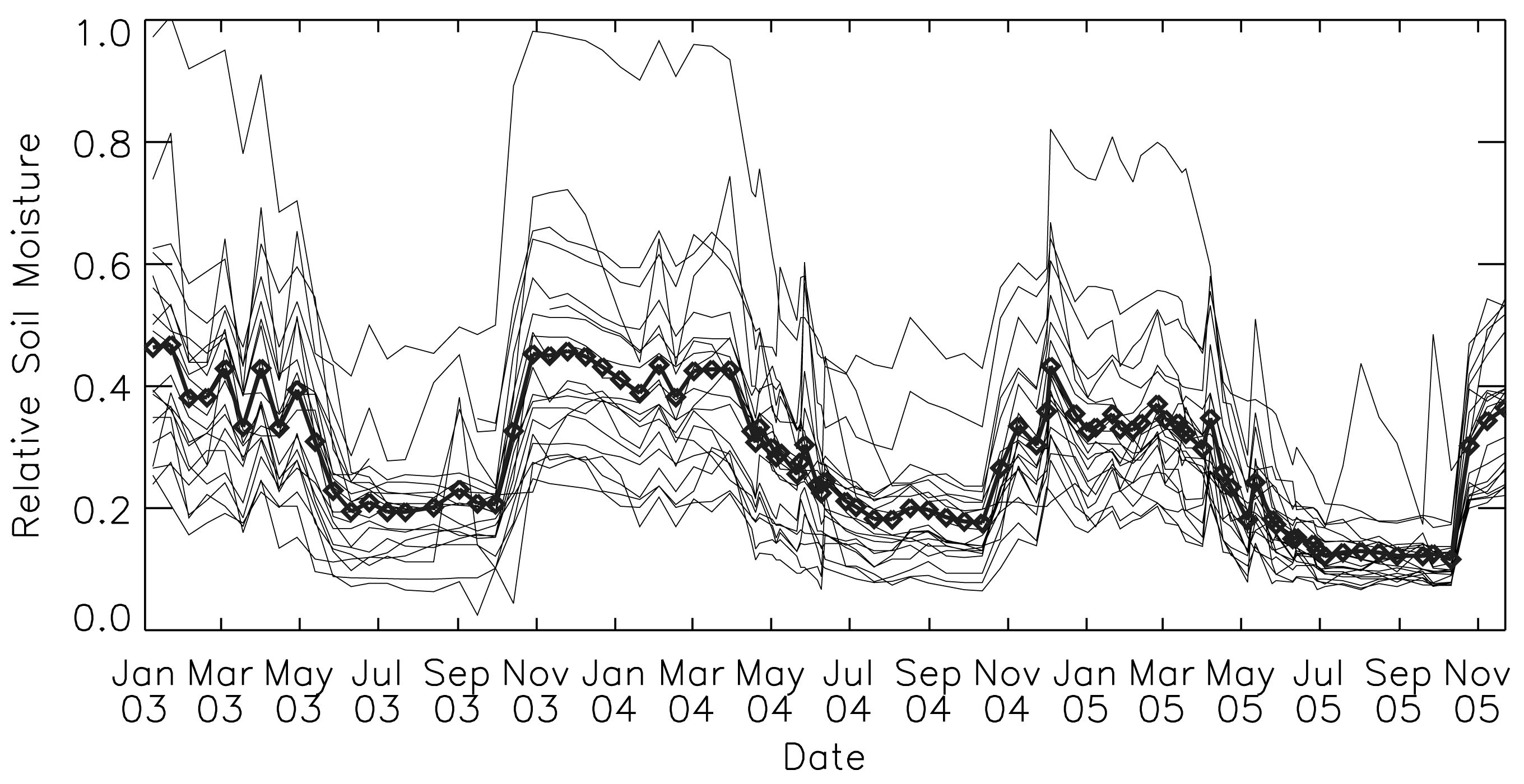
5.1. Soil moisture scaling properties from in-situ measurements

Soil moisture data from the 20 soil probes installed at 5 cm of the REMEDHUS network are plotted in time together with the spatial mean in Figure 2. It can be seen that the temporal variation of the soil moisture values at individual stations to a large extent follows that of the mean soil moisture. However, the absolute values and dynamic ranges differ from station to station. These observations are confirmed by Figure 3 which shows scatter plots of point scale soil moisture, θ_p, versus regional scale soil moisture, θ_r, for three selected stations of the REMEDHUS network. One can see that a linear downscaling model as given by Equation (5) is quite appropriate for describing the soil moisture scaling properties. The results for all TDR stations are summarized in

Table 1. Soil scaling parameters computed from the relative soil moisture data collected at 20 stations of the REMEDHUS network: soil composition, mean relative difference δ_i,j, standard deviation from the mean relative difference Stdev (δ_i,j), soil moisture downscaling coefficients c_pr and d_pr, coefficient of determination (R²), and standard error of the estimate (SEE).

				In-situ						ASAR
Station	Sand (%)	Silt (%)	Clay (%)	δi,j [%]	Stdev (δi,j)	cpr	dpr	R2	SEE	clr	dlr
E10	75.1	16.4	8.5	-47.50	9.26	-0.04	1.43	0.69	0.09	0.03	0.93
F6	67.2	13.7	19.1	-32.60	18.32	0.02	2.03	0.79	0.10	0.01	0.97
F11	81.5	12.0	6.5	-29.89	18.13	-0.04	0.93	0.89	0.03	-0.02	1.03
H7	85.1	9.6	5.3	-27.76	26.17	0.10	0.34	0.49	0.03	0.02	0.96
H11	79.7	10.2	10.1	-27.13	27.17	0.03	1.26	0.75	0.07	-0.02	1.04
H13	70.4	11.5	18.2	-22.98	14.88	0.02	0.77	0.69	0.05	-0.08	1.16
I3	90.2	6.3	3.5	-18.28	15.37	0.01	1.08	0.78	0.05	-0.02	1.04
I6	89.8	5.9	4.3	-16.38	37.73	0.06	0.85	0.73	0.05	0.08	0.83
J3	85.1	11.3	3.7	-16.27	20.45	0.00	0.73	0.57	0.06	0.02	0.96
J12	60.9	16.9	22.2	-14.99	20.66	0.03	1.38	0.85	0.05	0.02	0.97
J14	66.8	21.0	12.2	-12.12	23.17	-0.02	0.90	0.84	0.04	-0.09	1.18
K4	87.1	9.3	3.6	-8.48	19.47	0.02	0.61	0.65	0.04	-0.03	1.05
K10	91.2	5.7	3.1	5.54	22.37	-0.04	0.86	0.77	0.04	-0.06	1.13
L3	82.3	6.4	11.3	9.85	25.04	0.03	0.80	0.77	0.04	0.02	0.95
L7	46.8	20.8	32.4	14.79	12.17	-0.03	0.94	0.49	0.09	-0.06	1.13
M5	81.6	8.3	10.1	18.02	16.12	0.00	1.17	0.89	0.04	0.06	0.88
M9	49.8	24.9	25.3	29.04	39.59	0.01	1.10	0.92	0.03	-0.07	1.15
N9	62.5	16.8	20.8	38.26	43.75	-0.07	1.09	0.82	0.05	-0.05	1.10
O7	78.8	13.5	7.7	48.70	25.93	0.00	0.51	0.84	0.02	0.00	1.01
Q8	86.1	5.7	8.3	110.78	46.90	-0.10	1.22	0.81	0.06	0.28	0.44
Mean	75.9	12.3	11.8	0.03	24.13	0.00	1.00	0.75	0.05	0.00	1.00
Stdev	13.1	5.6	8.4	36.41	10.40	0.05	0.37	0.12	0.02	0.08	0.16

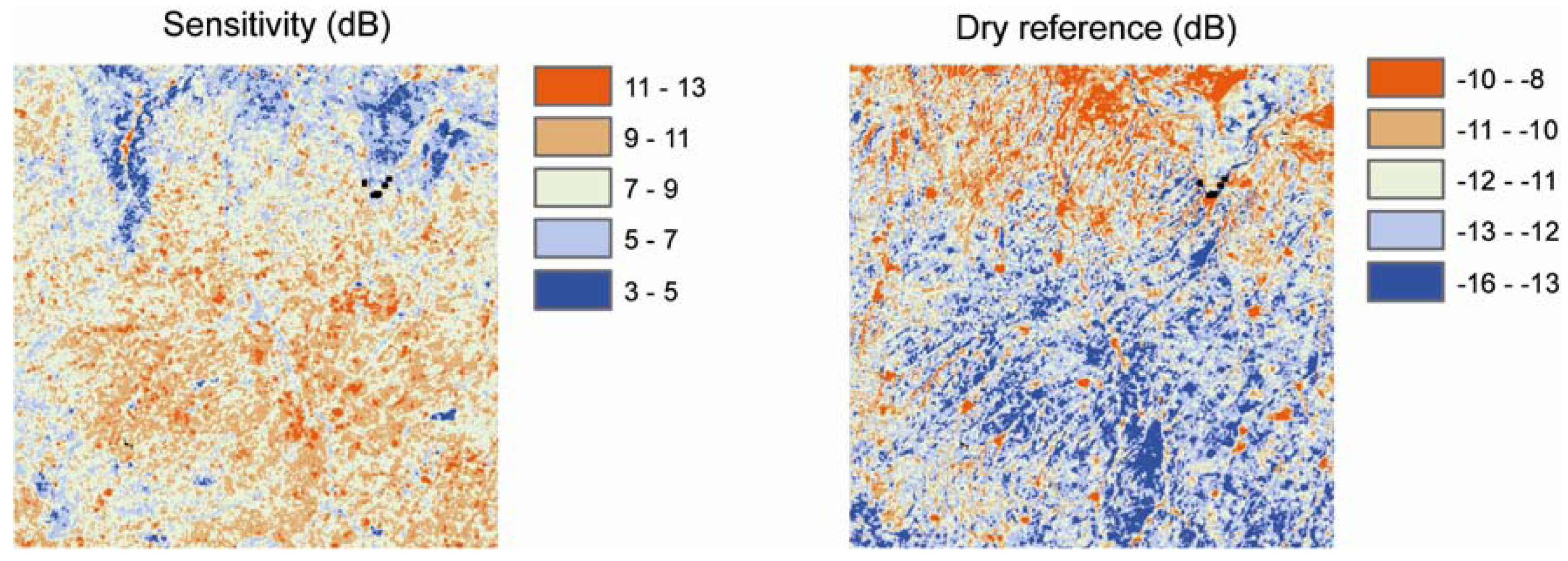
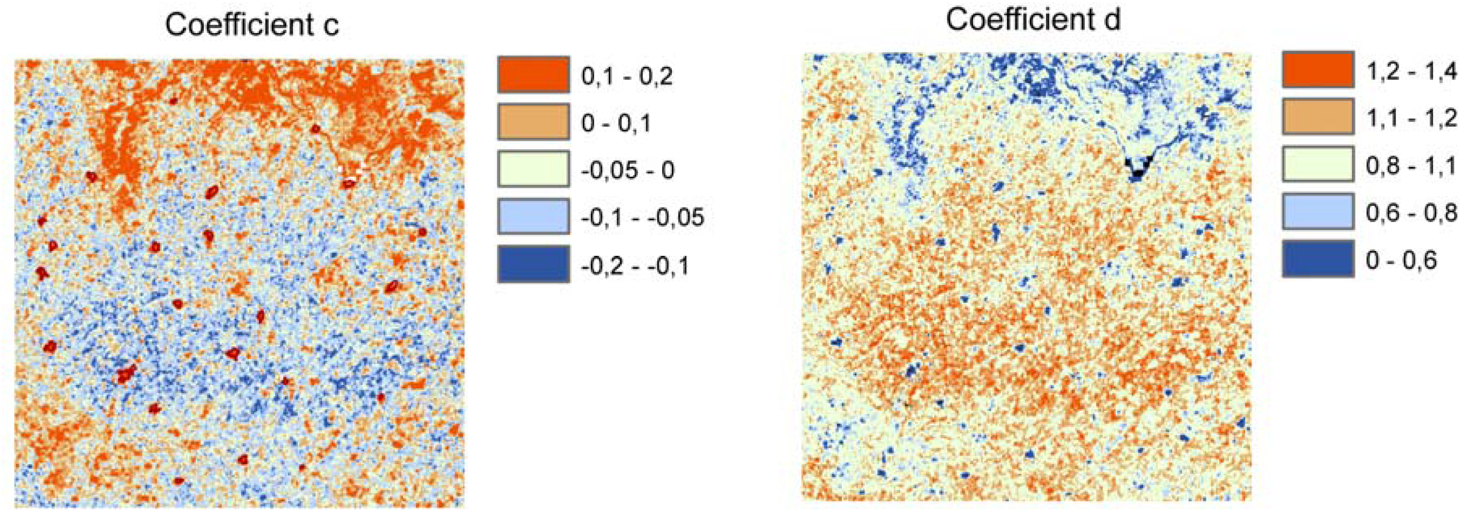
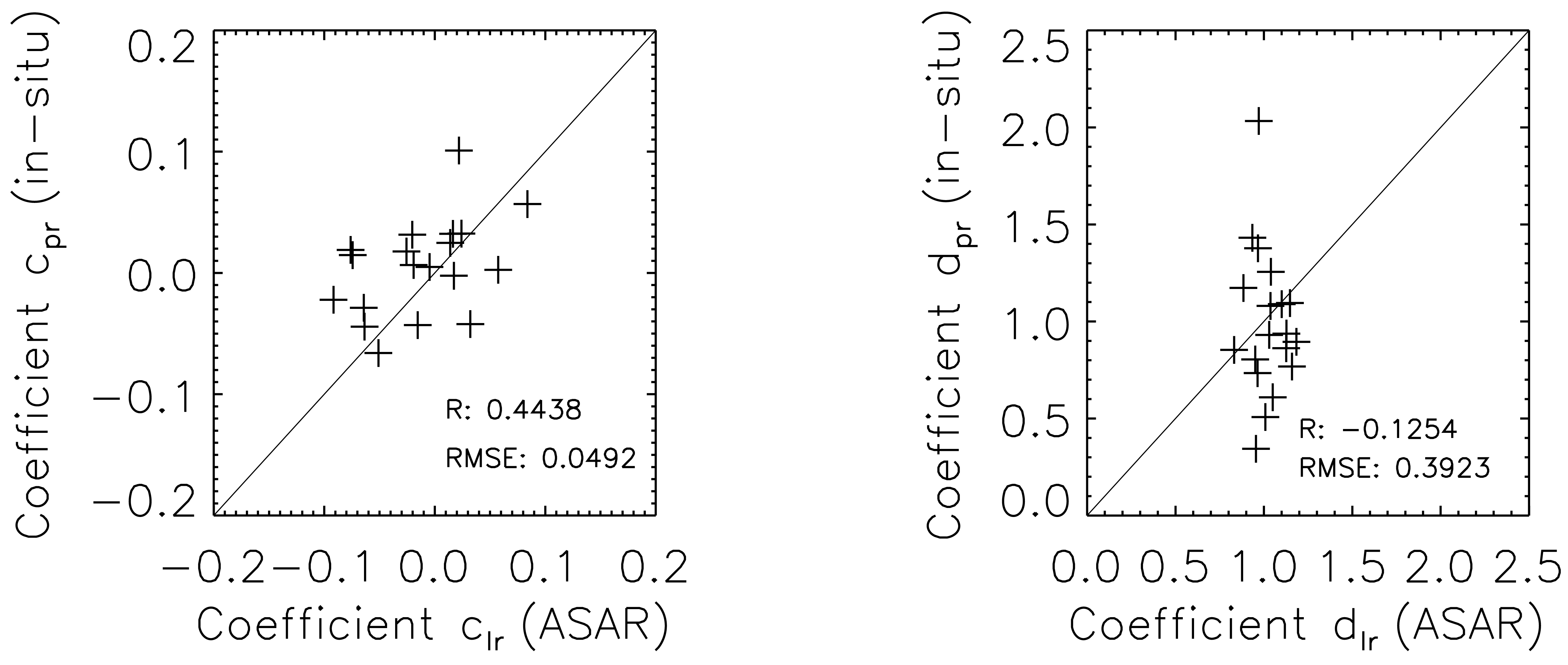
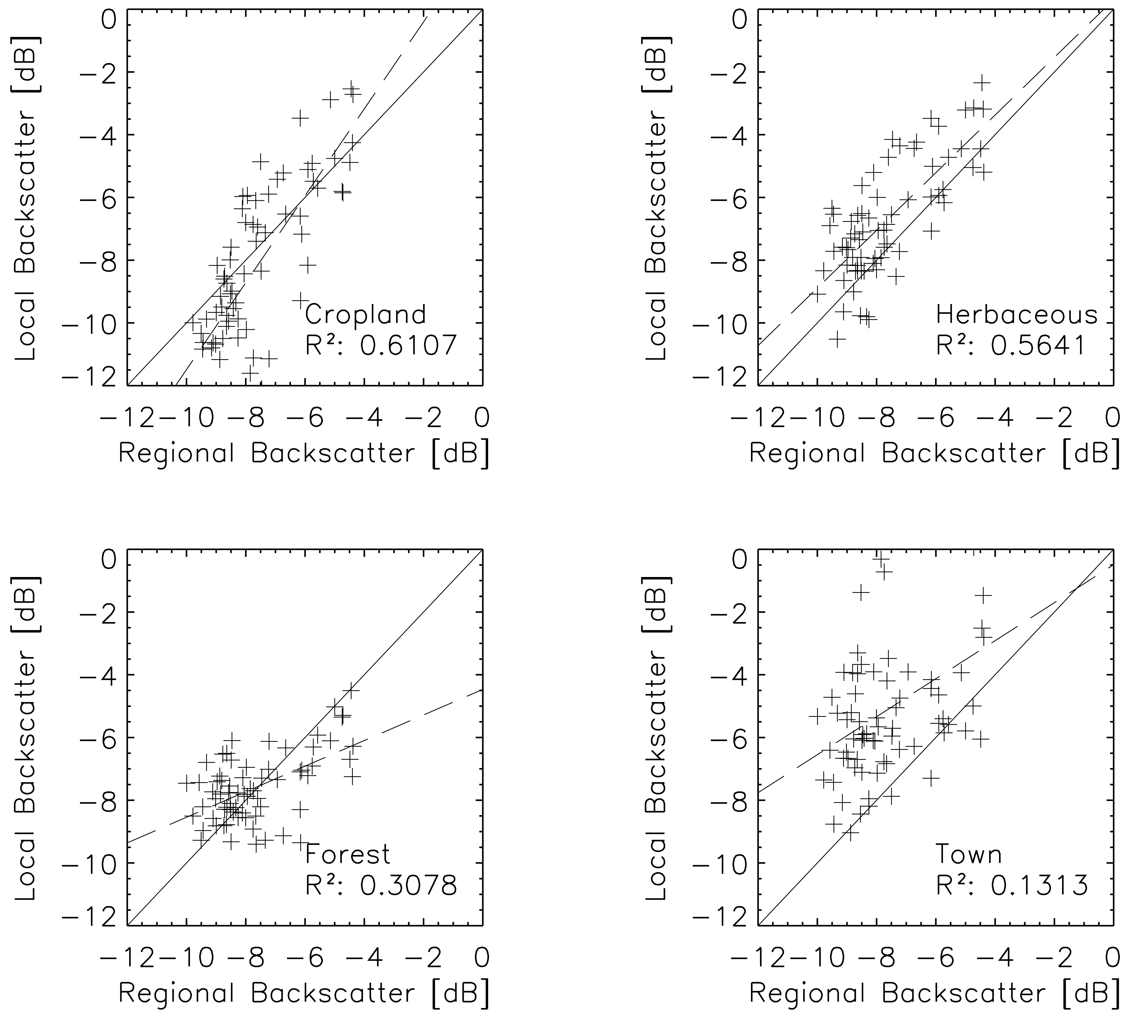
. It is found that the coefficient of determination is in general relatively high with a mean value of 0.75. The standard error of estimate is on average only 5 % relative soil moisture. Therefore it can be concluded that the linear downscaling model (5) is well suited for connecting the point scale to the regional scale $ℛ$. By mathematical deduction it is also possible to confirm the suitability of Equation (13) to connect the local ($ℒ$) and regional ($ℛ$) scale (section 2.2.).

Table 1 also shows that both downscaling coefficients vary over a relatively large range (c_pr from −0.1 to 0.1 and d_pr from 0.34 to 2.03). In particular, the large variability of d_pr implies that the results are not easily comparable to the parameters of the classical temporal stability analysis as proposed by [7], because the latter only considers the mean and standard deviation of the relative difference (also shown in Table 1). Overall, the results are well in line with findings of other authors [13, 14, 18, 19].

5.2. Backscatter scaling properties observed by ASAR

A first impression about the relationship between local and regional backscatter can be obtained from scatter plots such as shown in Figure 4. All 73 ASAR images were used to create these plots. Instrument noise, radar speckle, inaccuracies in the incidence normalisation, agricultural farming practices and seasonal vegetation effects all add to an increasing spread of the point cloud. Nevertheless, one can see that there is a comparably strong correlation between σ⁰_l and σ⁰_r for areas covered by low vegetation, which progressively becomes weaker with increasing vegetation biomass. Over urban areas backscatter is high and relatively stable. This is in agreement with equations (16) and (18) which show that the relationship between σ⁰_l and σ⁰_r is primarily controlled by the local sensitivity of σ⁰ to soil moisture.

Because of the important role of S_l for explaining the backscatter scaling properties for different land cover classes, it is expected that a and b vary seasonally depending on vegetation status. However, a comparison of a and b values computed for all months with a 5-months moving window does not reveal a clear seasonal pattern. As Figure 5 shows for two representative sites, the temporal variability of a and b lies within the limits of their uncertainty. One explanation is that it is the ratio of local and regional scale sensitivity S_l/S_r, which enters equations (17) and (18), and not the local sensitive S_l alone. Also, seasonal changes in the dry backscatter reference do not appear to be important because a is related to the difference of local scale and regional scale σ⁰_dry. Another explanation is that in the incidence angle range from 20 to 40°, the effects of vegetation phenology on the C-band backscatter measurements is in general much weaker than the soil moisture signal. A previous analysis of ERS scatterometer measurements over the REMEDHUS network has shown that the sensitivity of backscatter to soil moisture at an incidence angle of 40° is approximately 5 dB in summer and 6 dB in winter, i.e. vegetation contributes only 1 dB to the total temporal signal at regional scale [41].

Because of this absence of seasonal effects in a and b, Equation (16) can be written as:

$${\sigma }_l^0(x,y,t)=a(x,y)+b(x,y){\sigma }_r^0(t)$$

(26)

All further calculations will therefore be based on all available ASAR WS images.

Spatial images of the coefficient of determination (R²) and the standard error of estimate (SEE) of the linear backscatter scaling model (16) are shown in Figure 6. As expected, R² in general is high over agricultural areas and other sparsely vegetated terrain with values up to about 0.8. The correlation decreases with increasing vegetation density and becomes smaller than 0.2 over dense forests and urban areas. The standard error of estimate shows very similar spatial patterns. Over areas characterised by relatively stable backscatter (and hence low R²) SEE may be as low as 0.6 dB which corresponds to the noise of the ASAR Wide Swath measurements. With decreasing vegetation density SEE increases. One important reason for this is that over bare or sparsely vegetated terrain, backscatter shows a pronounced incidence angle dependency. Therefore, uncertainties related to the normalisation Equation (21) have a stronger effect on the accuracy of σ⁰(30) over these areas compared to more densely vegetated areas. Also, agricultural activities such as ploughing or harvesting may cause outliers. Nevertheless, SEE does not exceed 2 dB even over agricultural fields characterised by a steep σ⁰(ϑ) curve. Therefore, it is concluded that the linear time-invariant backscatter model (26) is well suited for describing the spatio-temporal behaviour of radar backscatter across different spatial scales. This also corroborates the finding from the analysis of the in-situ measurements that spatial soil moisture patterns in general exhibit a high degree of temporal persistence.

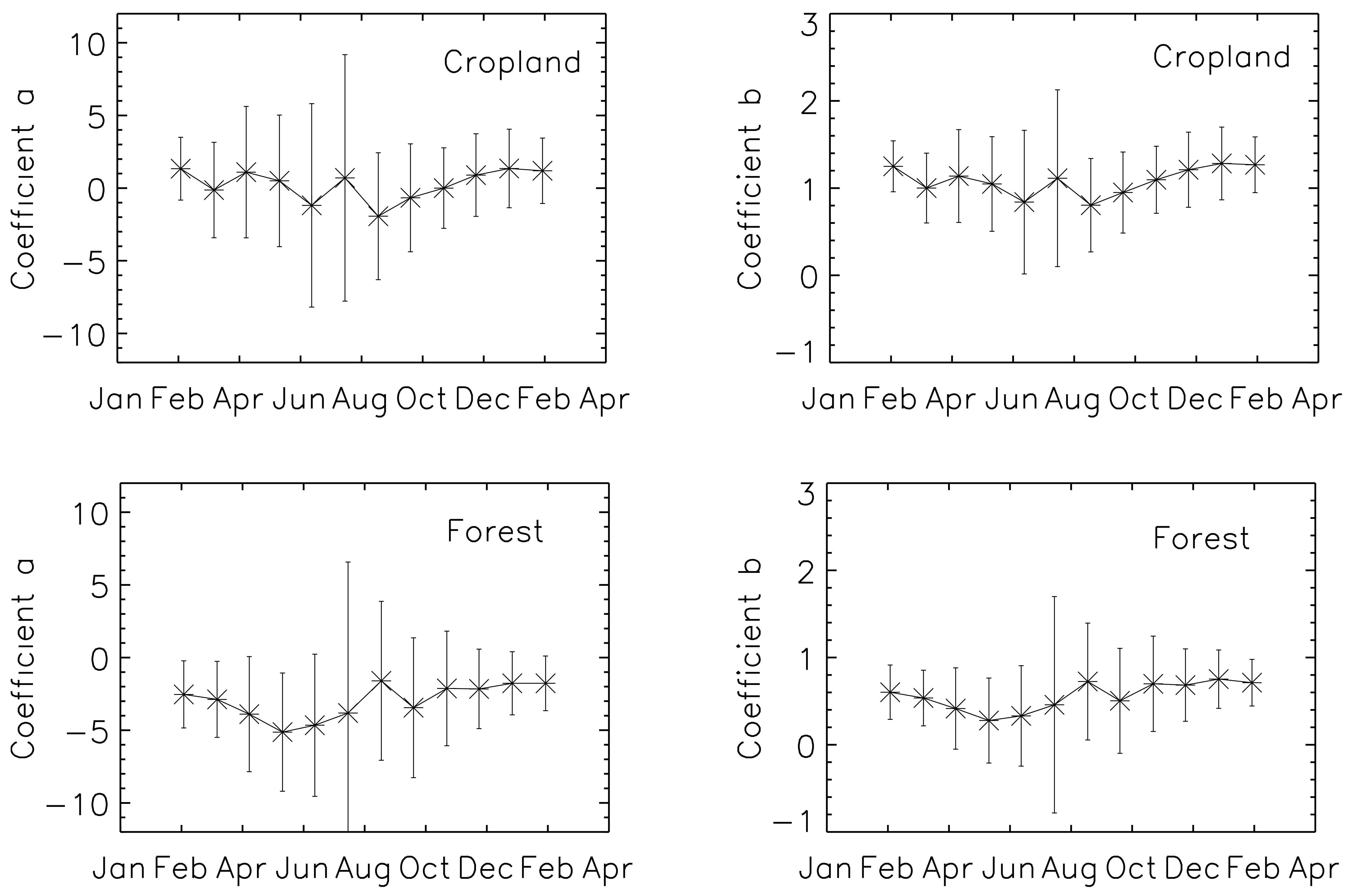
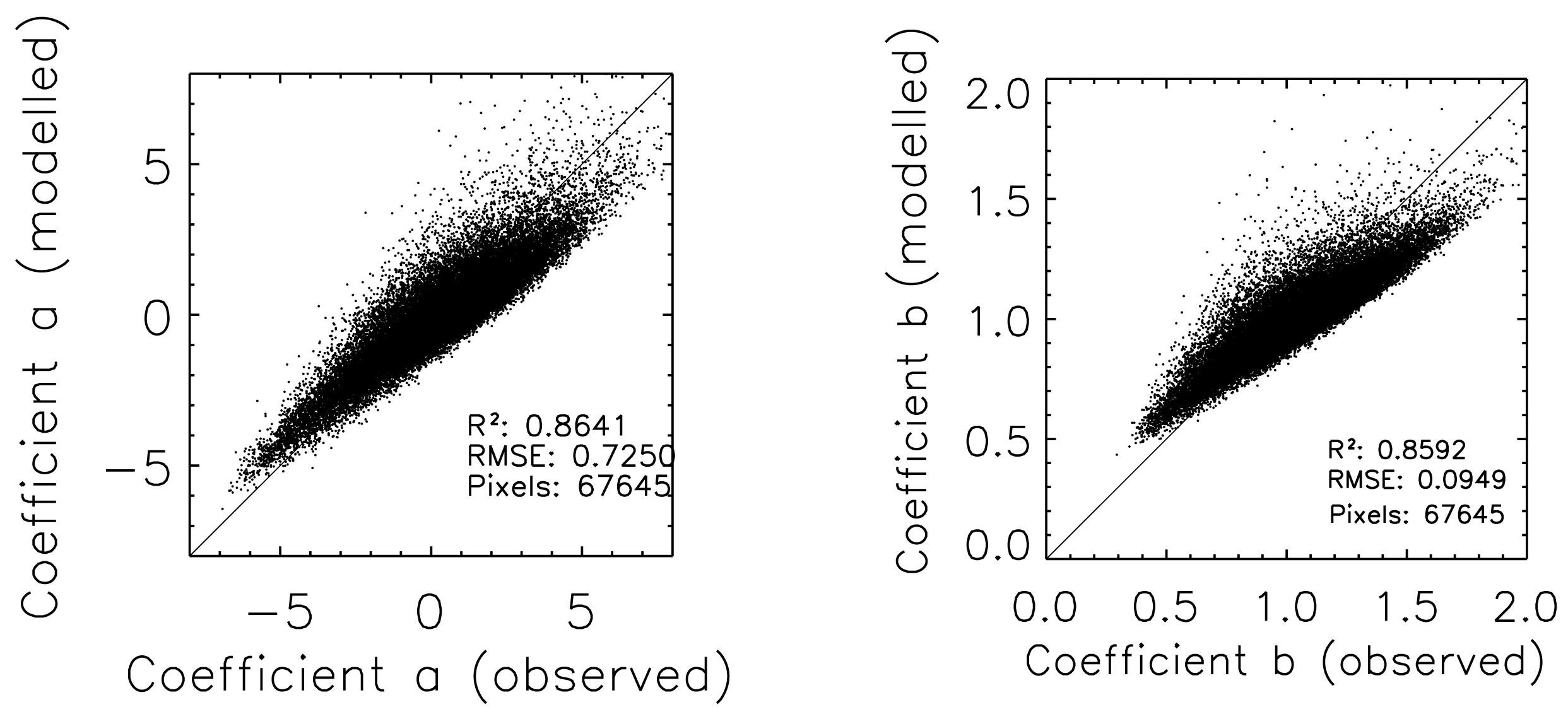
5.3. Backscatter scaling coefficients

As expected, the backscatter scaling parameters a and b derived from the ASAR WS images show a pronounced spatial pattern (Figure 7 left). Forests, shrubs and more dense herbaceous plants in the vicinity of small streams can be distinguished from cropland. Settlements show a similar behaviour as dense vegetation. To check the validity of the backscatter scaling model as developed in section 2.2., the sensitivity and dry backscatter reference were calculated according to equations (22) and (23) based on all 73 ASAR images. The assumption is that also S and σ⁰_dry can in a first approximation be treated as constants at both scales. Equations (24) and (25) thus simplify to

$$a(x,y)\approx {\sigma }_{\mathit{\text{dry}},l}^0(x,y)-\frac{S_l(x,y)}{S_r}{\sigma }_{\mathit{\text{dry}},r}^0$$

(27)

$$b(x,y)\approx \frac{S_l(x,y)}{S_r}$$

(28)

Figure 8 shows that the sensitivity ranges from about 3 dB for forests and settlements to values exceeding 12 dB for some agricultural fields. Disregarding settlements, the spatial pattern of S_l thus conveys a good impression of the spatial distribution of vegetation in the study area. Despite being more strongly influenced by surface roughness, also the dry backscatter reference reflects vegetation patterns well, with values ranging from −16 dB for agricultural fields up to -8 dB for forests and settlements. Based on these two parameters, the backscatter scaling coefficients a and b can be calculated according to models (26) and (27). The modelled values are compared to the observed ones in Figure 7. One can see that the spatial patterns of both scaling coefficients are very well reproduced by this model, although the dynamic range of the modelled a and b images is somewhat smaller.

This can be more clearly observed in Figure 9 which shows scatter plots between observed and modelled coefficients. The smaller dynamic range is likely related to the fact that c_lr was set equal to zero and d_lr equal to one in order to obtain the simplified models (24) and (25). Nevertheless, the high correlation between the observed and modelled coefficients (R² = 0.86 for both a and b based on 67645 data points) and the low root mean square error (0.73 dB for a and 0.095 for b, which corresponds to a relative error of about 5 % in both cases) clearly show that the backscatter scaling model developed in section 2.2. describes the main physical phenomena very well.

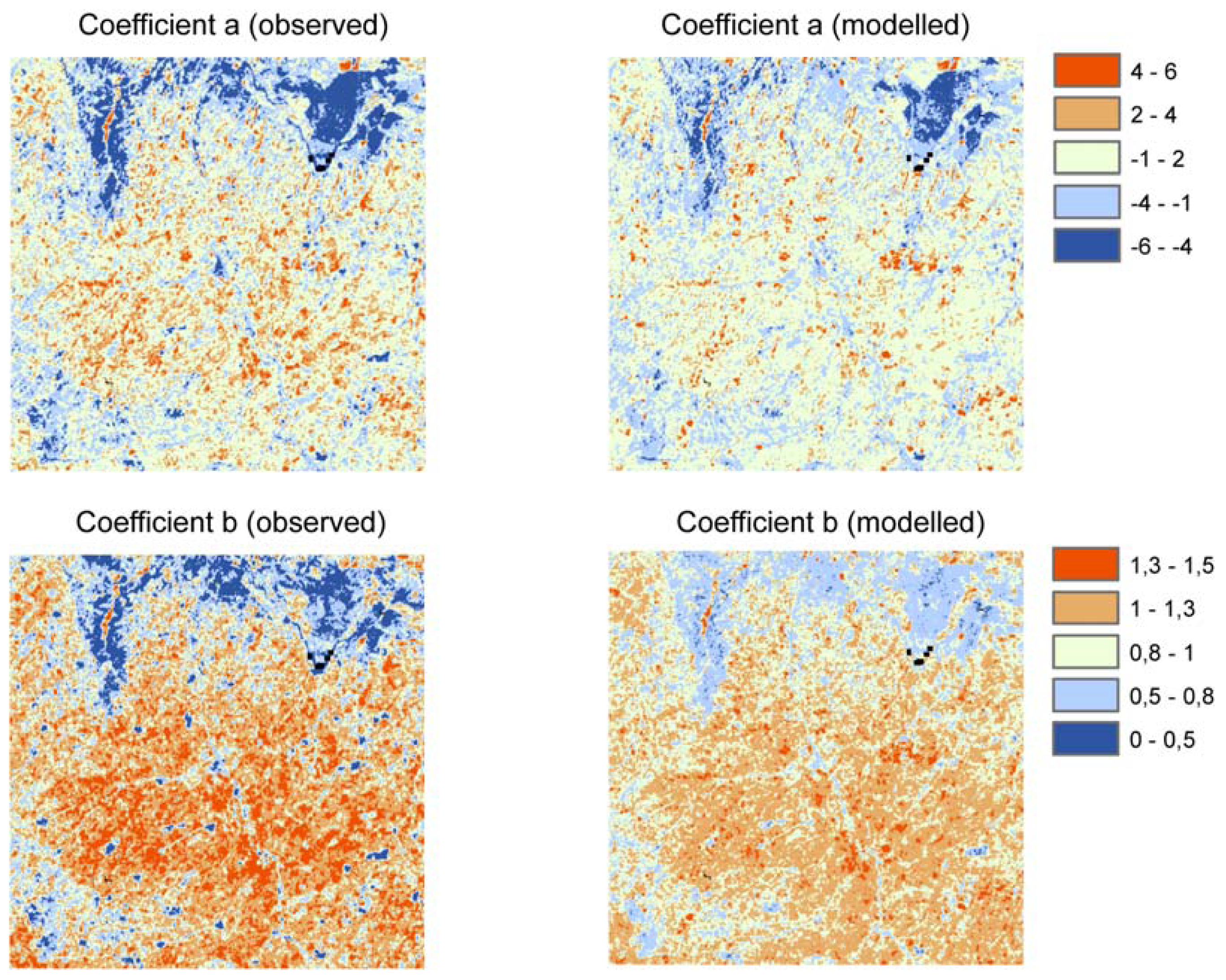
5.4. Soil moisture scaling parameters derived from ASAR

Having confirmed the validity of the backscatter scaling model, equations (19) and (20) can be used to estimate the soil moisture scaling coefficients c_lr and d_lr from the ASAR WS image time series. Again, all parameters of the equations are assumed to be constant in time:

$$c_{\mathit{\text{lr}}}(x,y)=\frac{a(x,y)+b(x,y){\sigma }_{\mathit{\text{dry}},r}^0-{\sigma }_{\mathit{\text{dry}},l}^0(x,y)}{S_l(x,y)}$$

(29)

$$d_{\mathit{\text{lr}}}(x,y)=b(x,y)\frac{S_r}{S_l(x,y)}$$

(30)

The retrieved maps of c_lr and d_lr are shown in Figure 10. One can see that c_lr tends to be positive for forests and settlements and predominantly negative over the agricultural areas. Similar but inverted patterns are observed in d_lr which takes on values below one for dense vegetation and settlements and values above one for agricultural land. These results suggests that in forests and more dense vegetation, surface soil moisture conditions are less variable compared to the surrounding agricultural land. Within the agricultural area, c_lr and d_lr show comparably little spatial variation, with the exception of some agricultural fields. These outliers may be related to irrigation, which is applied in the study area and cause c_lr to reach higher and d_lr to reach lower values comparable to non-irrigated fields. An example of the irrigation effect on coefficients c_lr and d_lr is observed at the ASAR pixel closest to the REMEDHUS station Q8 (Table 1). Thus, this measurement was excluded from further statistical comparisons. Equally, it is not unlikely that irrigation is responsible for the behaviour of c_lr and d_lr in and near settlements.

Finally, the ASAR derived backscatter scaling coefficients are compared to the ones derived from the in-situ measurements. Due to the scale mismatch (0.1 to 10 dm² for the in-situ measurements versus 2.25 ha for the ASAR WS pixels) and the differences in size and orientation of the ASAR pixel and the agricultural fields makes the comparison problematic. In fact, there is no correlation between d_pr from the in-situ measurements and d_lr from ASAR. One can see from Figure 11 that d_pr is characterised by much larger dynamic range compared to d_lr which is expected when going from point to local scale. Nevertheless, Figure 11 (left) also shows that there is weak but statistical significant relationship between c_pr from the in-situ measurements and c_lr from ASAR (R = 0.44 and RMSE = 0.0492).

6. Conclusions

The spatio-temporal distribution of soil moisture is the result of highly non-linear atmospheric and hydrological processes. Similarly, backscatter observed by radar instruments is a complex function of vegetation and soil parameters. Yet, quite regular spatio-temporal patterns emerge out of these nonlinear processes. This study demonstrates that temporally stable soil moisture patterns lead to temporally stable radar backscatter patterns. This means that time-invariant relationships can be used for connecting soil moisture and radar backscatter measurements across different spatial scales. The analysis of in-situ soil moisture measurements and ASAR image time series acquired over the REMEDHUS network located in the Duero basin, Spain, showed that simple linear time-invariant models can be used to predict soil moisture and radar backscatter at point and local scales based on regional observations, and vice versa.

To gain a better understanding of the underlying physical phenomena, a model was developed to explain the magnitude of the observed backscatter scaling coefficients a and b based on the scattering properties of the terrain and vegetation. A comparison of observed and modelled coefficients yielded a high correlation (R² = 0.86) and a low relative error of 5 % for both parameters respectively. This suggests that the model captures the main physical effects well. The model was subsequently used to estimate soil moisture scaling parameters c_lr and d_lr from the ASAR data. The results are plausible in that the spatial variations in the ASAR derived scaling coefficients can be explained by vegetation. Also, the comparison of c_lr and d_lr with the respective scaling parameters c_pr and d_pr derived from the in-situ observations showed a weak but significant correlation between c_lr and c_pr. However, more in-situ observations are required for a more quantitative comparison of the scaling coefficients obtained by the two methods, in particular from forests.

An important application of the methods developed in this study lies in the interpretation of coarse resolution soil moisture data derived from METOP ASCAT at sub-pixel level. By analysing long ENVISAT ASAR image time series it is possible to identify those sub-pixel areas that contribute to the soil moisture signal observed by ASCAT. Furthermore, ASAR retrieved scaling coefficients may be used for downscaling ASCAT soil moisture data. Because active and passive microwave measurements deal, in principle, with the same physical phenomena [50], these methods should also be of relevance for passive microwave instruments such as AMSR-E and SMOS.

References and Notes

1. Western, A. W.; Blöschl, G. On the spatial scaling of soil moisture. Journal of Hydrology. 1999, 217, 203–224. [Google Scholar]
2. Dubayah, R.; Wood, E. F.; Lavallée, D. Multiscaling Analysis in Distributed Modelling and Remote Sensing: An Application Using Soil Moisture. In Scale in Remote Sensing and GIS; Quattrochi, D. A., Goodchild, M. F., Eds.; Boca Raton, Boston, London, New York, Washington, D.C.; Lewis Publishers, 1997. [Google Scholar]
3. Raju, S.; Chanzy, A.; Wigneron, J.; Calvet, J.; Kerr, Y.; Laguerre, L. Soil moisture and temperature profile effects on microwave emission at low frequencies. Rem. Sens. Environ. 1995, 54, 85–97. [Google Scholar]
4. Entin, J. K.; Robock, A.; Vinnikov, K. Y.; Hollinger, S. E.; Liu, S.; Namkhai, A. Temporal and spatial scales of observed soil moisture variations in the extratropics. Journal of Geophysical Research. 2000, 105(D9), 11865–11877. [Google Scholar]
5. Western, A. W.; Zhou, S.-L.; Grayson, R. B.; McMahon, T. A.; Blöschl, G.; Wilson, D. J. Spatial correlation of soil moisture in small catchments and its relationship to dominant spatial hydrological processes. Journal of Hydrology 2004, 286(1-4), 113–134. [Google Scholar]
6. Vinnikov, K. Y.; Robock, A.; Speranskaya, N. A.; Schlosser, C. A. Scales of temporal and spatial variability of mitlatitude soil moisture. J. Geophys. Res. 1996, 101(D3), 7163–7174. [Google Scholar]
7. Vachaud, G.; Passerat de Silans, A.; Balabanis, P.; Vauclin, M. Temporal Stability of Spatially Measured Soil Water Probability Density Function. Soil Sci. Soc. Am. J. 1985, 49, 822–828. [Google Scholar]
8. Wagner, W.; Naeimi, V.; Scipal, K.; de Jeu, R.; Martinez-Fernandez, J. Soil moisture from operational meteorological satellites. Hydrogeology Journal. 2007, 15(1), 121–131. [Google Scholar]
9. Njoku, E. G.; Jackson, T. J.; Lakshmi, V.; Chan, T. K.; Nghiem, S. V. Soil moisture retrieval from AMSR-E. IEEE Transactions on Geoscience and Remote Sensing. 2003, 41(2), 215–229. [Google Scholar]
10. Bartalis, Z.; Wagner, W.; Naeimi, V.; Hasenauer, S.; Scipal, K.; Bonekamp, H.; Figa, J.; Anderson, C. Initial soil moisture retrievals from the METOP-A Advanced Scatterometer (ASCAT). Geophysical Research Letters. 2007, 34, L20401. [Google Scholar]
11. Kerr, Y. H. Soil moisture from space: Where are we? Hydrogeology Journal. 2007, 15(1), 117–120. [Google Scholar]
12. Wagner, W.; Blöschl, G.; Pampaloni, P.; Calvet, J.-C.; Bizzarri, B.; Wigneron, J.-P.; Kerr, Y. Operational readiness of microwave remote sensing of soil moisture for hydrologic applications. Nordic Hydrology. 2007, 38(1), 1–20. [Google Scholar]
13. Cosh, M. H.; Jackson, T. J.; Starks, P.; Heathman, G. Temporal stability of surface soil moisture in the Little Washita River watershed and its applications in satellite soil moisture product validation. Journal of Hydrology. 2006, 323, 168–177. [Google Scholar]
14. Grayson, R.; Western, A. W. Towards areal estimation of soil water content from point measurements: time and space stability of mean response. Journal of Hydrology. 1998, 207, 68–82. [Google Scholar]
15. Walker, J. P.; Willgoose, G. R.; Kalma, J. D. In situ measurement of soil moisture: a comparison of techniques. Journal of Hydrology. 2004, 293(1-4), 85–99. [Google Scholar]
16. Cosh, M. H.; Jackson, T. J.; Bindlish, R.; Prueger, J. H. Watershed scale temporal and spatial stability of soil moisture and its role in validating satellite estimates. Remote Sensing of Environment. 2004, 92(4), 427–435. [Google Scholar]
17. Chen, D.; Engman, E. T.; Brutsaert, W. Spatial distribution and pattern persistence of surface soil moisture and temperature over prairie from remote sensing. Remote Sensing of Environment. 1997, 61, 347–360. [Google Scholar]
18. De Lannoy, G. J. M.; Houser, P. R.; Verhoest, N. E. C.; Pauwels, V. R. N.; Gish, T. J. Upscaling of point scale measurements to field averages at the OPE3 test site. Journal of Hydrology. 2007, 343(1-2), 1–11. [Google Scholar]
19. Baup, F.; Mougin, E.; de Rosnay, P.; Timouk, F.; Chênere, I. Surface soil moisture estimation over the AMMA Sahelian site in Mali using ENVISAT/ASAR data. Rem. Sens. Environ. 2007, 109, 473–481. [Google Scholar]
20. Loew, A.; Mauser, W. On the dissagregation of passive microwave data using priori knowledge on temporal persistent soil moisture fields. IEEE Transactions on Geoscience and Remote Sensing. 2008, in press. [Google Scholar]
21. Ulaby, F. T.; Moore, R. K.; Fung, A. K. Microwave Remote Sensing: Active and Passive. Volume 2: Radar Remote Sensing and Surface Scattering and Emission Theory; Addison-Wesley Advanced Book Program: Reading, Massachusetts, 1982; p. 609. [Google Scholar]
22. Fung, A. K. Microwave scattering and emission models and their applications.; Artech House: Boston, 1994. [Google Scholar]
23. Ulaby, F. T.; Sarabandi, K.; McDonald, K.; Whitt, M.; Dobson, M. C. Michigan Microwave Canopy Scattering Model (MIMICS). International Journal of Remote Sensing. 1990, 11(7), 1223–1253. [Google Scholar]
24. Baghdadi, N.; Zribi, M. Evaluation of radar backscatter models IEM, OH and DUBOIS using experimental observations. International Journal of Remote Sensing. 2006, 27(18-20), 3831–3852. [Google Scholar]
25. Walker, J.; Houser, P.; Willgoose, G. Active microwave remote sensing for soil moisture measurement: a field evaluation using ERS-2. Hydrological Processes. 2004, 18(11), 1975–1997. [Google Scholar]
26. Davidson, M.; Le Toan, T.; Mattia, F.; Satalino, G.; Manninen, T.; Borgeaud, M. On the characterisation of agricultural soil roughness for radar remote sensing studies. IEEE Transactions on Geoscience and Remote Sensing. 2000, 38(2), 630–640. [Google Scholar]
27. Moran, M. S.; Hymer, D. C.; Qi, J.; Sano, E. E. Soil moisture evaluation using multi-temporal synthetic aperture radar (SAR) in semiarid rangeland. Agricultural and Forest Meteorology. 2000, 105, 69–80. [Google Scholar]
28. Engman, E. T. Soil moisture. In Remote Sensing in Hydrology and Water Management; Schultz, G. A., Engman, E. T., Eds.; Berlin; Springer, 2000; pp. 197–216. [Google Scholar]
29. Wagner, W.; Lemoine, G.; Borgeaud, M.; Rott, H. A Study of Vegetation Cover Effects on ERS Scatterometer Data. IEEE Transactions on Geoscience and Remote Sensing. 1999, 37(2), 938–948. [Google Scholar]
30. Hillel, D. Introduction to Soil Physics; Academic Press: San Diego, 1982. [Google Scholar]
31. Wagner, W.; Scipal, K.; Pathe, C.; Gerten, D.; Lucht, W.; Rudolf, B. Evaluation of the agreement between the first global remotely sensed soil moisture data with model and precipitation data. Journal of Geophysical Research D: Atmospheres. 2003, 108(D19). Art. No. 4611. [Google Scholar]
32. Pellarin, T.; Calvet, J.-C.; Wagner, W. Evaluation of ERS scatterometer soil moisture products over a half-degree region in southwestern France. Geophysical Research Letters. 2006, 33(17). Art. No. L17401. [Google Scholar]
33. Crow, W.; Zhan, X. Continental-scale evaluation of remotely sensed soil moisture products. IEEE Geoscience and Remote Sensing Letters. 2007, 4(3), 451–455. [Google Scholar]
34. Dirmeyer, P. A.; Guo, Z. C.; Gao, X. Comparison, validation, and transferability of eight multiyear global soil wetness products. Journal of Hydrometeorology. 2004, 5(6), 1011–1033. [Google Scholar]
35. Zhao, D.; Künzer, C.; Fu, C.; Wagner, W. Evaluation of the ERS Scatterometer derived Soil Water Index to monitor water availability and precipitation distribution at three different scales in China. Journal Of Hydrometeorology. in press.
36. Wagner, W.; Pathe, C.; Sabel, D.; Bartsch, A.; Künzer, C.; Scipal, K. Experimental 1 km soil moisture products from ENVISAT ASAR for Southern Africa, Proceedings of ENVISAT Symposium 2007, Montreux, Switzerland; 2007; p. SP-636.
37. Njoku, E. G.; Wilson, W. J.; Yueh, S. H.; Dinardo, S. J.; Li, F. K.; Jackson, T. J.; Lakshmi, V.; Bolten, J. Observations of soil moisture using a passive and active low-frequency microwave airborne sensor during SGP99. IEEE Transactions on Geoscience and Remote Sensing. 2002, 40(2), 2659–2673. [Google Scholar]
38. Narayan, U.; Lakshmi, V.; Jackson, T. J. High-resolution change estimation of soil moisture using L-band radiometer and radar observations made during the SMEX02 experiments. IEEE Transactions on Geoscience and Remote Sensing. 2006, 44(6), 1545–1554. [Google Scholar]
39. Ceballos, A.; Martinez-Fernandez, J.; Santos, F.; Alonso, P. Soil-water behaviour of sandy soils under semi-arid conditions in the Duero Basin (Spain). Journal of Arid Environments. 2002, 51, 501–519. [Google Scholar]
40. Martinez-Fernandez, J.; Ceballos, A. Mean soil moisture estimation using temporal stability analysis. Journal of Hydrology. 2005, 312, 28–38. [Google Scholar]
41. Ceballos, A.; Scipal, K.; Wagner, W.; Martínez-Fernández, J. Validation of ERS scatterometer-derived soil moisture data in the central part of the Duero Basin, Spain. Hydrological Processes. 2005, 19(8), 1549–1566. [Google Scholar]
42. Kerr, Y. H.; Waldteufel, P.; Wigneron, J.-P.; Martinuzzi, J.; Font, J.; Berger, M. Soil moisture retrieval from space: the Soil Moisture and Ocean Salinity (SMOS) mission. IEEE Transactions on Geoscience and Remote Sensing. 2001, 39(8), 1729–1735. [Google Scholar]
43. Bamler, R.; Eineder, M. ScanSAR Processing Using Standard High Precission SAR Algorithms. IEEE Transactions on Geoscience and Remote Sensing. 1996, 34(1), 212–218. [Google Scholar]
44. Zink, M.; Buck, C.; Suchail, J.-L.; Torres, R.; Bellini, A.; Closa, J.; Desnos, Y.-L.; Rosich, B. The radar imaging instrument and its applications: ASAR. ESA Bulletin. 2001, 106, 46–55. [Google Scholar]
45. Meier, E.; Frei, U.; Nüesch, D. Precise Terrain corrected Geocoded Images. In SAR processing: data and systems; Schreier, G., Ed.; Karlsruhe: Wichmann, 1993; pp. 173–185. [Google Scholar]
46. van Zyl, J.; Chapman, B. D.; Dubois, P. C.; Shi, J. The Effect of Topography on SAR Calibration. IEEE Transactions on Geoscience and Remote Sensing. 1993, 31(5), 1036–1043. [Google Scholar]
47. Gauthier, Y.; Bernier, M.; Fortin, J.-P. Aspect and incidence angle sensitivity in ERS-1 SAR data. International Journal of Remote Sensing. 1998, 19(10), 2001–2006. [Google Scholar]
48. Mäkynen, M. P.; Manninen, T.; Similä, M. H.; Karvonen, J. A.; Hallikainen, M. T. Incidence Angle Dependence of the Statistical Properties of C-Band HH-Polarization Backscattering Signatures of the Baltic Sea Ice. IEEE Transactions on Geoscience and Remote Sensing. 2002, 40(12), 2593–2609. [Google Scholar]
49. Martinez-Fernandez, J.; Ceballos, A. Temporal Stability of Soil Moisture in a Large-Field Experiment in Spain. Soil Sci. Soc. Am. J. 2003, 67, 1647–1656. [Google Scholar]
50. Schanda, E. Physical fundamentals of remote sensing; Springer Verlag: Berlin Heidelberg New York Tokyo, 1986; p. 187. [Google Scholar]
Figure 1. Study area. The left map shows the land cover and location of the in-situ soil moisture stations within the REMEDHUS network located in the Duero Basin, Spain. The right map shows a false-colour Landsat image (bands 4, 3, 2) of the area.
Sensors 08 01174f1
Figure 2. Relative soil moisture measured at 5 cm depth at 20 time domain reflectometry (TDR) stations within the REMEDHUS network and their mean (bold black diamonds) in the period 2003-2005.
Sensors 08 01174f2
Figure 3. Scatter plots of point versus regional scale soil moisture (5 cm) for three selected stations of the REMEDHUS network.
Sensors 08 01174f3
Figure 4. Scatter plots of local versus regional scale backscatter for four selected points representative of the land cover classes cropland, herbaceous plants, forest, and urban area.
Sensors 08 01174f4
Figure 5. Seasonal behaviour of the backscatter scaling coefficient a and b derived from ASAR image time series for a cropland and a forest site. The error bar corresponds to ±2 times the standard error.
Sensors 08 01174f5
Figure 6. Coefficient of determination R2 (left) and standard error of estimate (SEE) expressed in decibels (right) of the linear backscatter scaling model. The forest and settlement polygons from the land cover map are overlain over the images for orientation purposes.
Sensors 08 01174f6
Figure 7. Comparison of observed (left) and modelled (right) backscatter scaling coefficients a (top) and b (bottom). The parameter b is unitless and a is expressed in decibels.
Sensors 08 01174f7
Figure 8. Sensitivity (left) and dry backscatter reference (right). The unit of both parameters is decibels.
Sensors 08 01174f8
Figure 9. Scatterplots of observed and modelled backscatter scaling coefficients a (left) and b (right).
Sensors 08 01174f9
Figure 10. Soil moisture scaling parameters clr (left) and dlr (right) derived from ASAR image time series.
Sensors 08 01174f10
Figure 11. Scatterplots of soil moisture scaling coefficients derived from in-situ measurements and from ASAR. The left plot shows the comparison between cpr (in-situ) and clr (ASAR) and the right the comparison between dpr (in-situ) and dlr (ASAR).
Sensors 08 01174f11