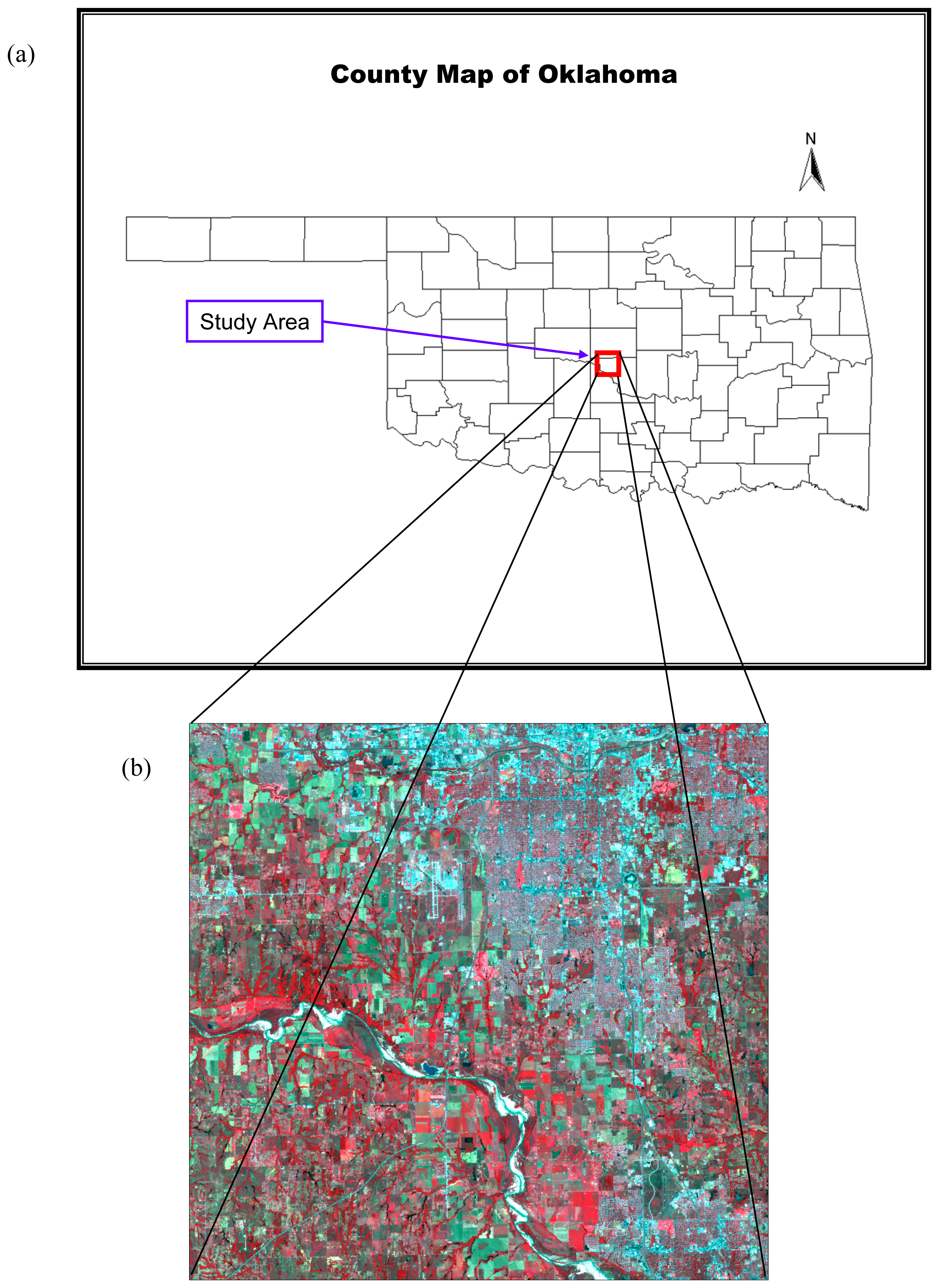
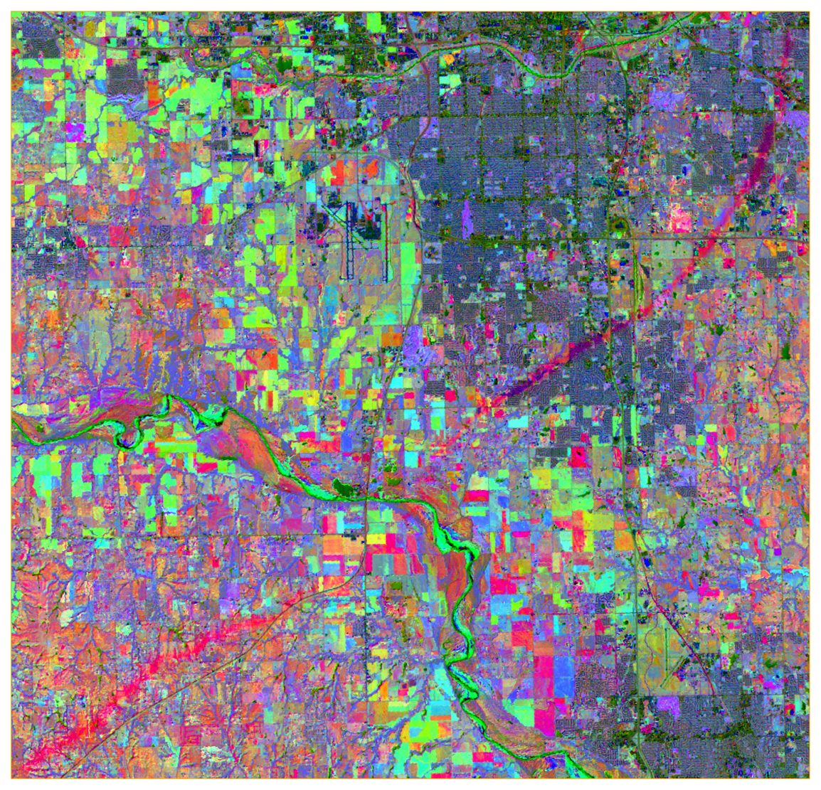
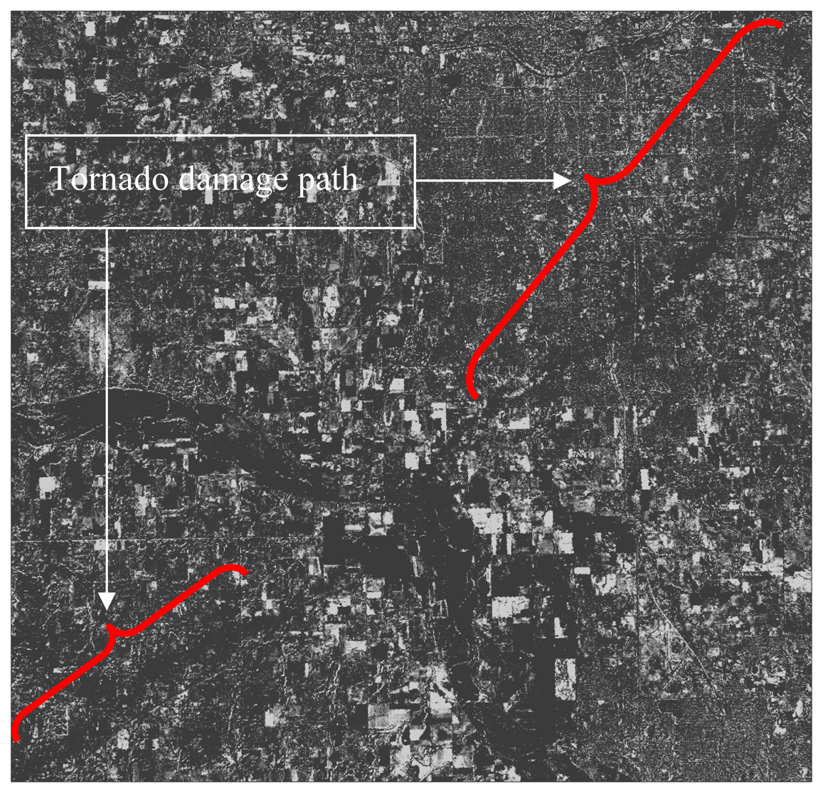
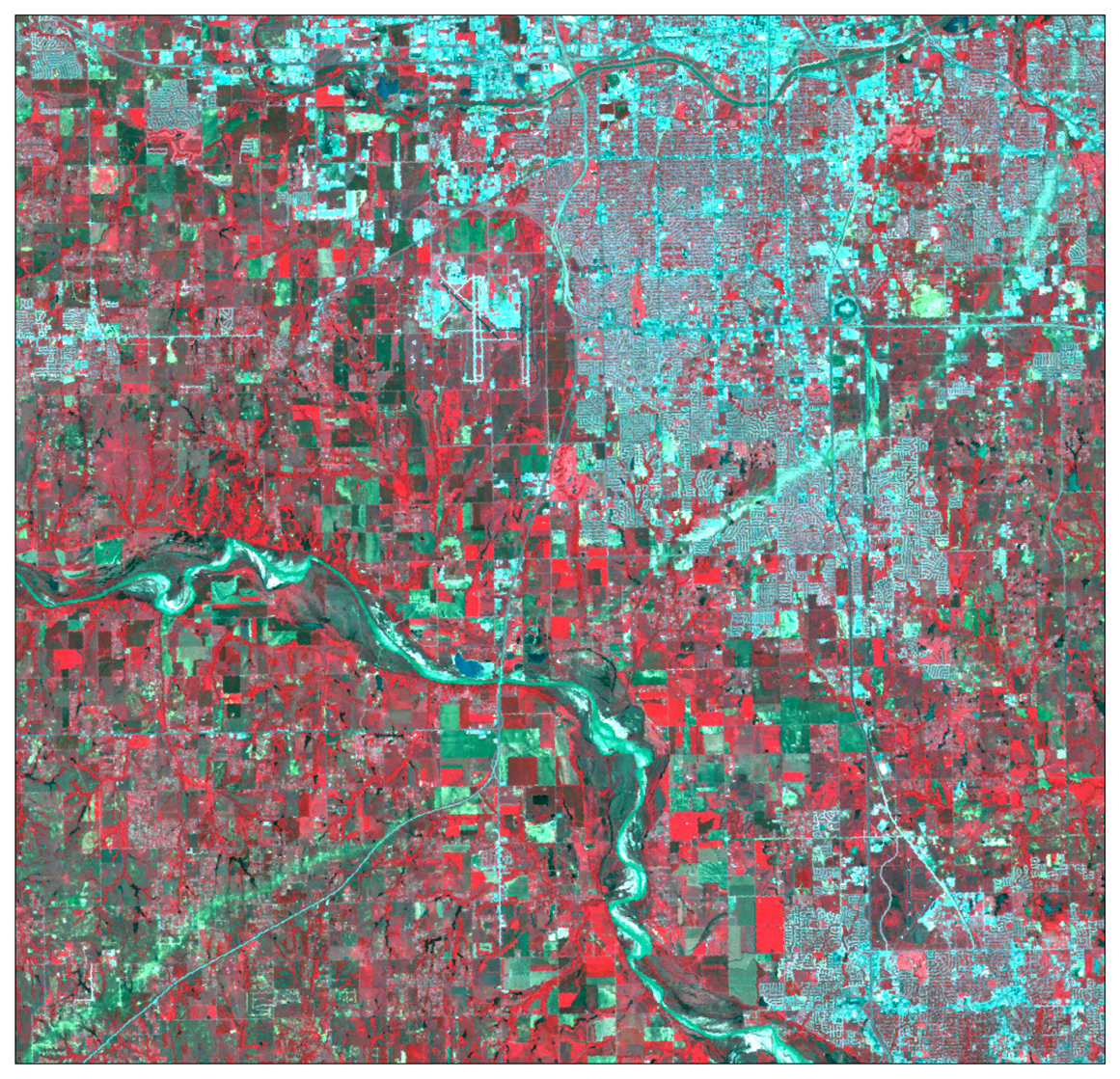
Figure 1.
(a) Location map of the study area; (b) A false color composite of the study area (June 26, 1998) displaying channel 4 (0.76 - 0.90 μm) in red, channel 3 (0.63 – 0.69 μm) in green, and channel 2 (0.52 – 0.60 μm) in blue.
Figure 1.
(a) Location map of the study area; (b) A false color composite of the study area (June 26, 1998) displaying channel 4 (0.76 - 0.90 μm) in red, channel 3 (0.63 – 0.69 μm) in green, and channel 2 (0.52 – 0.60 μm) in blue.
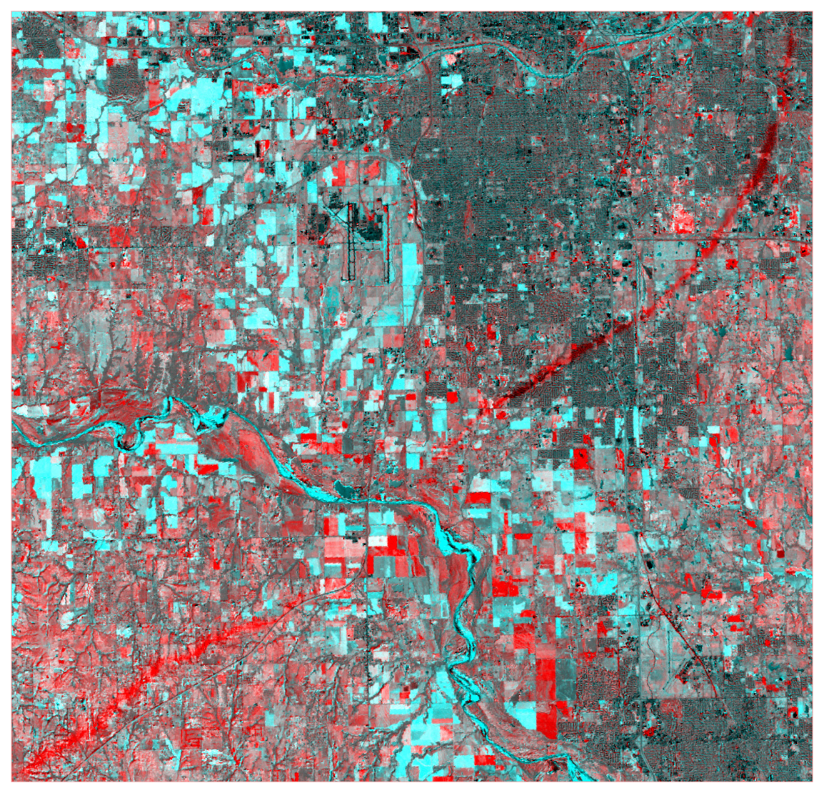
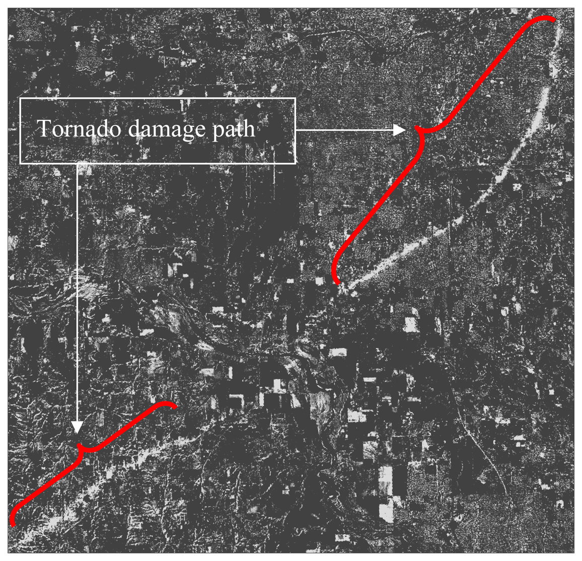
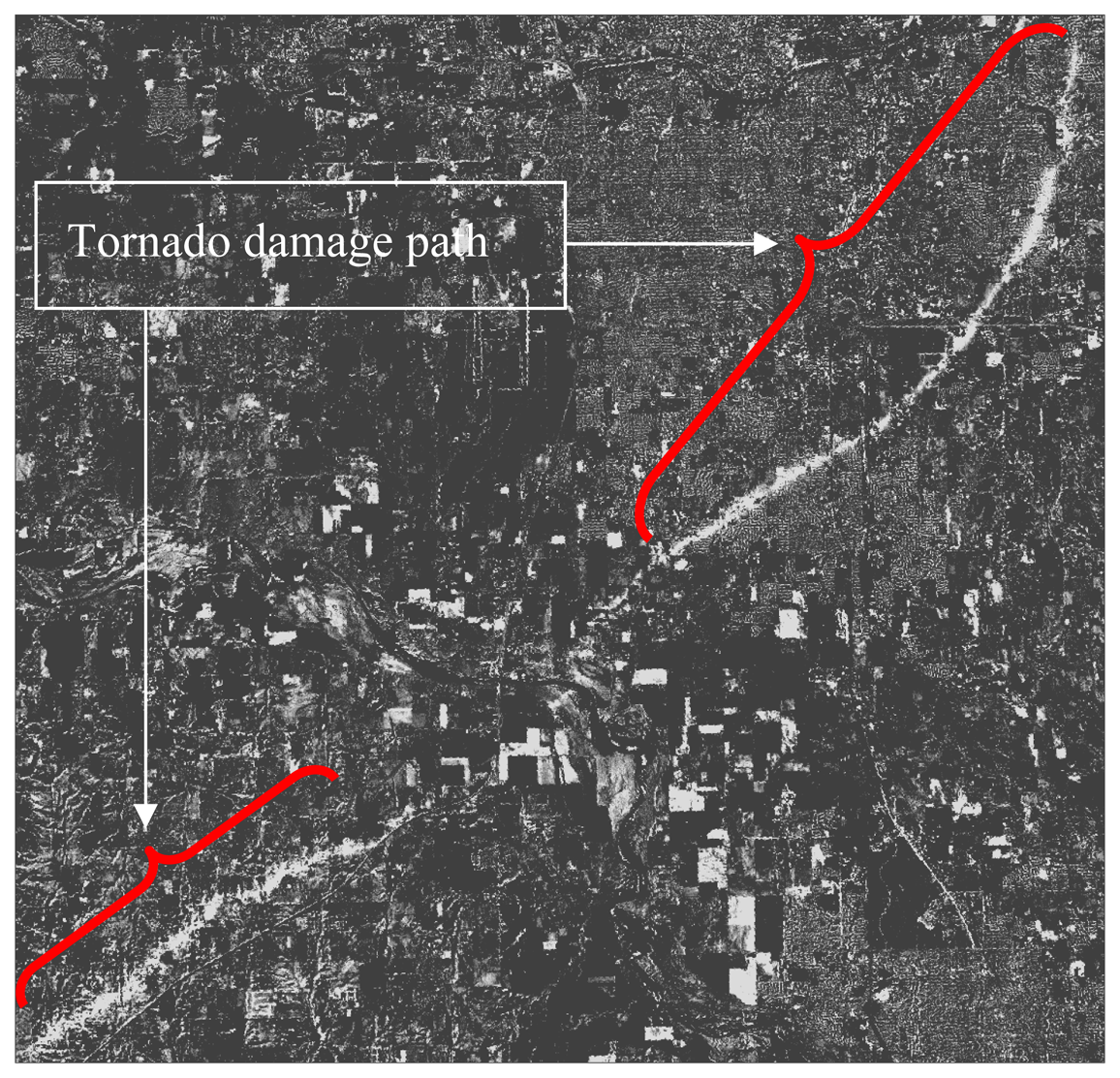
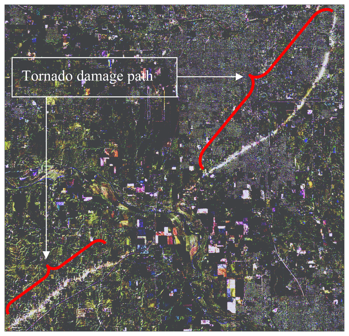
Figure 2.
A false color composite of the study area (May 12, 1999) displaying channel 4 (0.76 – 0.90 μm) in red, channel 3 (0.63 – 0.69 μm) in green, and channel 2 (0.52 – 0.60 μm) in blue.
Figure 2.
A false color composite of the study area (May 12, 1999) displaying channel 4 (0.76 – 0.90 μm) in red, channel 3 (0.63 – 0.69 μm) in green, and channel 2 (0.52 – 0.60 μm) in blue.
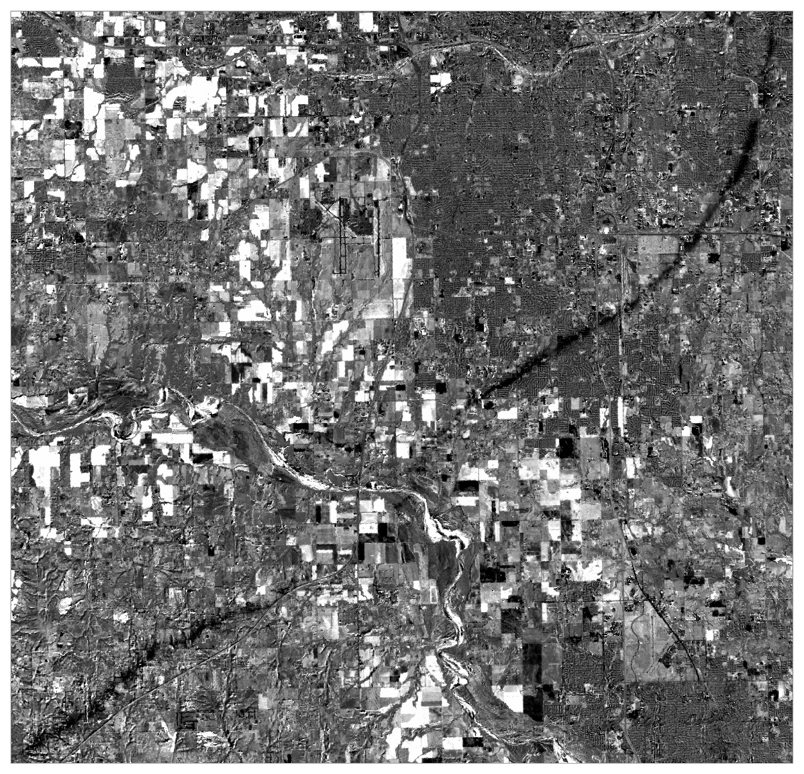
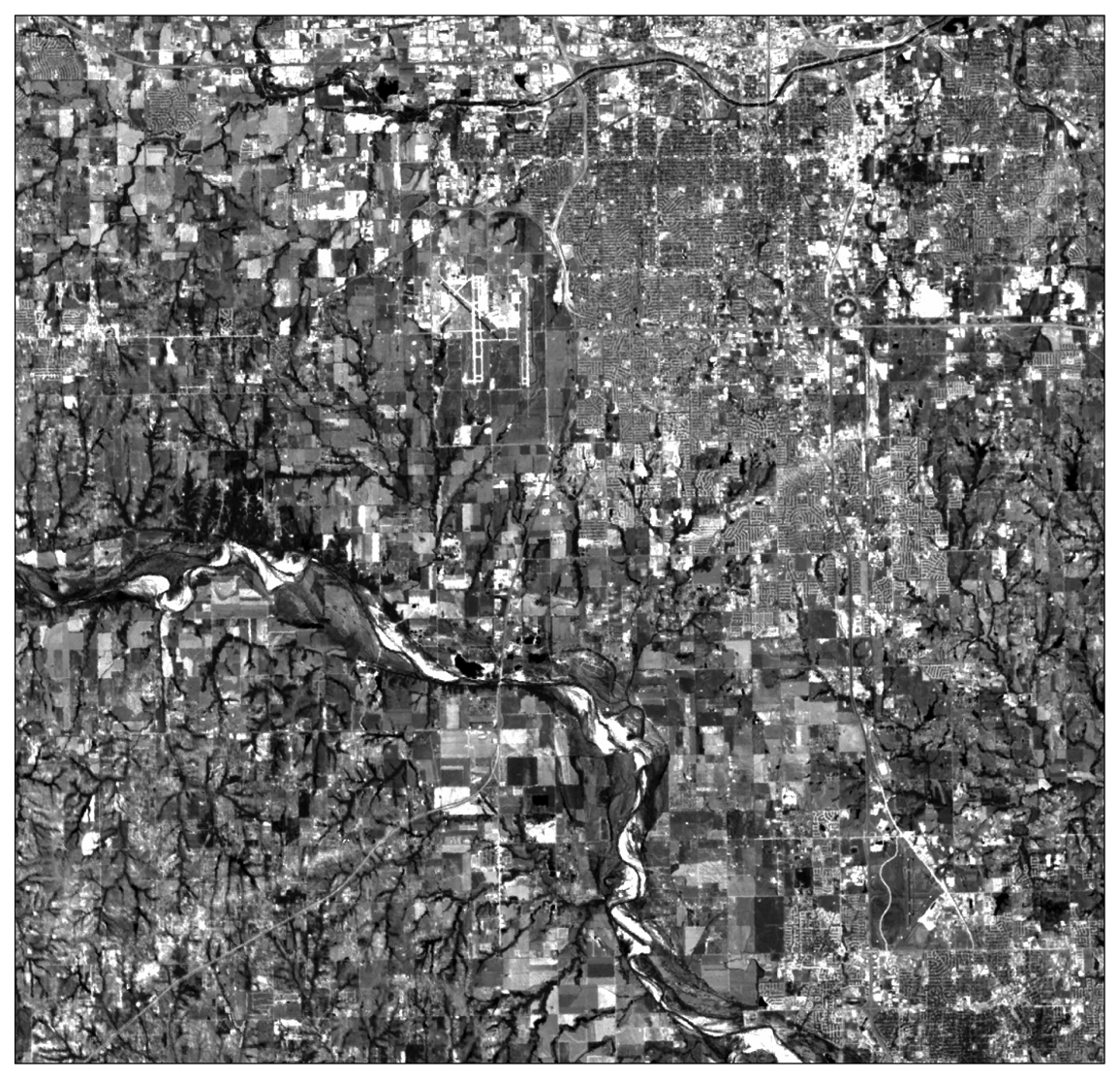
Figure 3.
Principal component composite band 1.
Figure 3.
Principal component composite band 1.
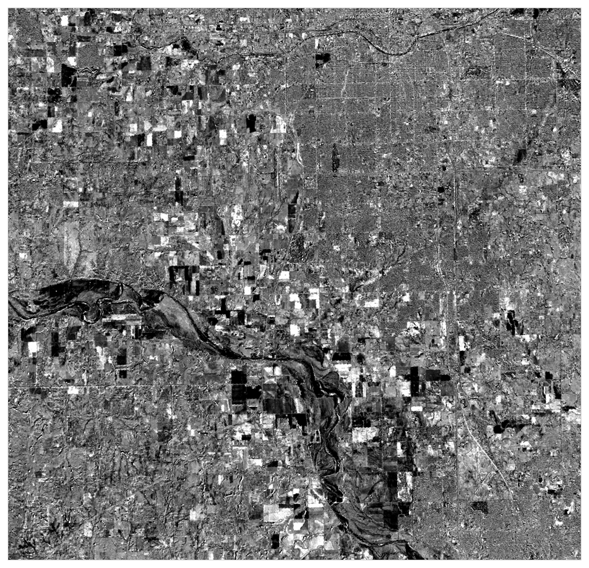
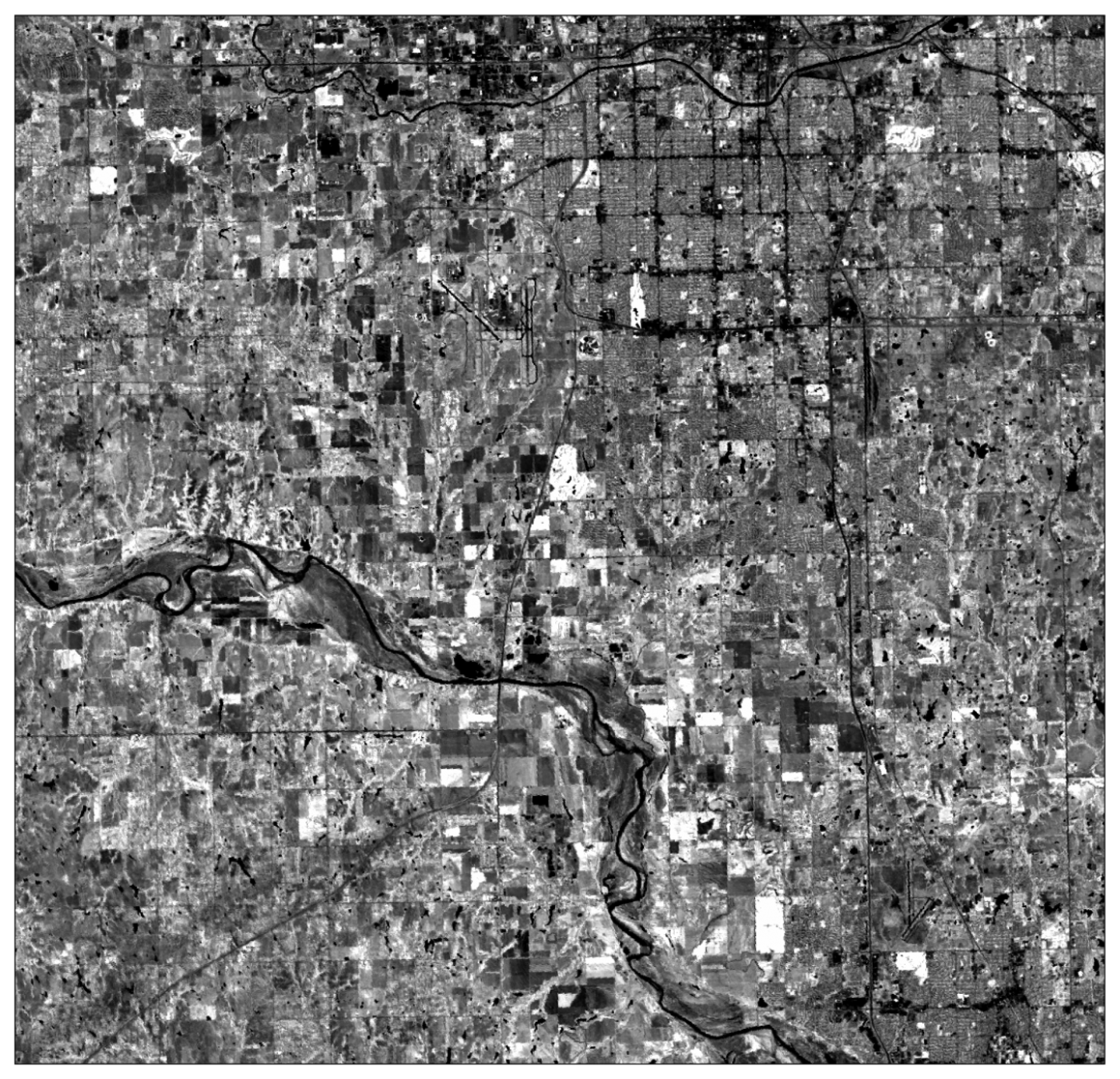
Figure 4.
Principal component composite band 2.
Figure 4.
Principal component composite band 2.
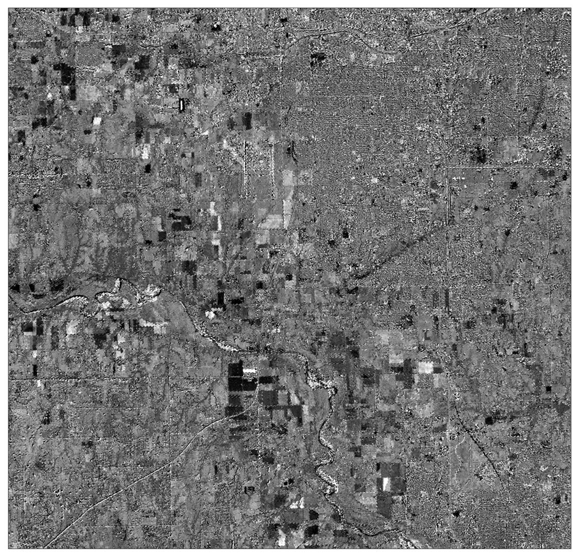
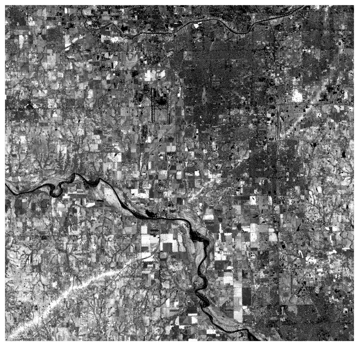
Figure 5.
Principal component composite band 3.
Figure 5.
Principal component composite band 3.
Figure 6.
Principal component composite band 4.
Figure 6.
Principal component composite band 4.
Figure 7.
Principal component composite band 5.
Figure 7.
Principal component composite band 5.
Figure 8.
Principal component composite band 6.
Figure 8.
Principal component composite band 6.
Figure 9.
Principal component composite bands 2, 3, and 4.
Figure 9.
Principal component composite bands 2, 3, and 4.
Figure 10.
Principal component composite bands 3 and 4.
Figure 10.
Principal component composite bands 3 and 4.
Figure 11.
Image difference band 1.
Figure 11.
Image difference band 1.
Figure 12.
Image difference band 2.
Figure 12.
Image difference band 2.
Figure 13.
Image difference band 3.
Figure 13.
Image difference band 3.
Figure 14.
Image difference band 4.
Figure 14.
Image difference band 4.
Figure 15.
Image difference band 5.
Figure 15.
Image difference band 5.
Figure 16.
Image difference band 7.
Figure 16.
Image difference band 7.
Figure 17.
Image difference bands 3, 5, and 7
Figure 17.
Image difference bands 3, 5, and 7
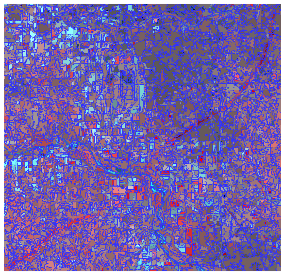
Figure 18.
A segmented image of PC composite bands 3 and 4 using shape (Ssh) 0.3, compactness (Scm) 0.5, and scale (Ssc) 100.
Figure 18.
A segmented image of PC composite bands 3 and 4 using shape (Ssh) 0.3, compactness (Scm) 0.5, and scale (Ssc) 100.
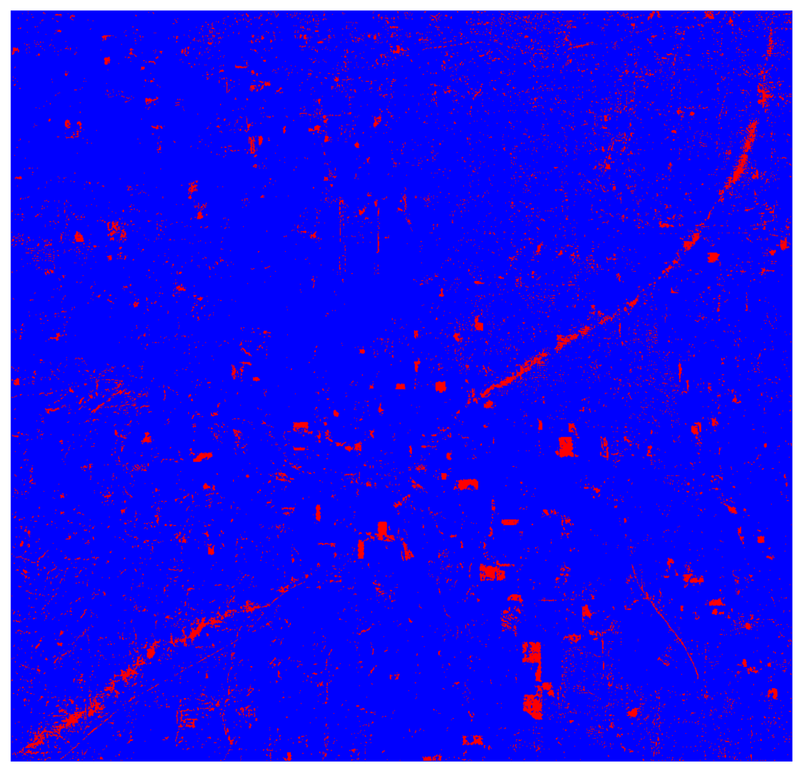
Figure 19.
An output map of PC composite bands 2, 3, and 4 using an unsupervised approach (i.e., ISODATA). Note: blue color represents non-damaged areas and red color represents damaged areas.
Figure 19.
An output map of PC composite bands 2, 3, and 4 using an unsupervised approach (i.e., ISODATA). Note: blue color represents non-damaged areas and red color represents damaged areas.
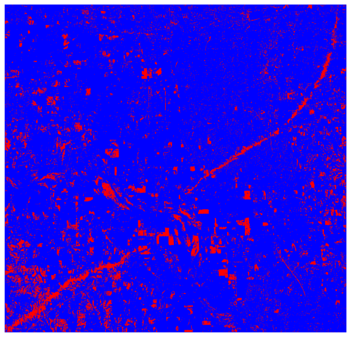
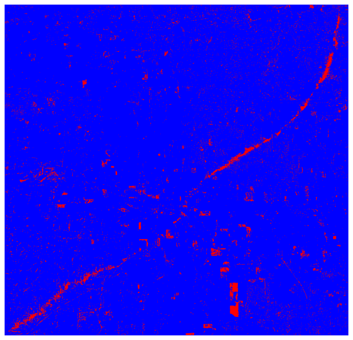
Figure 20.
An output map of PC composite bands 2, 3, and 4 using a supervised approach (i.e., maximum likelihood). Note: blue color represents non-damaged areas and red color represents damaged areas.
Figure 20.
An output map of PC composite bands 2, 3, and 4 using a supervised approach (i.e., maximum likelihood). Note: blue color represents non-damaged areas and red color represents damaged areas.
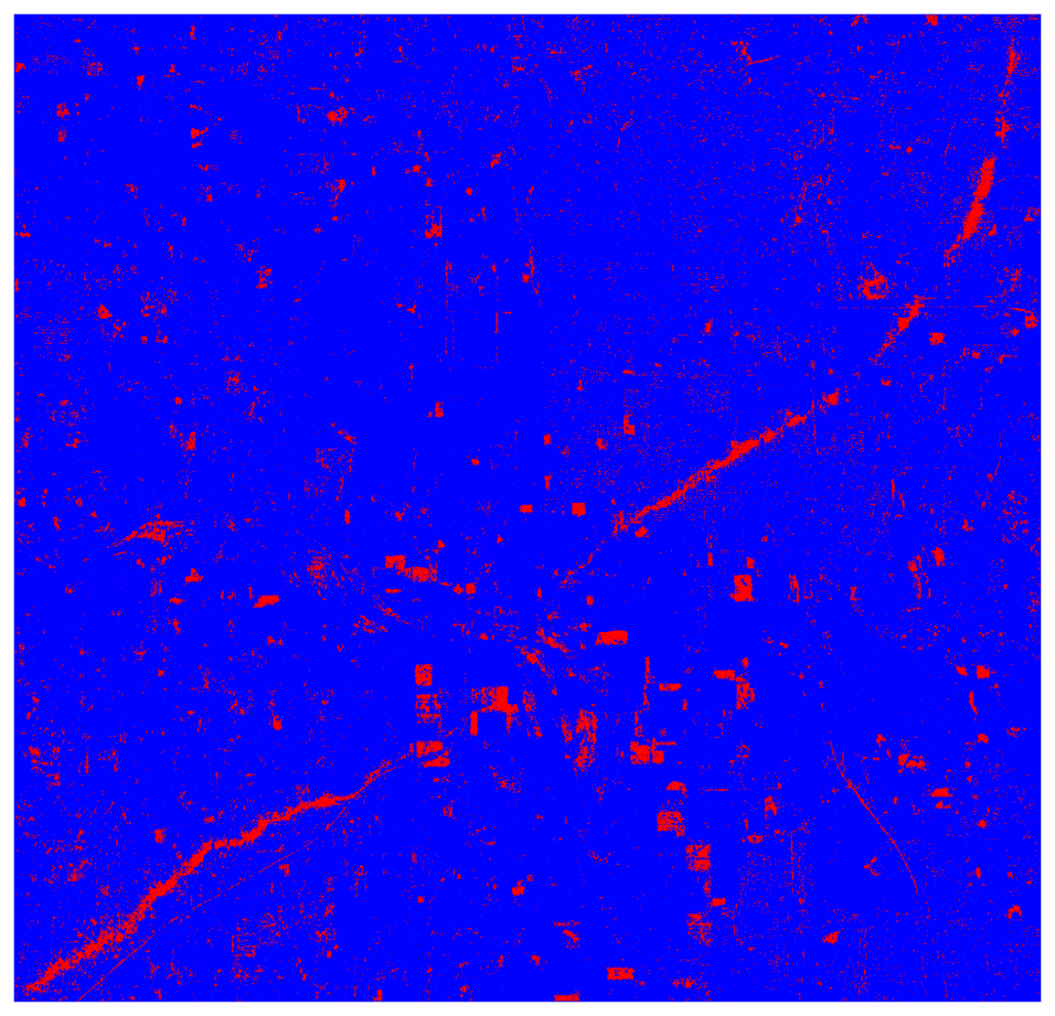
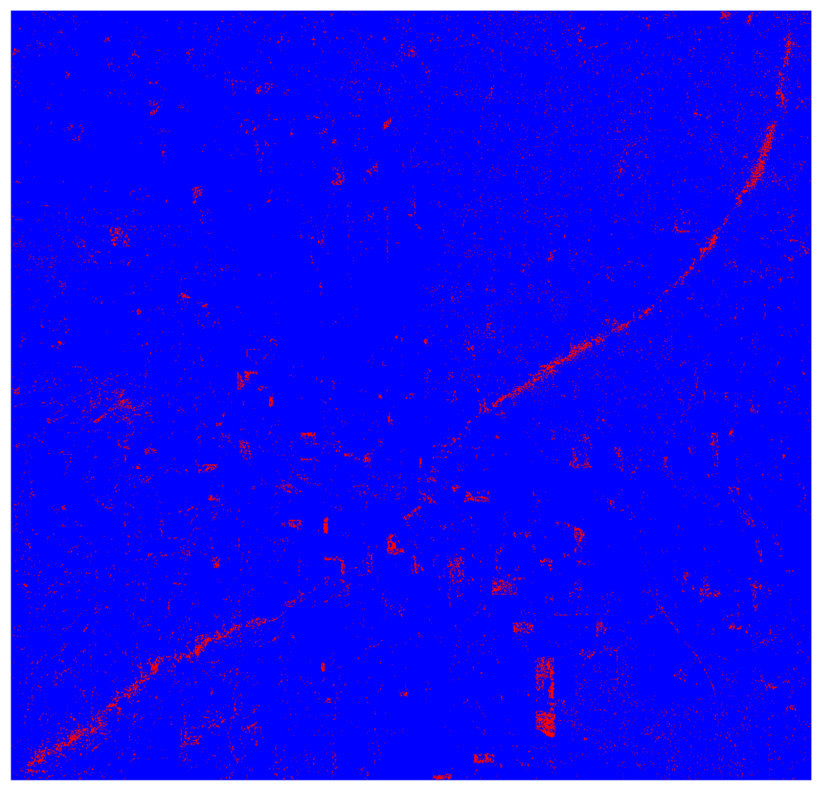
Figure 21.
An output map of PC composite bands 3 and 4 using an unsupervised approach (i.e., ISODATA). Note: blue color represents non-damaged areas and red color represents damaged areas.
Figure 21.
An output map of PC composite bands 3 and 4 using an unsupervised approach (i.e., ISODATA). Note: blue color represents non-damaged areas and red color represents damaged areas.
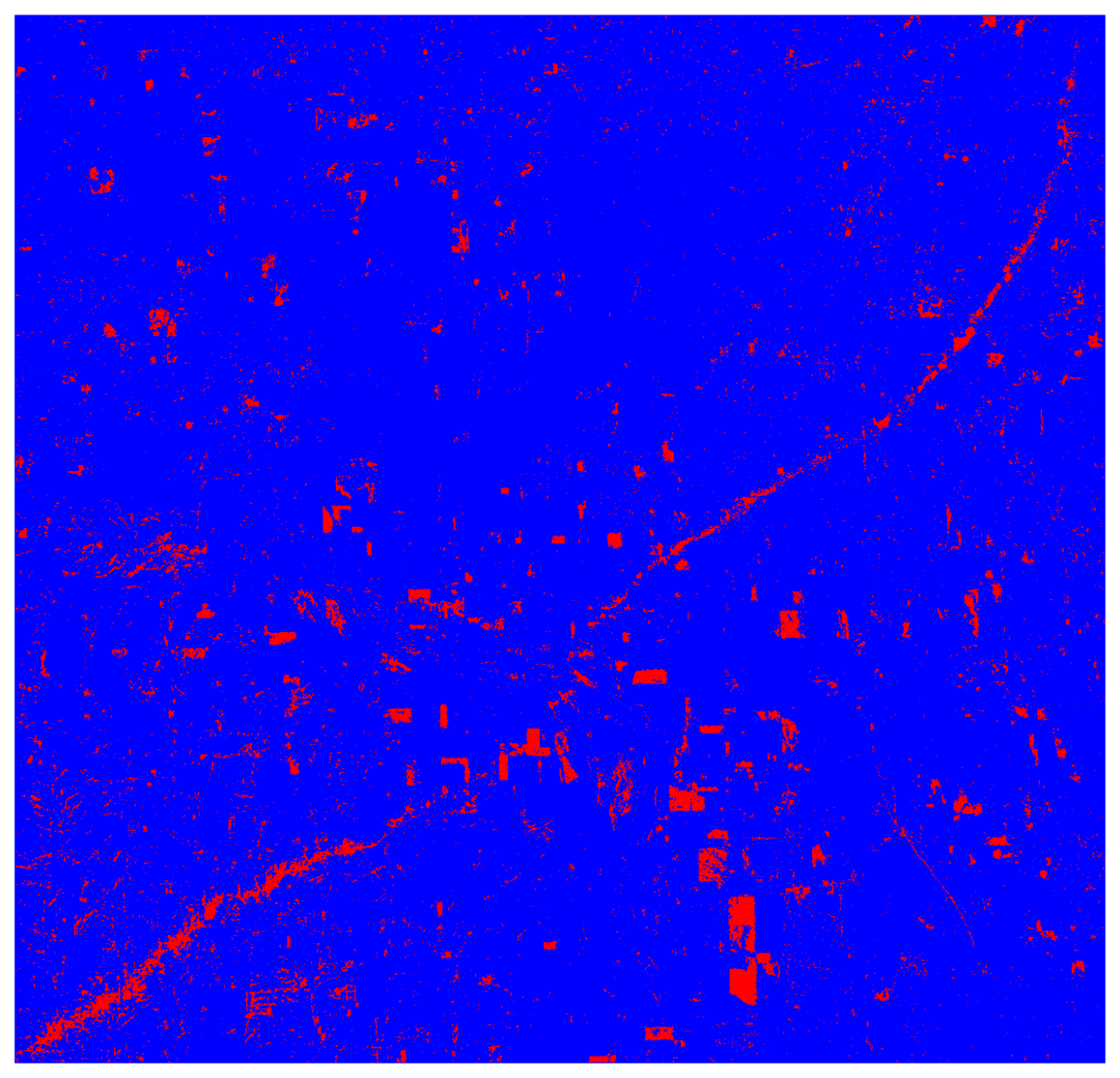
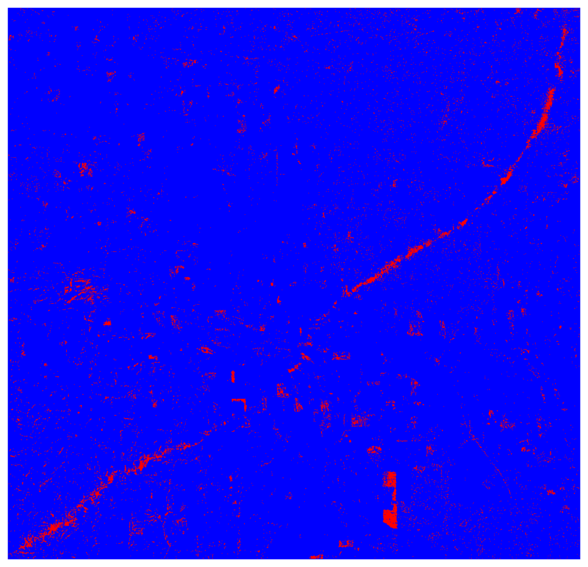
Figure 22.
An output map of PC composite bands 3 and 4 using a supervised approach (i.e., maximum likelihood). Note: blue color represents non-damaged areas and red color represents damaged areas.
Figure 22.
An output map of PC composite bands 3 and 4 using a supervised approach (i.e., maximum likelihood). Note: blue color represents non-damaged areas and red color represents damaged areas.
Figure 23.
An output map of image difference bands 1, 2, 3, 4, 5, and 7 using an unsupervised approach (i.e., ISODATA). Note: blue color represents non-damaged areas and red color represents damaged areas.
Figure 23.
An output map of image difference bands 1, 2, 3, 4, 5, and 7 using an unsupervised approach (i.e., ISODATA). Note: blue color represents non-damaged areas and red color represents damaged areas.
Figure 24.
An output map of image difference bands 1, 2, 3, 4, 5, and 7 using a supervised approach (i.e., maximum likelihood). Note: blue color represents non-damaged areas and red color represents damaged areas.
Figure 24.
An output map of image difference bands 1, 2, 3, 4, 5, and 7 using a supervised approach (i.e., maximum likelihood). Note: blue color represents non-damaged areas and red color represents damaged areas.
Figure 25.
An output map of image difference bands 3, 5, and 7 using an unsupervised approach (i.e., ISODATA). Note: blue color represents non-damaged areas and red color represents damaged areas.
Figure 25.
An output map of image difference bands 3, 5, and 7 using an unsupervised approach (i.e., ISODATA). Note: blue color represents non-damaged areas and red color represents damaged areas.
Figure 26.
An output map of a image difference bands 3, 5, and 7 using a supervised approach (i.e., maximum likelihood). Note: blue color represents non-damaged areas and red color represents damaged areas.
Figure 26.
An output map of a image difference bands 3, 5, and 7 using a supervised approach (i.e., maximum likelihood). Note: blue color represents non-damaged areas and red color represents damaged areas.
Figure 27.
An output map of PC composite bands 3 and 4 using an object oriented approach. Note: The output image was not manually edited or filtered.
Figure 27.
An output map of PC composite bands 3 and 4 using an object oriented approach. Note: The output image was not manually edited or filtered.
Table 1.
Overall accuracy, producer's accuracy, user's accuracy, and Kappa coefficient produced by a composite image of PC bands 2, 3, and 4 with an unsupervised classifier (i.e., ISODATA).
Table 1.
Overall accuracy, producer's accuracy, user's accuracy, and Kappa coefficient produced by a composite image of PC bands 2, 3, and 4 with an unsupervised classifier (i.e., ISODATA).
| Classified | Reference | Total | Producer's Accuracy | User's Accuracy |
|---|
|
|---|
| Non-Damaged | Damaged |
|---|
| Non-Damaged | 67 | 14 | 81 | 93.06% | 87.72% |
| Damaged | 5 | 34 | 39 | 70.83% | 87.18% |
|
| Total | 72 | 48 | 120 | | |
Table 2.
Overall accuracy, producer's accuracy, user's accuracy, and Kappa coefficient produced by a composite image of PC bands 2, 3, and 4 with a supervised classifier (i.e., maximumlikelihood).
Table 2.
Overall accuracy, producer's accuracy, user's accuracy, and Kappa coefficient produced by a composite image of PC bands 2, 3, and 4 with a supervised classifier (i.e., maximumlikelihood).
| Classified | Reference | Total | Producer's Accuracy | User's Accuracy |
|---|
|
|---|
| Non-Damaged | Damaged |
|---|
| Non-Damaged | 72 | 25 | 97 | 100.00% | 74.23% |
| Damaged | 0 | 23 | 23 | 47.92% | 100.00% |
|
| Total | 72 | 48 | 120 | | |
Table 3.
Overall accuracy, producer's accuracy, user's accuracy, and Kappa coefficient produced by a composite image of PC bands 3 and 4 with an unsupervised classifier (i.e., ISODATA).
Table 3.
Overall accuracy, producer's accuracy, user's accuracy, and Kappa coefficient produced by a composite image of PC bands 3 and 4 with an unsupervised classifier (i.e., ISODATA).
| Classified | Reference | Total | Producer's Accuracy | User's Accuracy |
|---|
|
|---|
| Non-Damaged | Damaged |
|---|
| Non-Damaged | 72 | 17 | 89 | 91.03% | 89.87% |
| Damaged | 1 | 30 | 31 | 80.95% | 82.93% |
|
| Total | 73 | 47 | 120 | | |
Table 4.
Overall accuracy, producer's accuracy, user's accuracy, and Kappa coefficient produced by a composite image of PC bands 3 and 4 with a supervised classifier (i.e., maximumlikelihood).
Table 4.
Overall accuracy, producer's accuracy, user's accuracy, and Kappa coefficient produced by a composite image of PC bands 3 and 4 with a supervised classifier (i.e., maximumlikelihood).
| Classified | Reference | Total | Producer's Accuracy | User's Accuracy |
|---|
|
|---|
| Non-Damaged | Damaged |
|---|
| Non-Damaged | 71 | 8 | 79 | 91.03% | 89.87% |
| Damaged | 7 | 34 | 41 | 80.95% | 82.93% |
|
| Total | 78 | 42 | 120 | | |
Table 5.
Overall accuracy, producer's accuracy, user's accuracy, and Kappa coefficient produced by a composite image difference of the original reflectance bands 1, 2, 3, 4, 5, and 7 with an unsupervised classifier (i.e., ISODATA).
Table 5.
Overall accuracy, producer's accuracy, user's accuracy, and Kappa coefficient produced by a composite image difference of the original reflectance bands 1, 2, 3, 4, 5, and 7 with an unsupervised classifier (i.e., ISODATA).
| Classified | Reference | Total | Producer's Accuracy | User's Accuracy |
|---|
|
|---|
| Non-Damaged | Damaged |
|---|
| Non-Damaged | 73 | 23 | 96 | 100.00% | 76.04% |
| Damaged | 0 | 24 | 24 | 51.06% | 100.00% |
|
| Total | 73 | 47 | 120 | | |
Table 6.
Overall accuracy, producer's accuracy, user's accuracy, and Kappa coefficient produced by a composite image difference of the original reflectance bands 1, 2, 3, 4, 5, and 7 with a supervised classifier (i.e., maximumlikelihood).
Table 6.
Overall accuracy, producer's accuracy, user's accuracy, and Kappa coefficient produced by a composite image difference of the original reflectance bands 1, 2, 3, 4, 5, and 7 with a supervised classifier (i.e., maximumlikelihood).
| Classified | Reference | Total | Producer's Accuracy | User's Accuracy |
|---|
|
|---|
| Non-Damaged | Damaged |
|---|
| Non-Damaged | 73 | 17 | 90 | 96.05% | 81.11% |
| Damaged | 3 | 27 | 30 | 61.36% | 90.00% |
|
| Total | 76 | 44 | 120 | | |
Table 7.
Overall accuracy, producer's accuracy, user's accuracy, and Kappa coefficient produced by a composite image difference of the original reflectance bands 3, 5, and 7 with an unsupervised classifier (i.e., ISODATA).
Table 7.
Overall accuracy, producer's accuracy, user's accuracy, and Kappa coefficient produced by a composite image difference of the original reflectance bands 3, 5, and 7 with an unsupervised classifier (i.e., ISODATA).
| Classified | Reference | Total | Producer's Accuracy | User's Accuracy |
|---|
|
|---|
| Non-Damaged | Damaged |
|---|
| Non-Damaged | 73 | 35 | 108 | 100.00% | 67.59% |
| Damaged | 0 | 12 | 12 | 25.53% | 100.00% |
|
| Total | 73 | 47 | 120 | | |
Table 8.
Overall accuracy, producer's accuracy, user's accuracy, and Kappa coefficient produced by a composite image difference of the original reflectance bands 3, 5, and 7 with a supervised classifier (i.e., maximumlikelihood).
Table 8.
Overall accuracy, producer's accuracy, user's accuracy, and Kappa coefficient produced by a composite image difference of the original reflectance bands 3, 5, and 7 with a supervised classifier (i.e., maximumlikelihood).
| Classified | Reference | Total | Producer's Accuracy | User's Accuracy |
|---|
|
|---|
| Non-Damaged | Damaged |
|---|
| Non-Damaged | 73 | 26 | 99 | 100.00% | 73.74% |
| Damaged | 0 | 21 | 21 | 44.68% | 100.00% |
|
| Total | 73 | 47 | 120 | | |
Table 9.
Overall accuracy, producer's accuracy, user's accuracy, and Kappa coefficient produced by a composite image of PC bands 3 and 4 with an object-oriented approach.
Table 9.
Overall accuracy, producer's accuracy, user's accuracy, and Kappa coefficient produced by a composite image of PC bands 3 and 4 with an object-oriented approach.
| Classified | Reference | Total | Producer's Accuracy | User's Accuracy |
|---|
|
|---|
| Non-Damaged | Damaged |
|---|
| Non-Damaged | 73 | 2 | 75 | 100.00% | 97.33% |
| Damaged | 0 | 45 | 45 | 95.74% | 100.00% |
|
| Total | 73 | 47 | 120 | | |


