VLF/LF Radio Sounding of Ionospheric Perturbations Associated with Earthquakes

Department of Electronic Engineering and Research Station on Seismo Electromagnetics, The University of Electro-Communications, 1-5-1 Chofugaoka, Chofu, Tokyo 182-8585, Japan
Sensors 2007, 7(7), 1141-1158; https://doi.org/10.3390/s7071141
Submission received: 18 June 2007
/
Accepted: 5 July 2007
/
Published: 10 July 2007
(This article belongs to the Special Issue Sensors for Disaster and Emergency Management Decision Making)
Abstract
:It is recently recognized that the ionosphere is very sensitive to seismic effects, and the detection of ionospheric perturbations associated with earthquakes, seems to be very promising for short-term earthquake prediction. We have proposed a possible use of VLF/LF (very low frequency (3-30 kHz) /low frequency (30-300 kHz)) radio sounding of the seismo-ionospheric perturbations. A brief history of the use of subionospheric VLF/LF propagation for the short-term earthquake prediction is given, followed by a significant finding of ionospheric perturbation for the Kobe earthquake in 1995. After showing previous VLF/LF results, we present the latest VLF/LF findings; One is the statistical correlation of the ionospheric perturbation with earthquakes and the second is a case study for the Sumatra earthquake in December, 2004, indicating the spatical scale and dynamics of ionospheric perturbation for this earthquake.
1. Introduction to Seismo Electromagnetics
There have been a wide variety of natural disasters including abnormal meteorological effects (abnormal climate changes), earthquakes, volcano eruption, etc. In this review we deal only with earthquakes, and the media news for the latest, huge earthquakes such as Japanese Niigata earthquake, Indonesia Sumatra earthquake etc. have indicated how large the earthquake hazard is. In order to mitigate the earthquake disaster, the earthquake prediction is of primary importance. Generally speaking, the earthquake prediction can be classified into three, depending on the time scale we are concerned with. Due to the enormous advance in seismogology, seismic geology and geodesy, we notice significant achievement in (1) long-term (of the order of a few hundred years) and (2) medium-term (of the order of hundreds to a few years) prediction. However, in sprite of the essential importance of (3) short-term (of the order of a few months to a few days) earthquake prediction, it has been far from realization. The situation for the short-term earthquake prediction seems to have drastically changed during the last ten years since the Kobe earthquake in 1995. The conventional earthquake prediction has been based on the measurement of crustal movement, but this kind of mechanical measurement has been concluded to be not so useful in the short-term earthquake prediction. Then, we have had a new wave of the measurements by means of electromagnetic effects, and we have accumulated a lot of evidence that electromagnetic phenomena take place in a wide frequency range prior to an earthquake (e.g., Hayakawa, 1999; Hayakawa and Molchanov, 2002). While the mechanical effect provides us with the 0th-order (or macroscopic) information on the lithosphere, the higher-order (microscopic) information can only be tackled by electromagnetic effects.
The electromagnetic method for earthquake prediction can principally be classified into two categories: The first is the detection of radio emissions from the hypocenter, and the second is to detect an indirect effect of earthquakes taking place in the atmosphere and ionosphere by means of the preexisting radio transmitter signals (we call it “radio sounding”). As the result of research during the last ten years, it has been a consensus that the ionosphere is unexpectedly extremely sensitive to the seismic effect (e.g., Hayakawa and Molchanov, 2002), which is the topic of this review.
2. VLF/LF radio sounding of ionospheric perturbations associated with earthquakes: Previous works
2.1. The use of VLF/LF subionospheric propagation as new methodology
A number of nations currently operate large VLF/LF transmitters primarily for navigation and communication with military submarines. To radiate electromagnetic waves efficiently, one needs an antenna with dimensions on the order of a wavelength of the radiation, which suggests that VLF/LF transmitter antennas are very large, typically many hundreds of meters high.
Most of the energy radiated by such VLF/LF transmitters is trapped between the ground and the lower ionosphere, forming the Earth-ionosphere waveguide. Subionospheric VLF/LF signals reflect from the D-region of the ionosphere, probably the least studied region of the Earth's atmosphere. These altitudes (∼ 70-90 km) are too far for balloons and too low for satellites, making in-situ measurements extremely rare. The only possible method of probing this D region is VLF/LF subionospheric radio signals.
Any variations on the ionospheric D/E-region lead to changes in the propagation conditions for VLF waves propagating subionospherically, and hence changes in the observed amplitude and phase of VLF/LF transmissions are due to different kinds of perturbation sources; (1) solar flares, (2) geomagnetic storms (and the corresponding particle precipitation), (3) the direct effect of lightning (e.g., Rodgers and McCormic, 2006). In addition to these solar-terrestrial effects we can suggest one more effect of earthquakes (or seismic activity) onto the lower ionosphere.
2.2. Previous works
The first attempt of VLF/LF radio sounding for seismo-ionospheric effects was done by Russian colleagues (Gokhberg et al., 1989; Gufeld et al., 1992), who studied the VLF propagaton over a long distance from Reunion (Omega transmitter) to Omsk to detect any effect of an earthquake in the Caucasia region. Then, they succeeded in finding out a significant propagation anomaly over the two long-distance paths from Reunion to Moscow and also to Omsk a few days before the famous Spitak earthquake (Gufeld et al., 1992).
The most convincing result on the seismo-ionospheric perturbations with VLF sounding was obtained by Hayakawa et al. (1996) for the famous Kobe earthquake in 1995 (with magnitude of 7.3 and with depth of 20 km). Some important peculiarities in their paper are summarized as follows; (1) the propagation distance (from Tsushima Omega to Inubo observatory) is relatively short-path at VLF (∼ 1,000 km) as shown in Fig. 1(a), as compared with 5,000 ∼ 9,000 km used in Russian papers (Gokhberg et al., 1989; Gufeld et al., 1992), and (2) they found that the fluctuation method as used before, was not so effective for the short-propagation path, so that they developed another way of analysis. That is, they paid attention to the times of terminator (morning and evening) and they found significant shifts in the terminator times before the earthquake, as shown in Fig. 1(b). The morning terminator time (tm) shifts to early hours, and te shifts to later hours. This point was statistically examined by a much longer data-base of ±4 months, which indicates that the shift in te (phase) in Fig 1(b) is found to exceed well above twice the standard deviation (2σ). This means that the daytime felt by subionospheric VLF signals is elongated for a few days around the earthquake, and the theoretical estimation (Hayakawa et al., 1996; Molchanov et al., 1998; Yamauchi et al., 2007) suggests that the lower ionosphere is lowered before the earthquake.
A later extensive study by Molchanov and Hayakawa (1998) was based on the much more events during 13 years (11 events with magnitude greater than 6.0 and within the 1st Fresnel zone) for the same propagation path from the Omega, Tsushima to Inubo, and they came to the following conclusion.
- (1)
- As for shallow (depth smaller than 30 km) earthquakes, 4 earthquakes form 5, exhibited the same terminator time anomaly as for the Kobe earthquake (as in Fig. 1(b)) (with the same 2 σ criterion).
- (2)
- When the depth of earthquakes is in a medium range of 30-100 km, there were observed two events. One event exhibited the same terminator time anomaly, and another indicated a different type of anomaly.
- (3)
- Deep (depth larger than 100 km) earthquakes (4 events) did not show any anomaly. Two of them had an extremely large magnitude (greater than 7.0), but had no propagation anomaly.
This summary might indicate a relatively high probability of the propagation anomaly (in the form of terminator time anomaly) of the order of 70 ∼ 80 % for larger (magnitude greater than 6.0) earthquakes located relatively close to the great-circle path (e.g., 1st Fresnel zone).
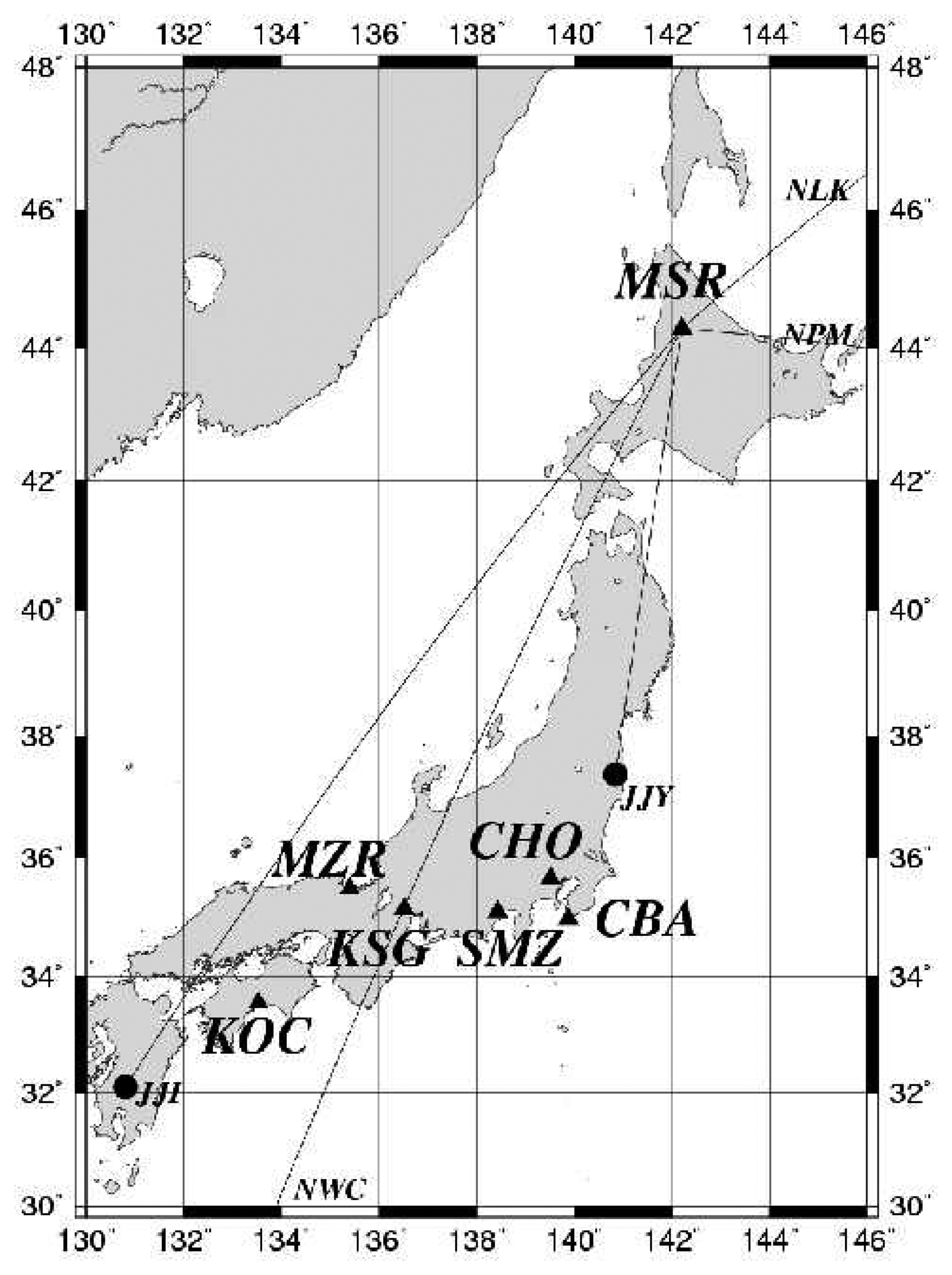
In response to the above –mentioned significant results (especially the result for Kobe earthquake), the Japanese government conducted the integrated earthquake frontier project, and the former NASDA (National Space Development Agency of Japan) conducted the so-called “Earthquake Remote Sensing Frontier Project” (for which the author was the principal investigator) during 1997 to 2001 (five years project) (Hayakawa et al., 2004a, b; Hayakawa, 2004). In this project our greatest attention was paid to the subionospheric VLF/LF propagation aimed at the short-term earthquake prediction. Fig. 2 is the Japanese VLF/LF network established within the framework of the Frontier Project and is still working. There are seven observing stations (Moshiri (Hokkaido), Chofu (Tokyo), Tateyama (Chiba), Shimizu (Shizuoka), Kasugai (Nagoya), Maizuru (Kyoto) and Kochi), and we observe several transmitters simultaneously at each station, unlike the early VLF receiving system. The VLF/LF transmitters now we observe, are (1) JJY (40 kHz, Fukushima), (2) JJI (22.2 kHz, Ebino, Kyushu), (3) NWC (19.8 kHz, Australia), (4) NPM (21.4 kHz, Hawaii) and (5) NLK (24.8 kHz, America). By using the combination of a number of observing stations and a large number of VLF/LF transmitters received, we will be able to locate the ionospheric perturbation with the accuracy of about 100 km. We make some comments on our Japal system. Our VLF/LF receiver named Japal, is designed to measure very slow and small changes in amplitude and phase. The magnitude of slow phase and amplitude perturbations claimed for earthquake precursors are much greater than this, so it should be detectable by our system if they exist.
Our VLF/LF system is deployed in different counties as well in response to their requests. One of our VLF/LF receivers is now working at Kamchatka in Russian with good data (Rozhnoi et al., 2004), and one is set in Taiwan as well. These stations, together with our Japanese dense network, are forming a global Pacific VLF/LF network. Additionally, a few VLF/LF receivers were installed in South Europe, and especially one in Italy is working good with significant results (Biagi et al., 2004).
By means of the above-mentioned Japanese VLF/LF network, we have been working on many case studies for large earthquakes. We can list these earthquakes; (1) Izu peninsula earthquake swarm (with the largest magnitude of 6.3) in March, 1997 (with the data from Tsushima, Omega to Chofu), (2) Tokai (Nagoya) area earthquakes (with data from NWC (Australia) to Kasugai (Nagoya) (Ohta et al., 2000), (3) Tokachi-oki earthquake (25 September, 2003, M8.3) (Shvets et al., 2004a; Cervone et al., 2006), (4) Niigata-chuetsu earthquakes (23 October, 2004, M6.8) (Hayakawa et al., 2006; Yamauchi et al., 2007). Especially, in the case of Niigata earthquake, we have made full use of our VLF/LF network observation (Yamauchi et al., 2007). That is, a comparison of the data on different propagation paths as a combination of several observing stations and several VLF/LF transmitter signals received, has enabled us to locate the ionospheric perturbation and to deduce their spatial scale. Also, their temporal dynamics have been inferred, together with the theoretical full-wave computations.
The terminator time method we developed, for the first rime, for the case of Kobe earthquake, has been used so far as a standard analysis method of VLF/LF records. In addition to this terminator time method, there is another method of VLF/LF data analysis, which is called, “nighttime fluctuation method” and which is a further improvement of the previous Russian papers.
3. Recent VLF/LF results
Here we present a few of our latest results by using our VLF/LF radio sounding. First, we present a result on the statistical correlation of ionospheric perturbations as detected by subionospheric VLF/LF radio sounding with the earthquakes. Then, we present a case study as detected in Japan for the huge Indonesia Sumatra earthquake.
3.1. Statistical study on the correlation between ionospheric perturbations and earthquakes
In addition to the event studies it is highly required to undertake any statistical study on the correlation between ionospheric disturbances and earthquakes based on abundant data source. There have been very few reports on the statistical correlation between the ionospherc perturbations and earthquakes (Shvets et al., 2002, 2004b; Rozhnoi et al., 2004). Shvets et al. (2004b) have examined a very short-period (March-August, 1997) data for two paths (one is the Tsushima-Chofu and another, NWC (Australia)-Chofu) and found that wave-like anomalies in VLF Omega signal with periods of a few hours (as indicative of the importance of atmospheric gravity wave as suggested by Molchanov et al., 2001; Miyaki et al., 2002) were observed 1-3 days before or on the day of moderately strong earthquakes with magnitudes 5-6.1. Then, Rozhnoi et al. (2004) have extensively studied 2 years data of the subionospheric LF signal along the path Japan (call sign, JJY)-Kamchatka (distance = 2,300 km), and have found from the statistical study that the LF signal effect is observed only for earthquakes with magnitude, at least, greater than 5.5.
The following is a summary of our latest paper (Maekawa et al., 2006) devoted to such a statistical study on the correlation between ionospheric disturbances and seismic activity. A few important distinction from the previous works by Shvets et al. (2002, 2004b) and Rozhnoi et al. (2004) are described. The first point is the use of much longer period of VLF/LF data (five years long). The second point is that we pay attention to physical parameters of VLF/LF propagation data; (1) amplitude (or trend) and (2) dispersion (in amplitude) (or fluctuation). In the previous work by Rozhnoi et al. (2004) they have studied the percentage occurrence of anomalous days, in which an anomalous day is defined as one day during which the difference of amplitude (and/or phase) from the monthly average exceeds one standard deviation (σ).
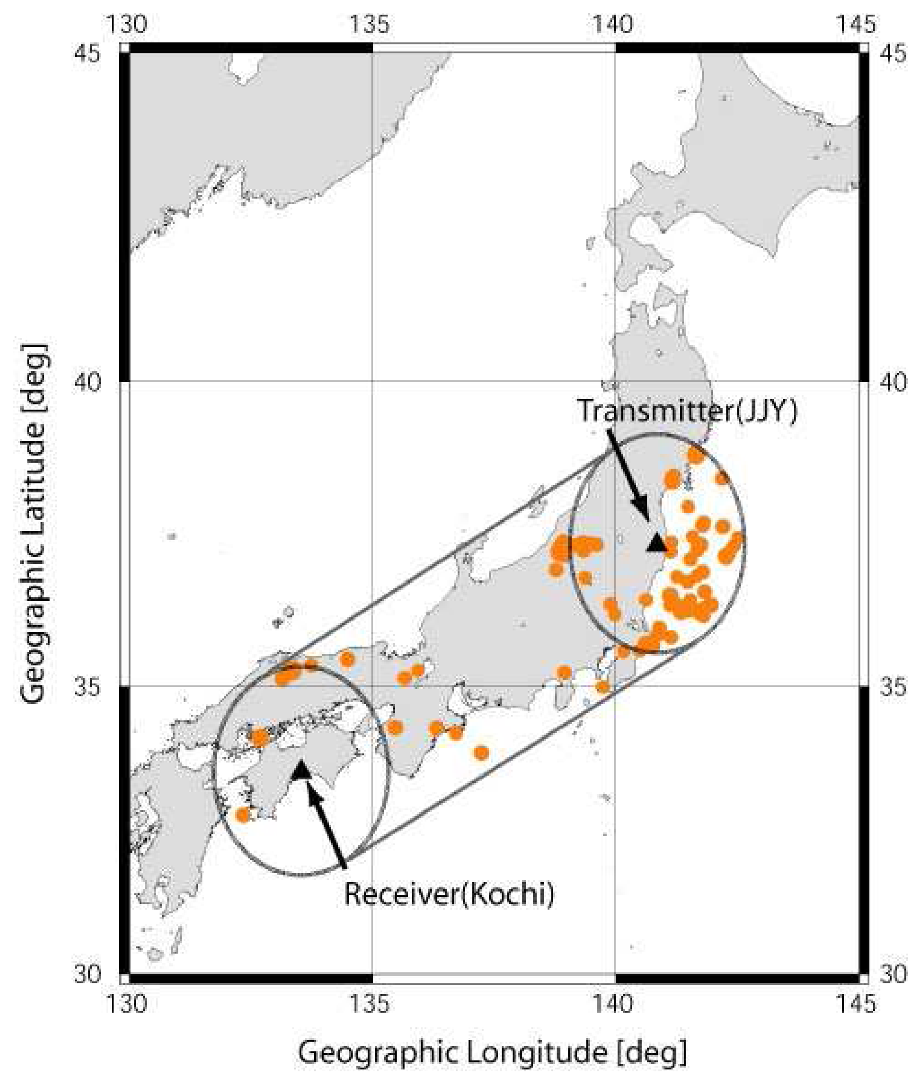
Here we pay particular attention to the earthquakes occurring in and around Japan, so that we take a wave path from the Japanese LF transmitter, JJY (40 kHz) (geographic coordinates; 36°18′ N, 139°85′ E) and a receiving station of Kochi (33°33′ N, 133°32′ E). Fig. 3 illustrates the relative location of the LF transmitter, JJY and our receiving station, Kochi, and the distance between the transmitter and receiver is 770 km.
The subionospheric LF data for this propagation path is taken over 6 years from June 1999 to June 2005, but we excluded one year of 2004 (January to December, 2004) because of the following reason. As you may know, there was an extremely large earthquake named 2004 Mid Niigata prefecture earthquake happened on October 23, with magnitude = 6.8 and depth = 10 km (Hayakawa et al., 2006), and the effect of the main shock and also large aftershocks was so large and so frequent that it may disturb our following statistical result so much. Then we have excluded this year of 2004 from our analysis. We have to define the criterion of choosing the earthquakes. The sensitive area for the wave path, JJY transmitter to the Kochi receiving station is defined as follows. As shown in Fig. 3, first we adopt the circles with radius of 200 km just around the transmitter and receiver, and then the sensitive area is defined by connecting the outer edges of these two circles. All of the 92 earthquakes with magnitude (conventional magnitude (M) by Japan Meteorological Agency) greater than 5.0 are plotted in Fig. 3, but the earthquake depth is chosen to be smaller than 100 km (with taking into account our previous result that shallow earthquakes can have an effect onto the ionosphere by Molchanov and Hayakawa (1998)). We have normally been using the fifth Fresnel zone as the VLF/LF sensitive area (Molchanov and Hayakawa, 1998; Rozhnoi et al., 2004), but we have found that the area just around the transmitter and receiver is also sensitive to VLF perturbation (e.g. Ohta et al., 2000) with taking into account the possible size of the seismo-ionospheric perturbation. In this sense the sensitive area we choose here seems to be very reasonable because the width of the sensitive area is very close to the 10th Fresnel zone.
In the following statistical analysis, we undertake the so-called superimposed epoch analysis in order to increase the S/N ratio. Here we define the earthquake magnitude in the following different way. Because we treat the data in the unit of one (a) day (we use U. T. (rather than L. T.) to count a day because we stay on the same day even when we pass the midnight when we use U.T.), we first estimate the total energy released from several earthquakes with different magnitudes in one day within the sensitive area for the LF wave path as shown in Fig. 3 by integrating the energy released by a few earthquakes (down to the conventional magnitude M = 2.0) and by converting this into an effective magnitude (Meff) for this particular day. This Meff is much more important than the conventional magnitude for each earthquake, because the LF propagation anomaly on one day is the effect integrated over several earthquakes taking place within the sensitive area on that day. Though not shown as a graph, we find that there are 19 days with Meff greater than 5.5.
Diurnal variations of the amplitude and phase of subionospheric VLF/LF signal are known to change significantly from month to month and from day to day. Therefore, following our previous works (Shvets et al., 2002, 2004a, b; Rozhnoi et al., 2004; Hayakawa et al., 2006; Horie et al., 2007a), we use, for our analysis, a residual signal of amplitude dA as the difference between the observed signal intensity (amplitude) and the average of several days preceding or following the current day:
where A(t) is the amplitude at a time t for a current day and <A(t) > is the corresponding average at the same time t for ±15 days (15 days before, 15 days after the earthquake and earthquake day). In the paper by Rozhnoi et al. (2004), they have defined an anomalous day when dA(t) exceeds the corresponding standard deviation. In our analysis we have studied the nighttime variation (in the U.T. range from U.T. = 10 h to 20 h) (or L.T. 19 h to 05 h)). Then, we use two physical parameters: average amplitude (we call it “amplitude”)(or trend) and amplitude dispersion (we call it “dispersion)(or fluctuation)). We estimate the average amplitude for each day (in terms of U.T.) by using the observed dA(t) and one value for dispersion (fluctuation) for each day.
Then, we are ready to undertake a superimposed epoch analysis. For the study on the correlation between ionospheric perturbations in terms of two parameters (amplitude and dispersion) and seismicity, we choose two characteristics periods; seismically active periods with Meff greater than 5.5 and greater than 6.0. The number of events with Meff ≥ 5.5 is 19, and that with Meff ≥ 6.0 is 4.
We finally undertake the statistical test. When we perform the Fisher's z-transformation to the data amplitude and dispersion, respectively, the z value is known to follow approximately the normal distribution of N (0, 1) with zero average and dispersion of unity. Figs. 4(a) and 4(b) represent the corresponding statistical z-test result. The 2σ (σ: standard deviation over the whole period of five years) line is indicated as the statistical criterion. First of all, we look at the amplitude (trend) result in Fig. 4(a). It is clear that the blue line for the Meff greater than 6.0 exceeds the 2σ line (about 3 dB decrease) a few days before the earthquake. This suggests that the ionospheric perturbation in terms of amplitude (trend) shows a statistically significant precursory behavior (3 to 5 days before the earthquake). Next we go to Fig 4(b) for the dispersion. The enhancement of dispersion (fluctuation) is clearly visible for extremely high seismic activity (Meff ≥ 6.0). That is, the dispersion is found to exceed the 2σ line 6-2 days before the earthquake day. When the Meff becomes a little smaller (Meff ≥ 5.5), the effect of earthquakes is found to be present, but it is not so significant as compared with the case for Meff ≥ 6.0. Finally, we comment on the corresponding result for M ≥ 5.0 (further below Meff = 5.5 by 0.5). We have found that the variations in amplitude and dispersion, are well inside the ±2σ line for Meff ≥ 5.0, and together with our previous findings, we say that the seismic effect can only be seen definitely for Meff ≥ 6.0.
We compare our present statistical result with previous ones (Shvets et al., 2002; Rozhnoi et al., 2004). Rozhnoi et al. (2004) have studied the percentage occurrence of anomalous days for different conventional earthquake magnitudes. After examing different effects (solar flares, geomagnetic storms etc.), they have succeeded in detecting the seismic effect in subionospheric VLF/LF propagation only when the earthquake magnitude exceeds 5.5. In our analysis, we do not pay attention to the percentage occurrence of anomalous days as studied by Rozhnoi et al. (2004), but we pay attention to two physical parameters of subionospheric LF propagation ((1) amplitude (trend) and (2) dispersion (or fluctuation)). Our result seems to have confirmed and supported our previous result by Rozhnoi et al. (2004) by using the much longer-period data. The present statistical study has given to strong validation of the use of nighttime fluctuation method to find out seismo-ionospheric perturbations (Hayakawa et al., 2006; Horie et al., 2007a)
3.2. Case study of Sumatra earthquake in December, 2004 (Ground-based VLF reception in Japan) and a satellite observation of VLF signals)
This section is concerned with a case study for the Sumatra earthquake by means of the VLF data on the propagation between the NWC VLF transmitter (Australia) (21.82 °S, 114.15 °E) to Japan. Because this earthquake is extremely huge, it is worthwhile to study whether this earthquake has a certain effect on the lower ionosphere. If the effect exists, we would like to study the characteristics and dynamics of those perturbations.
A huge earthquake happened to take place in the west coast of the Sumatra islands on 26 December, 2004. The magnitude of this earthquake is 9.3 and the focal depth is 30 km. The epicenter is located at the geographic coordinates (3.31 °N, 95.95 °E). As shown in Fig. 5, the epicenter of this earthquake is located as a large circle (12/26), which is found to be far away (about 2,000 km) from the great-circle paths from the NWC VLF transmitter (also shown in Fig. 5) and three Japanese receiving points (Chiba (abbreviated as CBA), Chofu (CHO) and Kochi (KOC)). The details of this VLF/LF network in Japan are given in Hayakawa et al. (2004a, b).
We pay particular attention to the period around the Sumatra earthquake; that is, the period from the middle of November, 2004 to May, 2005. In Fig. 5 we have plotted only two propagation paths (two of fifth Fresnel zones for the NWC to Kochi and for the NWC to Chiba). During the period from the middle November, 2004 to May, 2005, we have indicated the epicenters of the earthquakes with magnitude greater than 6.0 and close to our propagation paths. The center of each circle indicates the epicenter of the earthquake, and its size is proportional to the magnitude. The color of the circle indicates the depth with the step of 20 km.
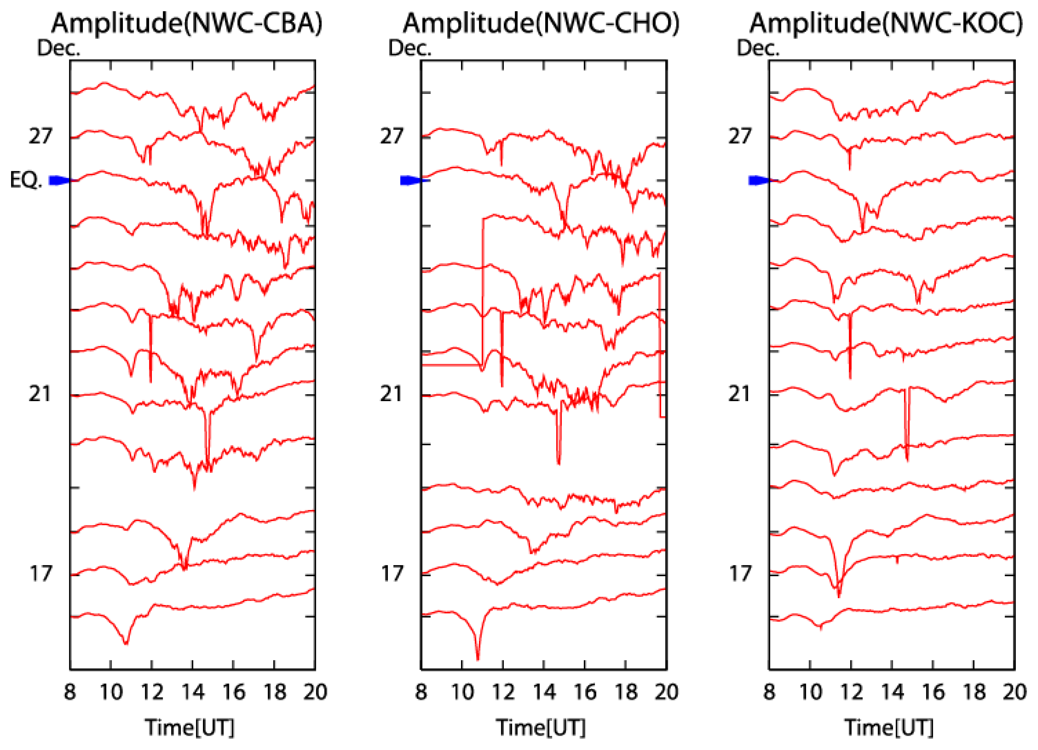
There have been proposed two methods of analysis to find the precursory effect of ionospheric perturbations as revealed from the VLF/LF data; (1) Terminator time method (Hayakawa et al., 1996; Molchanov and Hayakawa, 1998), and (2) Nighttime fluctuation analysis (Shvets et al., 2004a, b; Roznoi et al., 2004; Maekawa at al., 2006). As shown in Fig. 5, the propagation path is approximately in the N-S meridian plane, so that the terminator time method is not so effective for this path. Because the terminator time method is effective mainly for the E-W propagation direction (Maekawa and Hayakawa, 2006). Hence, we have adopted the fluctuation analysis. Fig. 6 is the sequential plot of nighttime amplitude of NWC signal observed at the three observing sites (Chiba (CBA), Chofu (CHO), and Kochi (KOC)). It is easy to understand qualitatively that there is an increased fluctuation in the nighttime amplitude at all the stations. Then, we will estimate this nighttime fluctuation quantitatively. We use the nighttime L.T. time internal for six hours (L.T. = 21 h to 03 h), and we estimate the difference dA(t) (≡ A(t) – <A(t)>) where A(t) is the VLF amplitude at the time t and <A(t)> is the average value over ±15 days (one month) at the same time t. Finally, we integrate dA2 over the relevant nighttime six hours, and we have one data for each day.
As is shown in Maekawa et al. (2006), we have shown the analysis result during the two years of 2004 and 2005. This long-term analysis was used to infer that the VLF nighttime fluctuation seems to be depleted during seismically quiet periods.
The fifth Fresnel zone shown in Fig. 5 is already found to be useful and effective as the VLF sensitive zone for earthquakes with magnitude 6.0-7.0 (Hayakawa et al., 1996; Molchanov and Hayakawa, 1998), when we think of the possible size of the seismo-ionospheric perturbations. This Sumatra earthquake is extremely huge (M = 9.3), so that we expect an extremely large area of ionospheric perturbations for this earthquake. By simply using either the formula on the preparation zone size by Dobrovolsky et al. (1979) or the empirical formula on the size of ionospheric perturbations by Ruzhin and Depueva (1996), the radius of preparation zone or possible ionospheric perturbation is estimated to be of the order of 7,000-8,000 km. The empirical formula by Ruzhin and Depueva (1996) is mainly based on the events mainly up to M = 7.0 or so, so that it is questionable for us to use this formula even up to M = 9.3. Even though, it may be reasonable to anticipate that the VLF propagation path from the transmitter, NWC to Japanese VLF sites is definitely influenced very much, or perturbed because the distance of the epicentre from the great-circle path is only 2,000 km.
As is already shown in Horie et al. (2007a), the geomagnetic activity just around the Sumatra earthquake (e.g. ±one month around the earthquake) is found to be relatively quiet except just after the middle of January, 2005 when the ΣKp exceeds 40 (disturbed). For example, in December, 2004, we have found relatively quiet geomagnetic activity. We look at the VLF fluctuations just before the Sumatra earthquake. It is very fortunate that we find very prolonged seismically quiet period before the Sumatra earthquake. Fig. 7 is the extended figure for the limited time period just around the earthquake time. But, you see now the temporal evolutions of the nighttime fluctuation (the same integrated dA2 over the night) at three stations (Chiba in black, Chofu in blue and Kochi in pink), together with the corresponding running value of m (mean) +2σ (standard deviation) over ±15 days (with the same color). We notice one sharp peak on 8 December, 2004 and a prolonged maximum during the period of December 21, 2004 to January 2, 2005. In the case of the fluctuation enhancement on 8 December, 2004, we notice a significant enhancement at Chiba (in black) exceeding (m + 2σ) line. However, the fluctuation at Chofu (in blue) is not found to exceed the (m + 2σ) line (given in the figure in pink) and also there is no enhancement at all at Kochi (in red). Taking into account these facts, we may conclude that the amplitude fluctuation is taking place significantly only at Chiba, which means that this enhancement on 8 December, 2004 might be the effect only for the NWC-Chiba path. Next we discuss the prolonged period of amplitude fluctuation during the period of December 21, 2004 to January 2, 2005. During this period we notice the simultaneous enhancement in fluctuations at the three observing sites (Chofu (in blue), Chiba (in black) and Kochi (in red)), which means that this prolonged fluctuation is global, and the NWC-Japan propagation path is strongly disturbed. The fluctuation at Chofu (in blue) is found to exceed significantly the (m + 2σ) line at Chofu a few days before the earthquake. Also, we recognize the similar and significant enhancement in Chiba and also in Kochi. You can notice the excess of the nighttime fluctuation over the corresponding (m + 2σ) line both at Chofu and Kochi. Even after the main shock (M = 9) on 26 December, 2004, there occurred several aftershocks on 1 ∼ 4 January, 2005 with magnitudes in a range from 6.1 to 6.7. In correspondence with this high seismic activity, there have been observed the prolonged VLF fluctuation during the period of 21 December, 2004 to 2 January, 2005.
When we look at the temporal evolutions in Fig. 6, we can easily identify clear wave-like structures in the data. Our visual inspection could give us an idea that there exist clear wave-like structures, for example, on 16, 24 and 26 December, 2004. These structures are quantitatively investigated by means of the wavelet and cross-correlation analyses. It is expected that these fine structures like wave-like structures could provide us with the information on how the ionosphere is perturbed in association with earthquakes.
We perform the wavelet analysis with a mother wavelet of the complex Morlet (Daubechies, 1990) to the difference dA(t) (Shvets et al., 2004a, b; Rozhnoi et al., 2004; Maekawa et al.,2006), and compute the spectral intensity of the VLF fluctuation dA. Next we quantitatively estimate the time delay between these 2 stations by using the cross-correlation method.
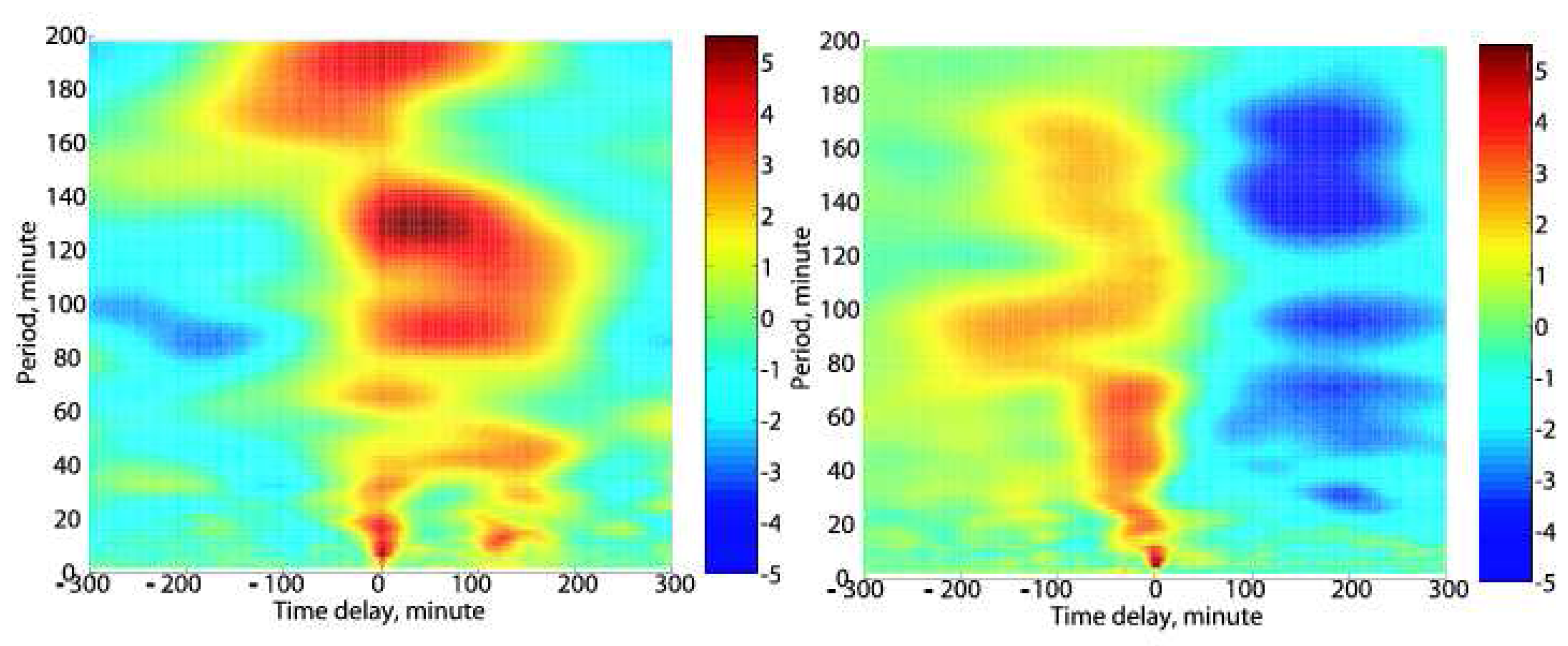
Fig. 8 is the summary of the cross-correlation analysis on the time delay of the Chiba data with respect to Kochi on the basis of superimposed epoch analysis. The left panel in Fig. 8 corresponds to the period of 16 December to 26 December, 2004 (that is, 11 days) before the earthquake. While, the right panel is the corresponding result for the period after the earthquake (2 May to 12 May, 2005) (i.e. quite period). An important point is that the fluctuations in amplitude (dA(t)) is very enhanced in the period of 20-100 minutes before the earthquake. This epoch analysis in the left panel indicates the clear presence of time delay or wave-like structure before the earthquake. The period of fluctuation is confirmed to range from 20-30 minutes to above 100 minutes, and the time delay at the Chiba is around 2 hours with respect to Kochi. There is no significant frequency dependence (dispersion) in the time delay. The right panel of Fig. 8 shows no such wave-like structures at all after the earthquake. So that, the presence of such wave-like structures is likely to be a precursory signature of this earthquake.
Before the earthquake, we could notice an enhancement in the fluctuation spectra in the frequency range from 20-30 minutes to about 100 minutes. This period corresponds to that of atmospheric gravity wave (AGW) (30 to 180 minutes) (Grossard and Hooke, 1975; Hooke, 1977) and this AGW is considered to be a possible and promising candidate for the lithosphere-ionosphere coupling (Molchanov et al., 2001; Miyaki et al., 2002; Shvets et al., 2004a, b). The wavelet at Chiba is delayed by about 2 hours with respect to that at Kochi, which is indicative of its propagating nature from the epicenter toward outsides. On the assumption that the wave is propagating radially from the epicenter, we can estimate the propagation distance between the NWC-KOC and NWC-CBA is estimated to be ∼ 150 km. So that we can estimate the wave propagation velocity of our wave-like fluctuation to be about 20 m/s. This value seems to be in good agreement with the theoretical estimation of AGWs (Kichengast, 1996; Hooke, 1968). The experimental evidence on the wave like fluctuations as a precursor to this Sumatra earthquake might be considered to be an evidence of the important role of AGW in the lithosphere-ionosphere coupling. Further details have appeared in Horie et al. (2007b).
The same NWC signals have been detected on board the French satellite, DEMETER, which has indicated that the signal to noise ratio (the ratio of the VLF signal to the background noise) is found to be significantly depressed during one month before the earthquake, and that the diameter of the ionospheric perturbation as seen on the satellite is about 5,000 km (Molchanov et al., 2006). This satellite finding on the presence of the ionospheric perturbation in association with the Sumatra earthquake and its spatial scale are found to be a further support to our ground-based VLF finding.
4. Lithosphere-ionosphere coupling mechanism
Even though it seems highly likely that the ionosphere is disturbed before an earthquake, it is poorly understood how the ionosphere is perturbed by the precursory seismic activity in the lithosphere. Hayakawa et al. (2004a, b) have already proposed a few possible hypotheses on the mechanism of coupling between the lithospheric activity and ionosphere; (1) chemical channel, (2) acoustic channel, and (3) electromagnetic channel. As for the first channel, the geochemical quantities (such as surface temperature, radon emanation etc.) induce the perturbation in the conductivity of the atmosphere, then leading to the ionospheric modification through the atmospheric electric field (e.g., Pulinets and Boyarchuk, 2004; Sorokin et al., 2006). The second channel is based on the key role of atmospheric oscillations in the lithosphere-atmosphere-ionosphere coupling, and the perturbation in the Earth's surface (such as temperature, pressure) in a seismo-active region excites the atmospheric oscillations traveling up to the ionosphere (Molchanov et al., 2001; Miyaki et al., 2002; Shvets et al., 2004a, b). The last mechanism is that the radio emissions (in any frequency range) generated in the lithosphere propagate up to the ionosphere, and modify the ionosphere there by heating and/or ionization. But this mechanism is found to be insufficient because of the weak intensity of lithospheric radio emissions (Molchanov et al., 1995). So, the 1st and 2nd mechanisms are likely candidates for this coupling(Molchanov and Hayakawa, 2007).
Our latest finding mentioned in the previous section is thought to provide evidence on the important role of AGWs in the lithosphere-atmosphere-ionosphere coupling. The observational evidence is, however, not much, so that we need to accumulate more facts on the generation mechanism. We can say the same thing for the 1st mechanism of chemical channel, and the subject, itself, is extremely interesting and challenging.
5. Concluding remarks
Short-term earthquake prediction is of essential importance for human beings in order to mitigate the earthquake disasters. The most promising candidate for this short-term earthquake prediction is recently recognized to be the monitoring of the ionosphere. We have proposed the VLF/LF radio sounding for seismo-ionospheric perturbations, and in this review paper we have presented a lot of convincing evidence on the presence of ionospheric perturbations associated with earthquakes on the basis of statistical and case studies. The most important point at the moment is the accumulation of convincing results as many as possible, which is being realized by this VLF/LF radio sounding with the characteristic nature of an integration observation.
We are sure about the presence of ionospheric perturbations associated with earthquakes, but more coordinated observations are highly required in order to elucidate the mechanism of lithosphere-atmosphere-ionosphere coupling as the final goal of seismo-electromagnetic studies. For example, we choose a test site where we carry out a highly coordinated measurement; different kinds of observations including surface monitoring, lithospheric radio emissions (e.g., ULF emissions), atmospheric effect (such as studied by over-horizon VHF signals) and ionospheric effect (as studied by subionospheric VLF/LF waves in this review).
Acknowledgments
The VLF/LF network was established within the framework of the Frontier Project by the former NASDA, to which we are grateful. Thanks are also due to NiCT (R and D promotion scheme funding international joint research) for its support. Finally, the author would like to thank Messrs S. Maekawa and T. Horie for their contribution.
References and Notes
- Biagi, P.F.; Piccolo, R.; Castellana, L.; Maggipinto, T.; Ermini, A.; Martellucci, S.; Bellecci, C.; Perna, G.; Capozzi, V.; Molchanov, O. A.; Hayakawa, M.; Ohta, K. VLF-LF radio signals collected at Bari (South Italy): a preliminary analysis on signal anomalies associated with earthquakes. Natural Hazards Earth System Sci. 2004, 4, 685–689. [Google Scholar]
- Cervone, G.; Maekawa, S.; Singh, R.P.; Hayakawa, M.; Kafatos, M.; Shvets, A. Surface latent heat flux and nighttime LF anomalies prior to the Mω = 8.3 Tokachi-Oki earthquake. Natural Hazards Earth System Sci. 2006, 6, 109–114. [Google Scholar]
- Daubechies, I. The wavelet transform time-frequency localization and signal analysis. IEEE Trans. Inform. Theory 1990, 36, 961–1004. [Google Scholar]
- Dobrovolsky, I. R.; Zubkov, S. I.; Myachkin, V. I. Estimation of the size of earthquake preparation zones. Pure and Applied Geophysics 1979, 117, 1025–1044. [Google Scholar]
- Gokhberg, M. B.; Gufeld, I. L.; Rozhnoy, A. A.; Marenko, V. F.; Yampolsky, V. S.; Ponomarev, E. A. Study of seismic influence on the ionosphere by super long wave probing of the Earth-ionosphere waveguide. Phys. Earth Planet. Inter. 1989, 57, 64–67. [Google Scholar]
- Grossard, E. E.; Hooke, W. H. Waves in the Atmosphere (Atmospheric Infrasound and Gravity Wave – Their Generation and Propagation); Elsevier Sci. Pub. Co.: Amsterdam, 1975. [Google Scholar]
- Gufeld, I. L.; Rozhnoi, A. A.; Tyumensev, S. N.; Sherstuk, S. V.; Yampolsky, V. S. Radiowave disturbances in period to Rudber and Rachinsk earthquakes. Phys. Solid Earth 1992, 28, 267–270. [Google Scholar]
- Hayakawa, M.; Molchanov, O. A.; Ondoh, T.; Kawai, E. The precursory signature effect of the Kobe earthquake on VLF subionospheric signals. J. Comm. Res. Lab , Tokyo 1996, 43, 169–180. [Google Scholar]
- Hayakawa, M. Atmospheric and Ionospheric Electromagnetic Phenomena Associated with Earthquakes; Terra Sci. Pub. Co.: Tokyo, 1999; p. 996. [Google Scholar]
- Hayakawa, M.; Molchanov, O. A. (Eds.) Seismo Electromagnetics: Lithosphere - Atmosphere -Ionosphere Coupling; TERRAPUB: Tokyo, 2002; p. 477.
- Hayakawa, M. Electromagnetic phenomena associated with earthquakes: A frontier in terrestrial electromagnetic noise environment. Recent Res. Devel. Geophysics 2004, 6, 81–112. [Google Scholar]
- Hayakawa, M.; Molchanov, O. A.; NASDA/UEC team. Summary report of NASDA's earthquake remote sensing frontier project. Phys. Chem. Earth 2004a, 29, 617–625. [Google Scholar]
- Hayakawa, M.; Molchanov, O. A. NASDA/UEC team. Achievements of NASDA's Earthquake Remote Sensing Frontier Project. Terr. Atmos. Ocean. Sci. 2004b, 15, 311–328. [Google Scholar]
- Hayakawa, M.; Ohta, K.; Maekawa, S.; Yamauchi, T.; Ida, Y.; Gotoh, T.; Yonaiguchi, N.; Sasaki, H.; Nakamura, T. Electromagnetic precursors to the 2004 Mid Niigata Prefecture earthquake. Phys. Chem. Earth 2006, 31, 356–364. [Google Scholar]
- Hooke, W. H. Ionospheric irregularities produced by internal atmospheric gravity waves. J. Atmos. Solar-terr. Phys. 1968, 30, 795–823. [Google Scholar]
- Hooke, W. H. Rossby-planetary waves, tides, and gravity waves in the upper atmosphere. In The Upper Atmosphere and Magnetosphere; Nat. Acad. Sci.: Washington, 1977; pp. 130–140. [Google Scholar]
- Horie, T.; Maekawa, S.; Yamauchi, T.; Hayakawa, M. A possible effect of ionospheric perturbations for the Sumatra earthquake, as revealed from subionospheric VLF propagation (NWA-Japan). Int'l J. Remote Sensing 2007a, 28, 3133–3139. [Google Scholar]
- Horie, T.; Yamauchi, T.; Yoshida, M.; Hayakawa, M. The wave-like structures of ionospheric perturbation associated with Sumatra earthquake of 26 December, 2004. J. Atmos. Solar-terr. Phys. 2007b, 69, 1021–1028. [Google Scholar]
- Kichengast, G. Elucidation of the physics of the gravity wave – TID relationship with the aid of theoretical simulations. J. Geophys. Res. 1996, 101, 13353–13368. [Google Scholar]
- Maekawa, S.; Hayakawa, M. A statistical study on the dependence of characteristics of VLF/LF terminator times on the propagation direction. Inst. Electr. Engrs. Japan, Fundamentals and Materials Special Issue on Recent Progress in Seismo-Electromagnetics. 2006, 126. [Google Scholar]
- Maekawa, S.; Horie, T.; Yamauchi, T.; Sawaya, T.; Ishikawa, M.; Hayakawa, M.; Sasaki, H. A statistical study on the effect of earthquakes on the ionosphere, based on the subionospheric LF propagation data in Japan. Ann. Geophysicae 2006, 24, 2219–2225. [Google Scholar]
- Miyaki, K.; Hayakawa, M.; Molchanov, O. A. The role of gravity waves in the lithosphere -ionosphere coupling, as revealed from the subionospheric LF propagation data. In Seismo Electromagnetics: Lithosphere - Atmosphere - Ionosphere Coupling; TERRAPUB: Tokyo, 2002; pp. 229–232. [Google Scholar]
- Molchanov, O. A.; Hayakawa, M.; Rafalsky, V. A. Penetration characteristics of electromagnetic emissions from an underground seismic source into the atmosphere, ionosphere, and magnetosphere. J. Geophys. Res. 1995, 100, 1691–1712. [Google Scholar]
- Molchanov, O. A.; Hayakawa, M.; Ondoh, T.; Kawai, E. Precursory effects in the subionospheric VLF signals for the Kobe earthquake. Phys. Earth Planet. Inter. 1998, 105, 239–248. [Google Scholar]
- Molchanov, O. A.; Hayakawa, M. Subionospheric VLF signal perturbations possibly related to earthquakes. J. Geophys. Res. 1998, 103, 17,489–17,504. [Google Scholar]
- Molchanov, O. A.; Hayakawa, M.; Miyaki, K. VLF/LF sounding of the lower ionosphere to study the role of atmospheric oscillations in the lithosphere-ionosphere coupling. Adv. Polar Upper Atmos. Res. 2001, 15, 146–158. [Google Scholar]
- Molchanov, O. A.; Rozhnoi, A.; Solovieva, M.; Akentieva, O.; Berthelier, J. J.; Parrot, M.; Lefeuvre, F.; Biagi, P. F.; Castellana, L.; Hayakawa, M. Global diagnostics of the ionospheric perturbations related to the seismic activity using the VLF radio signals collected on the DEMETER satellite. Natural Hazards Earth System Sci. 2006, 6, 745–753. [Google Scholar]
- Molchanov, O. A.; Hayakawa, M. Seismo-electromagnetics and Related Phenomena: History and Lates Results; TERRAPUB: Tokyo, 2007; in press. [Google Scholar]
- Ohta, K.; Makita, K.; Hayakawa, M. On the association of anomalies in subionospheric VLF propagation at Kasugai with earthquakes in the Tokai area, Japan. J. Atmos. Electr. 2000, 20, 85–90. [Google Scholar]
- Pulinets, S.; Boyarchuk, K. Ionospheric Precursors of Earthquakes; Springer: Berlin, 2004; p. 315. [Google Scholar]
- Rodgers, C.; McCormick, R. J. Remote sensing of the upper atmosphere by VLF. In Sprites, Elves and Intense Lightning Discharges; Füllekrug, M., et al., Eds.; Springer, 2006; pp. 167–190. [Google Scholar]
- Rozhnoi, A.; Solovieva, M. S.; Molchanov, O. A.; Hayakawa, M. Middle latitude LF (40 kHz) phase variations associated with earthquakes for quiet and disturbed geomagnetic conditions. Phys. Chem. Earth 2004, 29, 589–598. [Google Scholar]
- Ruzhin, Yu. Y.; Depueva, A. Kh. Seismoprecursors in space as plasma and wave anomalies. J. Atmos. Electr. 1996, 16, 271–288. [Google Scholar]
- Shvets, A. V.; Hayakawa, M.; Molchanov, O. A. Subionospheric VLF monitoring for earthquake-related ionospheric perturbations. J. Atmos. Electr. 2002, 22, 87–99. [Google Scholar]
- Shvets, A. V.; Hayakawa, M.; Maekawa, S. Results of subionospheric radio LF monitoring prior to the Tokachi (m = 8, Hokkaido, 25 September 2003) earthquake. Natural Hazards Earth System Sci. 2004a, 4, 647–653. [Google Scholar]
- Shvets, A. V.; Hayakawa, M.; Molchanov, O. A.; Ando, Y. A study of ionospheric response to regional seismic activity by VLF radio sounding. Phys. Chem. Earth 2004b, 29, 627–637. [Google Scholar]
- Sorokin, V. M.; Yaschenko, A. K.; Chmyrev, V. M.; Hayakawa, M. DC electric field formation in the mid-latitude ionosphere over typhoon and earthquake regions. Phys. Chem. Earth 2006, 31, 454–461. [Google Scholar]
- Yamauchi, T.; Maekawa, S.; Horie, T.; Hayakawa, M.; Soloviev, O. Subionospheric VLF/LF monitoring of ionospheric perturbations for the 2004 Mid-Niigata earthquake an their structure and dynamics. J. Atmos. Solar-terr. Phys. 2007, 69, 793–802. [Google Scholar]
Figure 1.
(a) Relative location of the VLF transmitter (Omega, Tsushima), our observatory at Inubo and the earthquake epicenter (x). The first Fresnel zone is indicated. (b) The sequential plot of diurnal variation (phase) (nearly the same pattern as for amplitude; and please pay attention to the variation in tm (morning terminator time) and te (evening terminator time). The shaded areas indicate the shift from the monthly mean value.
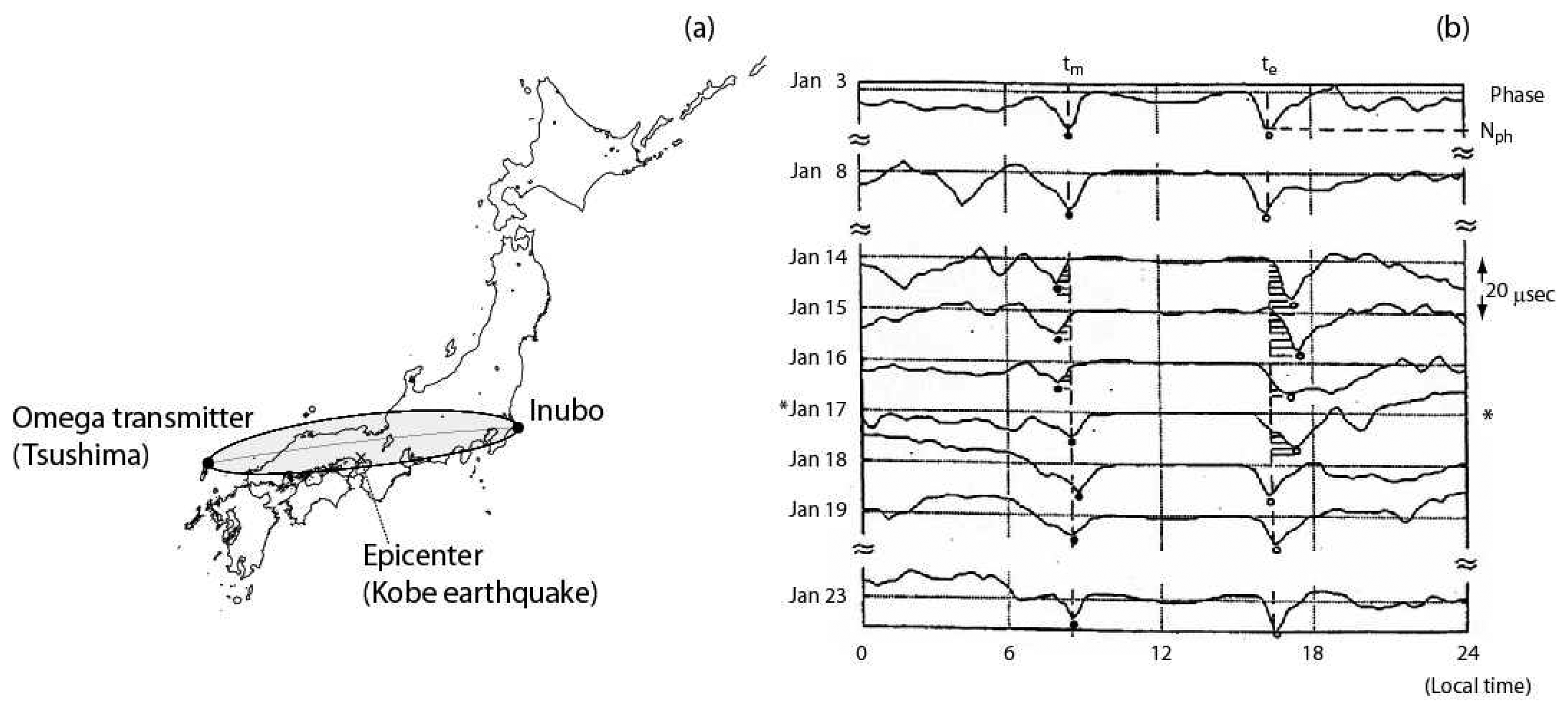
Figure 2.
VLF/LF network in Japan. Several observing stations (Moshiri (abbreviated as MSR), Chofu (CHO), Chiba (CBA), Shimizu (SMZ), Kasugai (KSG), Maizuru (MZR), and Kochi (KOC)) and several VLF/LF transmitter signals detected at each station. The situation for one station (MSR) is indicated, and receiving transmitters are JJY, NWC, JJI, NPM and NLK.

Figure 3.
Relative location of the LF transmitter, JJY in Fukushima and an observing station, Kochi. The sensitive area for this LF propagation path is also indicated; the circles with radius of 200km around the transmitter and receiver and by connecting the outer edges of these two circles. Also 92 earthquakes with conventional magnitude (M) greater than 5.0 are plotted, which took place within the sensitive area.

Figure 4.
Statistical test result for the amplitude (a) and dispersion (b). The day on the abscissa is defined as follows: day zero indicates the day of the earthquake, and minus (plus) means that the phenomenon takes place before (after) the earthquake. The important 2σ (σ: standard deviation) lines are plotted for the statistical test.
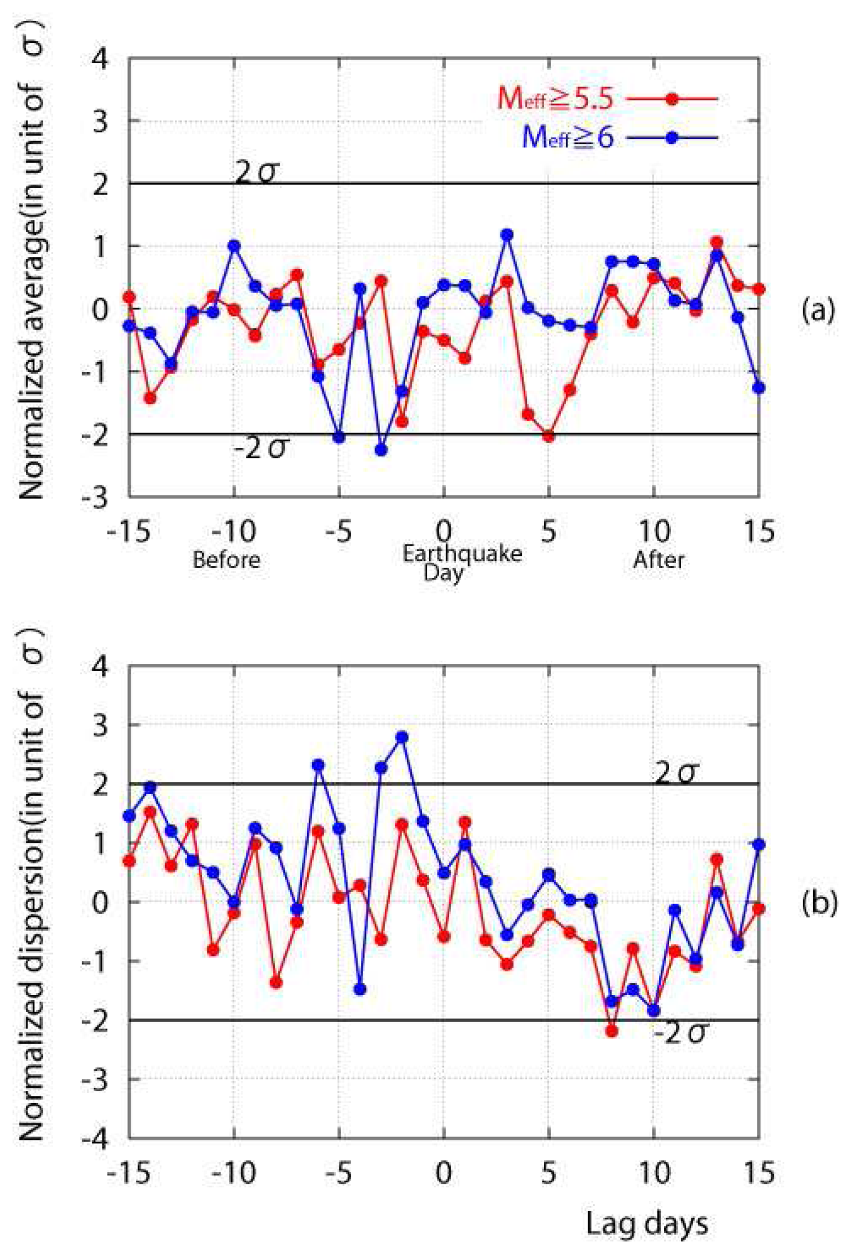
Figure 5.
Propagation paths from the transmitter, NWC (in Australia) to the two receiving sites (Kochi and Chofu). The fifth Fresnel zone for each propagation path is indicated. The earthquakes with magnitude greater than 6.0 within and just close to the VLF sensitive zone during the years of 2004 and 2005 are all indicated. The center of each circle corresponds to the earthquake epicenter, and the size of the circle indicates the earthquake magnitude. The color of earthquakes during the period of November, 2004 to May, 2005 indicates the earthquake depth. The date of the earthquake is indicated beside the circle (i.e. 4/10 means April 10). The Sumatra earthquake is far away from the great-circle paths, but it is indicated (12/26).
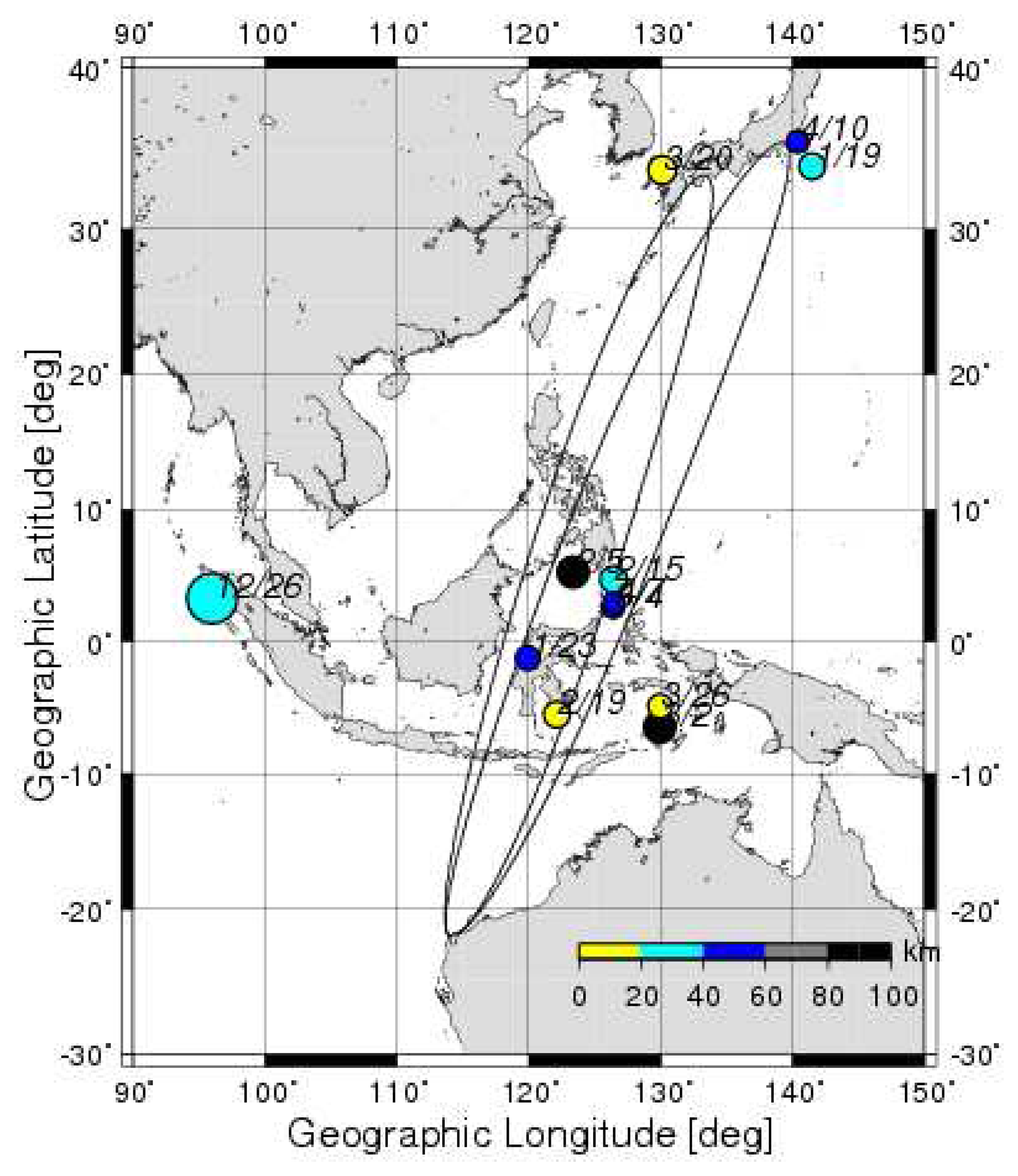
Figure 6.
Sequential plot of nighttime amplitude data of the NWC signal as observed at three Japanese observing stations (from left to right: CBA, CHO and KOC). Date goes from the bottom to the top, and the earthquake date is given by EQ. Time is given in UT, so that the Japanese local time (LT) is given by UT + 9 h.

Figure 7.
Temporal evolution of VLF amplitude nighttime fluctuation (dA2) at the three observing stations (Chofu (Blue), Chiba (Black), and Kochi (Red)). The red line indicates (m (mean)+2σ (σ: standard deviation)) at Chofu, and the corresponding lines refer to Chiba and Kochi. The earthquake with magnitude greater than 6.0 is plotted downward, and the earthquakes during the restricted period of November, 2004 to May, 2005 are characterized by different colors (color indicates the depth).
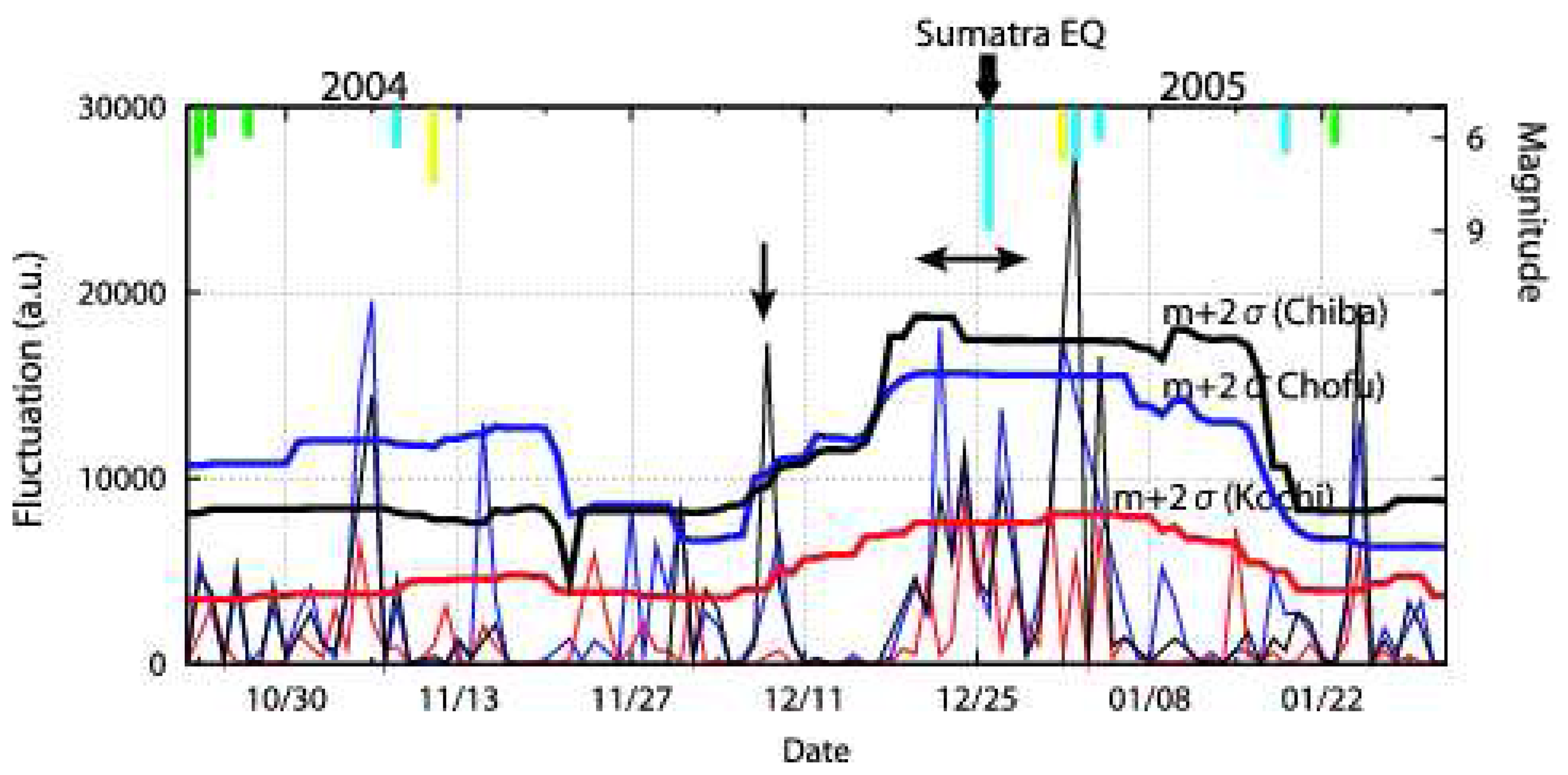
Figure 8.
The superimposed epoch analysis for the cross-correlation of fluctuation at the two stations of Chiba and Kochi. The left panel refers to the period before the earthquake (December 16 to December 26, 2004), while the right, a quite period after the earthquake (May 2 to May 12, 2005). The time delay at CBA on the abscissa is defined with respect to KOC (the delay of +2 hours in the left panel at CBA, means that the wave structure arrives at CBA 2 hours later with respect to KOC).
© 2007 by MDPI ( http://www.mdpi.org). Reproduction is permitted for noncommercial purposes.
Share and Cite
MDPI and ACS Style
Hayakawa, M. VLF/LF Radio Sounding of Ionospheric Perturbations Associated with Earthquakes. Sensors 2007, 7, 1141-1158. https://doi.org/10.3390/s7071141
AMA Style
Hayakawa M. VLF/LF Radio Sounding of Ionospheric Perturbations Associated with Earthquakes. Sensors. 2007; 7(7):1141-1158. https://doi.org/10.3390/s7071141
Chicago/Turabian StyleHayakawa, Masashi. 2007. "VLF/LF Radio Sounding of Ionospheric Perturbations Associated with Earthquakes" Sensors 7, no. 7: 1141-1158. https://doi.org/10.3390/s7071141