Asymptotic Effectiveness of the Event-Based Sampling According to the Integral Criterion

AGH University of Science and Technology, Department of Electronics, al. Mickiewicza 30, 30-059 Kraków, Poland
Sensors 2007, 7(1), 16-37; https://doi.org/10.3390/s7010016
Submission received: 10 August 2006
/
Accepted: 5 January 2007
/
Published: 6 January 2007
(This article belongs to the Special Issue Intelligent Sensors)
Abstract
:A rapid progress in intelligent sensing technology creates new interest in a development of analysis and design of non-conventional sampling schemes. The investigation of the event-based sampling according to the integral criterion is presented in this paper. The investigated sampling scheme is an extension of the pure linear send-on-delta/level-crossing algorithm utilized for reporting the state of objects monitored by intelligent sensors. The motivation of using the event-based integral sampling is outlined. The related works in adaptive sampling are summarized. The analytical closed-form formulas for the evaluation of the mean rate of event-based traffic, and the asymptotic integral sampling effectiveness, are derived. The simulation results verifying the analytical formulas are reported. The effectiveness of the integral sampling is compared with the related linear send-on-delta/level-crossing scheme. The calculation of the asymptotic effectiveness for common signals, which model the state evolution of dynamic systems in time, is exemplified.
1. Introduction
Intelligent sensors are sophisticated sensing devices possessing advanced functionality in terms of information processing, reliability, data fusion and integration. The intelligent sensor is essentially an event-based system intended to detect specified events of interest in a sensor field. Therefore, information from intelligent sensors is usually representative of a large class of system observations which are categorized as irregular observations [1]. Even if sensor reports are transmitted periodically, they may not appear to be periodic at the destination due to time-varying delivery delays or transmission errors handling in various network protocols. Moreover, in general the state of the objects being monitored evolves irregularly in time. To avoid a loss of valuable information between sampling instants, the sampling frequency in periodic reporting has to be set on a basis of predicting the worst-case signal changeability. However, setting a sampling rate by taking into account the worst-case conditions in a state variation is more or less wasteful since numerous useless samples are taken. Actually, many signals in sensory applications (e.g. temperature sensors, speech signals, electrocardiograms, etc.) show bursty statistical properties, i.e. these signals are constant for most of the time and may vary significantly only during short time intervals.
The irregular observations are defined to be message-based observations with possibly infrequent and non-periodic measurements, where the message indicates the source and the destination(s), the timestamp of a sample, the range of possible measurement values, and the protocol service specification (e.g. message service type, optional authentication, or network traffic prediction) [1]. For example, LonWorks/EIA-709 technology, that is widely used for the interconnection of intelligent sensor/actuator devices, provides programming objects called the Standard Network Variable Types (SNVT) specifying, by the convention, various common physical magnitudes (voltage, temperature, etc.), their range, unit, and resolution [2].
A special class of irregular observations is constituted by the event-based sampling schemes. This class is characterized by the functional relationship between the sampling instants and signal behavior. Thus, the event-based sampling is signal-dependent whereas the irregular sampling encompasses also signal-independent schemes. In the event-based sampling, the signal is sampled when the significant event occurs (i.e. a significant change of its state is noted) [13].
The most natural signal-dependent sampling strategy is the send-on-delta algorithm [3-6], known also as the level-crossing sampling [7,8] or deadbands concept [9]. Send-on-delta reporting is used, among others, by intelligent sensor nodes in LonWorks networked control systems [10]. According to the send-on-delta strategy, the sensor node does not broadcast a new message if the input signal remains within a certain interval of confidence. The hardware designs of level-crossing samplers equipped with the low-power asynchronous analog-to-digital converters are discussed in [7,8]. Such converters are not controlled by any global clock, but are enslaved by the analog input signal. Furthermore, the time intervals between consecutive amplitude-related events are quantized instead of the signal amplitude [8]. The asynchronous analog-to-digital converters establish a new research area especially attractive for wireless sensor technology.
Although the methods of analysis and design for periodically sampled systems is mature, the event-based systems theory is, as Aström and Bernhardsson pointed out, “still in its infancy” [6] with relatively few works studying several aspects of event-based functionality, see e.g. [5,6,9-13].
Generalizing the send-on-delta/level-crossing concept, the event-based strategy allows one to sample in a domain of various signal measures. The special classes are what is known as conventional uniform sampling in a time domain (periodic sampling) and uniform sampling in a value domain (level-crossing sampling/send-on-delta). However, by the appropriate definition of triggers (i.e. events that trigger sampling), the concept of the event-based sampling might be extended to advanced signal parameters [14]. From the practical point of view, the most important signal measures are such that have a significant physical interpretation (e.g. the integral, energy, etc). Using these measures for the trigger definition, the integral sampling, and the sampling in the energy domain respectively, might be constituted.
The paper discusses an event-driven strategy, where the input signal is sampled according to the integral criterion. A use of the integral criterion for triggering sampling operations has been known in control system technology since the early 60s at least [16]. Nowadays, the rapid progress in intelligent sensing technology creates new interest in a development of analysis and design of non-conventional sampling schemes. The main motivation to use the integral sampling is that the performance of the monitoring or control system is usually defined as the integral of the absolute value of the error (IAE) [9]. The sampling according to the integral criterion may be treated as an extension of the linear send-on-delta strategy, and called the integral send-on-delta concept.
It is intuitively comprehensible that a use of the signal-dependent sampling instead of conventional periodic updates reduces the mean rate of messages generated by a sensor node since sampling occurs when “it is required”. For example, a use of the adaptive sampling scheme approximating the integral criterion, and proposed by Dorf et al. in the early 60s, yields from 20% to 50% of the savings in the number of samples over a long period of time [16]. However, no explicit formula has been derived to evaluate how much effective it is in a general case. To the author's knowledge, the precise evaluation of the integral event-based sampling effectiveness has not been addressed in the scientific literature until now. The present paper shows that the asymptotic effectiveness might be easily estimated for a given sampled signal using the closed-form analytical formula.
The paper contribution consists of:
- -
- the analytical approximation of mean rate of the event-based sampling according to the integral criterion,
- -
- the formulation and the analytical proof of the theorem that evaluates the asymptotic effectiveness of the integral sampling,
- -
- the observation that the asymptotic effectiveness is a measure embedded in the sampled signal that does not depend on the sampling resolution,
- -
- the simulative validation of the analytical results,
- -
- the applications of the derived formula for common signals in dynamic systems (i.e. derivation of explicit formulas and numerical solutions for the typical transient responses),
- -
- the comparison of the effectiveness of the integral sampling to the effectiveness of the send-on-delta/level-crossing sampling.
2. Event-based sampling according to the integral criterion
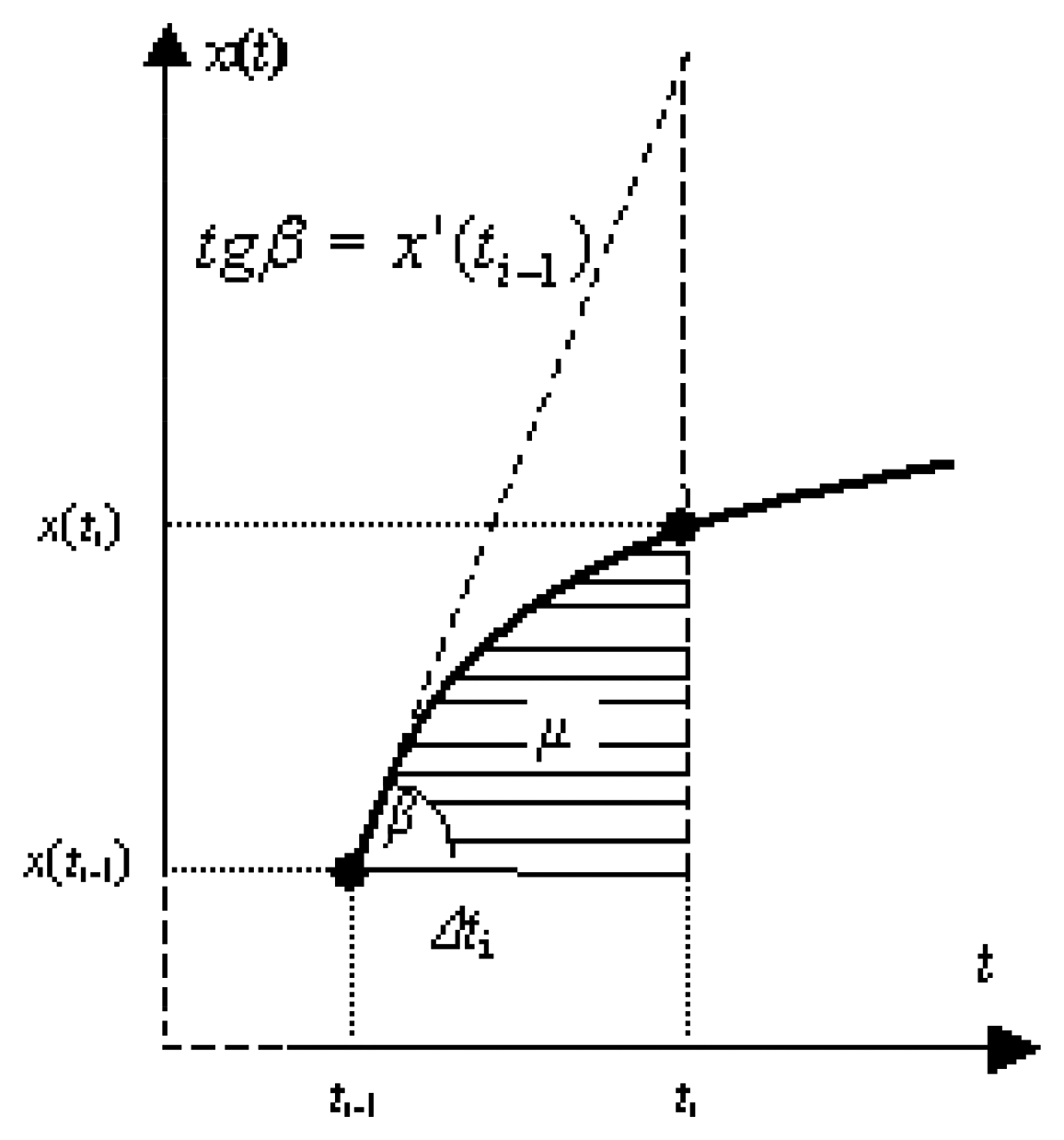
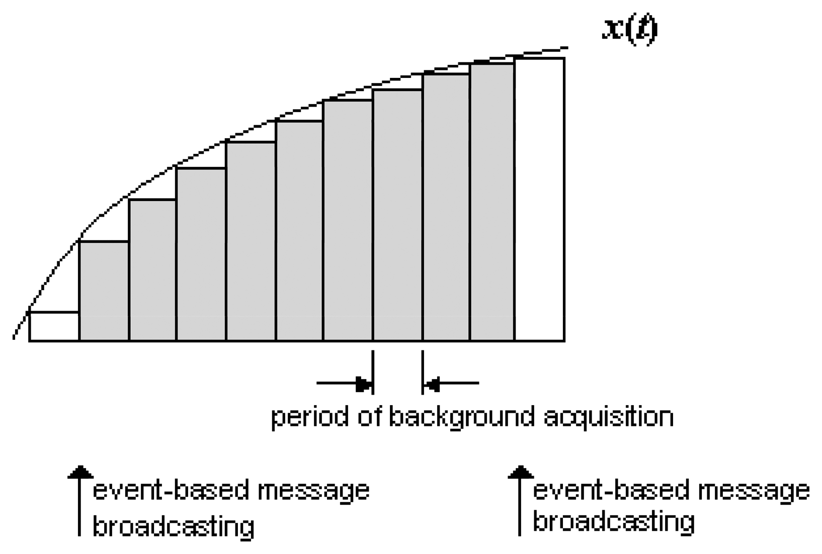
By the definition, a signal x(t) is sampled according to the uniform integral criterion if the integral of the absolute error (IAE) (i.e. the integral of the absolute difference between the current signal value x(t), and the value included in the most recent sample x(ti−1)), accumulated over the ith sampling interval (tt−1, ti), reaches a certain constant threshold μ>0 (Fig. 1):
where i = 1,2, …,n is the index of samples taken during the analyzed time interval [a,b].
We assume also that the zero-order hold is used to keep the value of the most recent sample between sampling instants.
2.1. Motivation of use of the integral sampling
There are a few reasons to use the event-based integral criterion in monitoring and control systems.
First of all, integral sampling as the event-based scheme is efficient for sampling burst signals. The integral criterion shows some inherent advantages. In particular, the integral sampling is beneficial to applications where a critical problem of sampling process is the accuracy of approximation of a continuous-time signal by a sequence of discrete-time samples. The integrated absolute sampling error is a more useful measure of the signal tracking quality than a pure linear error that constitutes the level-crossing scheme. It is because the former is a non-decreasing function of time (see (1)) unlike the latter. As a result, the positive and the negative errors do not compensate each other in the integral absolute sampling scheme.
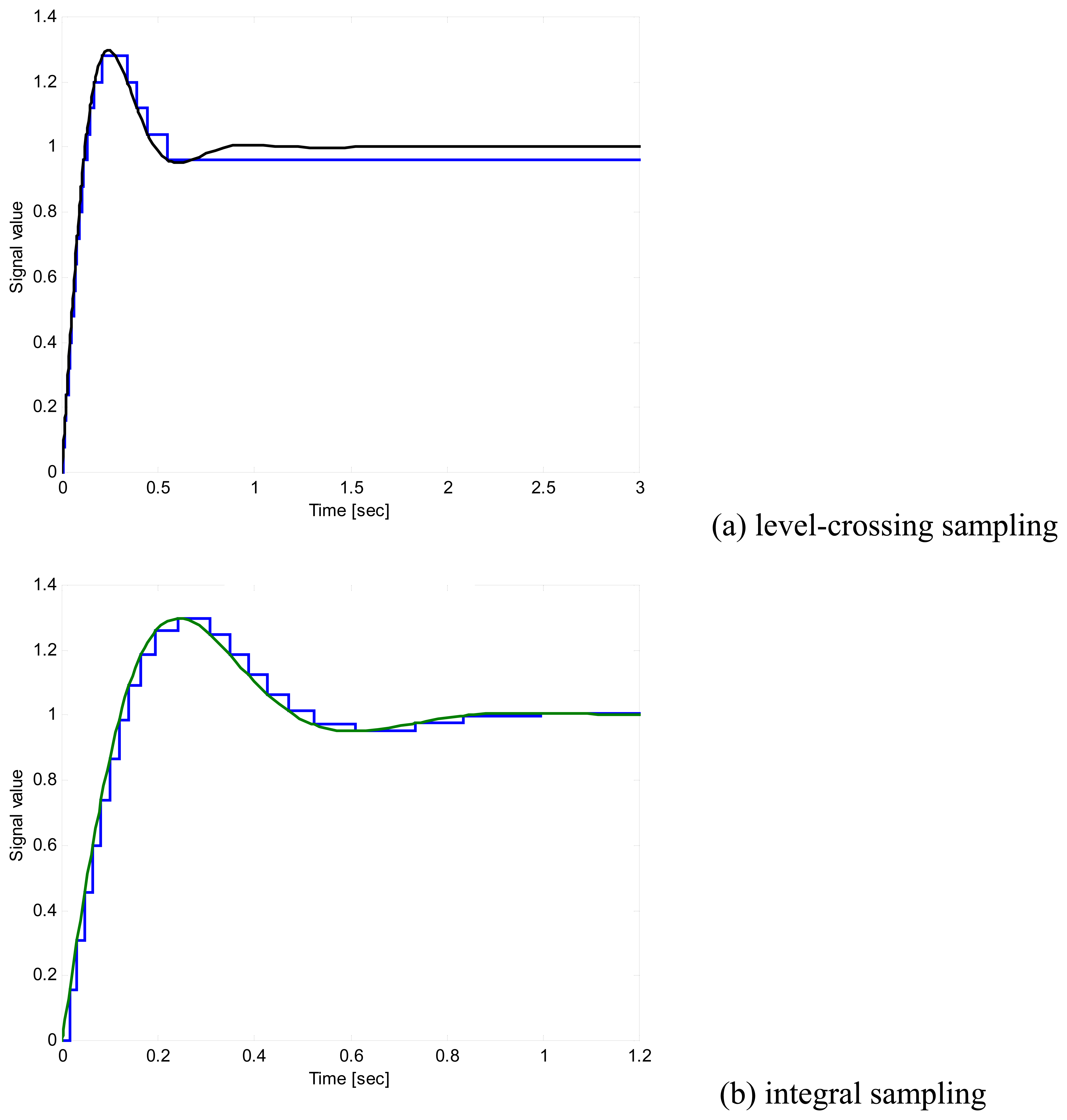
By the definition, the level-crossing sampling is triggered if a temporary deviation of a signal appears. Instead, in the integral sampling, a summation of the absolute temporal sampling errors is taken into account. Let us consider, as an example, a control system where the controlled variable reaches its equilibrium state and becomes nearly constant (Fig. 2). In the level-crossing scheme, sampling sometimes may not be triggered during a long time since the signal changes are not large enough to activate the next sampling operation (Fig. 2a). If the integral criterion is used instead, the integrated error accumulated in time triggers next sampling operations, and the signal tracking becomes more accurate (Fig. 2b). Moreover, as it was mentioned, the performance of the monitoring and control system is usually defined as the integral of the absolute value of the error (IAE) [9], which directly corresponds to the definition of the integral sampling criterion.
Finally, the event-based integral criterion is useful in case of indirect measurements, in particular if the measurements in the domain of the absolute primitive function are carried out (e.g. if the electric charge is measured by the sampling of the current intensity signal or if the covered distance is estimated on the basis of tracking the velocity). In order to detect the uniform changes of the indirect variable (the charge, or the position), the measured signal (the current intensity, or the velocity, respectively) has to be sampled in the absolute primitive function domain. The example of signal sampling using the event-based integral criterion with the zero-order hold is presented in Fig. 2b.
2.2. Trigger detection
A detection of triggers (i.e. events that cause the sampling operation) in the integral sampling can be accomplished using pure analog circuitry. An alternative solution is the use of the compound architecture for data acquisition where the continuous-time signal is first periodically oversampled. Next, on the top of the time-triggered acquisition, the event-triggered communication and processing activities are implemented, i.e. a detection of a trigger over a set of periodic samples is provided (Fig. 3) [17,18]. In other words, the periodic oversampling is followed by the low resolution difference quantificator. Such a compound approach, where the asynchronous events are presynchronized by background periodic sampling, is called the “upward” event-driven architecture [17,18].
3. Related works
The motivation of the development of effective sampling schemes is expressed by a fundamental question concerning the conversion of the physical reality into a set of discrete-time values: How the sampling points are to be selected in such a way that the discrete approximation of a continuous-time signal is as accurate as possible on the one hand, and the number of samples is minimized on the other?
3.1. Adaptive sampling
The idea of varying the sampling period and adjusting it to the current signal behavior has been investigated since the late 50s [4,16,19-25]. Various non-conventional sampling schemes have been proposed, among others, the adaptive sampling, which is a class of signal-dependent techniques closely related to the event-based schemes [16,19-25].
The adaptive sampling schemes are based on the real-time adjustment of the temporary sampling period to the predicted signal changes. The sampling period is allowed to vary from interval to interval in order to reduce the number of samples without degradation of the system response. The signal tracking performance in the adaptive sampling depends on the quality of the state estimation, i.e. the prediction of the signal behavior in the near future based on the knowledge of the signal in the past. The prediction takes advantage of a signal approximation by the truncated Taylor series over the sampling interval at the instant when the most recent sample has been taken. The maximum sampling period Tmax is bounded arbitrary and dictated by several factors such as communication bandwidth, reliability [13], stability of the closed-loop control system [16], or the performance of particular applications. The essential difference between the adaptive sampling and the event-based one is that the former is based on the time-triggered strategy where the sampling instants are controlled by the timer, and the latter belongs to the event-triggered systems where the sampling operations are determined only by signal amplitude variations rather than by the progression of time.
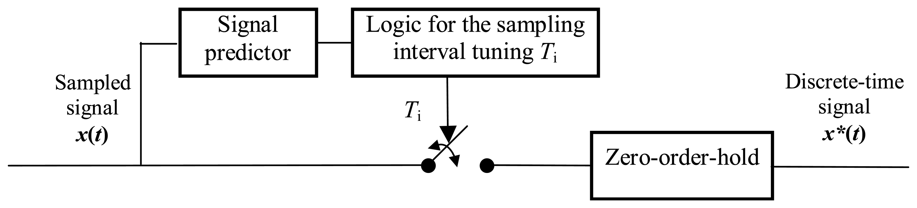
A model of the adaptive sampling system is depicted in Fig. 4. Most of the adaptive sampling algorithms have been derived heuristically [16,19,20]. In particular, Dorf et al. proposed the constant integral-difference sampling law [16] which corresponds to the integral criterion analyzed in the present paper, and Mitchell et al. introduced the constant absolute-difference criterion that is the (adaptive sampling) equivalent of the pure (event-based) level-crossing/send-on-delta algorithm [19]. The aim of the adaptive sampling system design is to derive an explicit expression for the sampling interval length basing on the assumed criterion.
The integral criterion proposed by Dorf et al. is the closest to the scope of the present study although the former belongs to adaptive sampling schemes, and the latter is the event-based one. The explicit expression for the evaluation of varying sampling interval Ti according to Dorf's integral-difference adaptive sampling law is
, where C = const depending on the assumed sampling resolution, and |x′(ti−1)| is the absolute value of the signal time derivative at the instant ti−1 when the most recent sample has been triggered [16]. Thus, the implementation of the adaptive sampling laws requires the real-time evaluation of the absolute signal derivative |x′(t)|. Since the implementation of a sampling law definded by the above formula for Ti was too compex in the early 60s, Dorf et al. proposed the linear approximation of this formula. Additionally, both the lower and the upper bounds on the sampling interval Ti are introduced to the sampling law arbitrary. The authors provided some numerical results showing that this approximated criterion yields from 20% to 50% of the savings in the number of samples over a long period of time comparing to the conventional periodic sampling [16]. However, no explicit formula has been derived to evaluate how much effective it is in a general case.
Next, Hsia has noticed that both Dorf s and Mitchel's heuristic adaptive sampling criteria might be derived from the same integral-difference criterion of different thresholds, and proposed a unified approach to a design of adaptive sampling laws [21]. In subsequent works the propositions of generalized criteria for adaptive sampling have been introduced [22,25]. These criteria combine a sampling resolution with a sample cost modelled by the proposed cost functions.
However, as follows from our experience, the adaptive sampling scheme has the significant disadvantage, which we call the “local extremum trap”. Namely, the estimated current sampling interval is theoretically infinite, although practically bounded to its maximum value Tmax, if the most recent sample is taken when the signal reached its local minimum or maximum (Fig. 5a). It is because the signal first time-derivative crosses zero at that moment and the predicted signal change is very low or even zero. As a result, the adaptive sampling is prone to the temporary instability of the signal tracking error (see Fig. 5a). On the other hand, the event-based integral sampling is in general not subject to similar problem since the (integral) sampling error is the same by the definition in every sampling interval (Fig. 5b).
Although the adaptive sampling has not been commonly applied in practice, there are selected application areas where it has been successfully utilized (see the overview of adaptive sampling applications in [24]). Furthermore, the adaptive sampling in control systems is nowadays still an active research topic, e.g. see [23].
3.2. Event-based sampling versus pulse frequency modulation (PFM)
There are some existing systems based on the same philosophy as the event-based sampled-data systems. In particular, the pulse frequency modulation (PFM) belongs to the class of level-crossing sampling systems, and the integral pulse frequency modulation (IPFM) corresponds to the event-based sampling according to the integral criterion [24,26]. The operation of the IPFM is summarized as follows. First, the input signal is integrated. Next, when the signal on the integrator output reaches the fixed reference value, a pulse is generated, the integrator is reset, and the cycle starts again. Thus, the signal on the IPFM modulator output consists of a series of pulses. The IPFM is widely utilized in biomedical applications for the estimation of the cardiac event series and the heart rate variability (HRV) [27].
4. Analysis of the event-based integral sampling
In this section, a derivation of the analytical formulas for the uniform event-based sampling according to the integral criterion is presented.
4.1 Sampled signal definition
We assume that a sampled signal is any time-varying quantity. Our discussion is restricted to a class of signals that are samplable (i.e. the signals of bounded variation) such that the sampling error can be controlled by tuning the sampling interval.
The definition of a function of bounded variation was introduced by C. Jordan in 1881 [28]. We adopt it for signals as follows.
Definition 1
A signal x(t) defined over a time interval [a,b] is said to be of bounded variation if the following sum is bounded:
for every partition of the interval [a,b] into subintervals (tj−1, t j), where j = 1,2,…,k; and t0 = a, tk = b. The measure denoted by and defined as:
is said to be a total variation of a signal x(t) on the interval [a,b].
A signal of bounded variation is not necessarily continuous, but is differentiable almost everywhere. Moreover, x(t) can have discontinuities of the finite-jump type at most [29,30]. If x(t) is continuous, the total variation
might be interpreted as the vertical component (ordinate) of the arc-length of the x(t) graph, or alternatively, as the sum of all consecutive peak-to-valley differences.
All the signals which appear in the physical reality or are generated in the laboratory can be approximated by a class of signals of bounded variations.
In the context of linear time-invariant (LTI) system with a transfer function H(s), the total variation of the step response s(t) is the peak gain of a system (defined as the largest ratio of the L∞ norm of the output to the L∞ norm of the intput) [31,32]:
This observation appears firstly in [31]. On the other hand, it can be shown that the peak gain of a transfer function is equal to the L1 norm of its impulse response [32]:
Therefore, on a basis of (2b) and (2c), the total variation of LTI system step response might be interpreted as the integrated absolute area (L1 norm) of the corresponding impulse response h(t) [33]:
4.2. Integral sampling resolution
The next definition specifies a metric that describes the sampling accuracy characterized by the integral absolute error (IAE) (see Fig. 1). We will use it in the subsequent sections for the comparison of sampling schemes.
Definition 2
If the integral absolute sampling error (IAE) is used for the evaluation of the sampling accuracy, the resolution v of the sampling scheme over a time interval [a, b] is defined as the inverse of the maximum δ of the set of numbers δi, i.e.:
where, and
is IAE accumulated over the ith sampling interval (ti−1,ti) ⊂ [a,b].
As follows from Definition 2, we assume that the sampling resolution is defined just by the worst-case (maximum) integral absolute sampling error (IAEmax), i.e. δ = max{δi}. In the uniform event-based sampling according to the integral criterion, IAE is the same in every sampling interval (i.e. δi = δ = μ, see (1)), thus the sampling resolution equals v = 1/μ. On the other hand, in the periodic sampling, IAE varies among the sampling periods and reaches its maximum IAEmax only during the fastest changes of the sampled signal.
4.3. Mean and maximum sampling rate
Let x(t) be a signal of bounded variation over the time interval [a,b].
Theorem 1
The mean sampling rate m in the integral event-based sampling scheme for a sampling resolution v = 1/μ is approximated by the following formula:
where is the mean of the square root of the signal derivative absolute value defined as follows:
Proof
By letting the signal x(t) be approximated by a truncated Taylor series, if the threshold μ is small enough:
we have:
where x′ (ti−1) is the signal time-derivative at the instant ti−1.
Taking into account (7), the criterion (1) can be approximately written as:
where Δti = ti−ti−1 is the length of the ith sampling interval.
Then, by the definition the mean length
of the sampling interval calculated for a number of n sampling intervals:
The mean sampling rate m (i.e. the average number of samples in a time unit) is given as follows:
For simplicity but without loss of generality, assume that t0= a, tn =b.
If we also assume that during each sampling interval Δti, i = 1, …, n, the signal derivative does not change significantly, (i.e. x′(t) ≅ const, t ∈ (ti−1,ti)), then:
On the basis of (9) we can write:
If the lengths of the sampling intervals Δti, i = 1,…,n are small enough, the sum of integrals on the right side of (15) can be approximated by the single integral taken over the whole time interval [t0,tn] ≡ [a,b]:
Thus, the proof has been completed.
Summing up, the mean sampling rate in the uniform event-driven integral sampling is expressed by two factors:
- -
- the mean of the square root of the signal derivative absolute value , which is a measure of the sampled signal x(t),
- -
- the resolution v = 1/μ of the integral event-based sampling.
On a basis of (12) we can also find the maximum sampling rate, which occurs during the fastest signal changes:
or respectively, the minimum intersample spacing:
where |x′(t)|max is the maximum of the absolute value of the first signal derivative with respect to the time during an interval [a,b]. The relationship (18) can be also derived directly from (9).
Thus, the maximum sampling rate is bounded implicitly by the threshold μ and the gradient |x′(t)| max of the signal derivative absolute value (i.e. the maximum slope of the sampled signal).
4.4. Integral sampling effectiveness
In order to estimate how effective the integral sampling is in terms of the sampling rate, we compare it with the conventional periodic observations assuming that both schemes have the same sampling resolution.
Definition 3
The effectiveness q of the event-based sampling according to the integral criterion (1) in a certain time interval [a,b] is defined as the ratio of the sampling frequency in the periodic scheme mT and the mean rate of samples m in the corresponding event-based scheme:
assuming that the sampling resolution is the same in both sampling schemes (i.e. δ = μ).
As follows from Definition 3, the effectiveness expresses the “goodness” of the event-based sampling scheme with respect to the conventional periodic sampling and is defined intuitively following [3] as the reduction of the mean sampling rate if the integral event-based sampling is used instead of the conventional periodic one. By the definition: q ≥ 1. Furthermore, the asymptotic effectiveness q∞ is defined as the effectiveness for the infinite sampling resolution v → ∞.
Theorem 2
The asymptotic effectiveness q∞ of the uniform integral event-based sampling with respect to the periodic sampling for the same sampling resolution of both schemes δ = μ defined according to the integral absolute error is given by the following formula:
where q is the effectiveness of the uniform integral event-based sampling given by the formula (19).
Proof
First, we evaluate the sampling frequency in the periodic scheme for the assumed sampling resolution v = 1/δ. The sampling period T in the uniform scheme is adjusted to the fastest change of a signal during the time interval [a, b]. Assume that the most rapid change of a signal appears within the ith sampling period, i.e. within the time interval [(i − 1)T, iT]. Following the expression (8), where the approximation of the signal x(t) by two terms of Taylor series is applied, we can write:
and consequently
Next, the sampling frequency in the periodic scheme:
Note that the sampling frequency mT is equal to the maximum sampling rate mmax in the corresponded integral sampling scheme (compare Eq. (17) and (23)) if the sampling resolution is the same in both sampling schemes (i.e.: mT = mmax if δ = μ).
Since the sampled signal x(t) is approximated by the first two terms of the Taylor series (see (6)), the formula (24) gives only an approximation of the real sampling effectiveness. This approximation is more accurate if the number of samples, n, used for a comparison of sampling schemes is high.
In particular, if the sampling resolution is infinite (μ→0), then n → ∞, and the sum in the numerator of the formula (24) approaches the integral as follows:
Finally:
Thus, the proof has been completed.
Note that the integral sampling effectiveness is independent of the sampling resolution, and constitutes the built-in feature of the sampled signal. Note also that the analytical formulas for the mean sampling rate (Eq. (4)), and the asymptotic effectiveness (Eq. (20)) do not take into account the heartbeat sampling.
4.5. Comparing integral sampling effectiveness to send-on-delta effectiveness
An interesting issue is a comparison of two event-based sampling schemes, i.e. the sampling according to the integral criterion and the send-on-delta effectiveness that is derived in [3] for a given sampled signal.
Let x(t) be a continuous-time signal of bounded variation in the time interval [a,b] (the assumption about the continuity of a sampled signal is made due to the problems with the description of level-crossing sampling of signals containing discontinuities).
Theorem 3
Asymptotic integral sampling effectiveness q∞ is not greater than the minimum send-on-delta/level-crossing sampling effectiveness pmin for a given sampled signal:
Proof
Moreover, the inequality (27) is reduced to the equality (q∞ = pmin) only for a pure linear signal. For the rest of continuous-time signals, the inequality (27) is strong, i.e. q∞ < pmin.
The fact that the integral sampling effectiveness is lower than the related effectiveness for the send-on-delta/level-crossing scheme is a price of more accurate signal tracking in the former case (see comments in Section 2.1).
5. Simulation results
In order to verify the derived analytical formula (4) and (20) for the mean sampling rate and the event-based integral sampling asymptotic effectiveness, we have run the simulations using Matlab/Simulink environment.
5.1. Test signal
The tested signal x(t) is a step-response of the second-order underdamped closed-loop system, with the open-loop transfer function F(s) = (10s + 100)/s2, and given in the time domain as:
The test signal is presented in Figures 2(a,b) and 5(a,b), in particular.
It should be pointed out that this signal has been used by several authors for investigating both the adaptive sampling algorithms [16,19,20], and the send-on-delta/level-crossing sampling scheme [3]. The simulation has been run for the time interval (0; 1.2[sec]), when the transient component of the response dies out and the signal becomes nearly constant at the end of the selected time interval. The zero-order hold is assumed.
5.2. Simulation versus analytical results for mean sampling rate
The simulation results of the mean sampling rate are listed in Table 1 and presented in Fig. 6. For comparison, we have also calculated the same measure on the basis of the derived analytical formula (4). The mean of the square root of the signal derivative absolute value
calculated numerically for the time interval (0;1.2[sec]) according to (4) equals:
The analysis of both simulation results and their analytical approximation presented in Table 1 shows that the approximation accuracy of the analytical formula equals roughly 10% for a small sampling resolution and amounts to a fraction of percent for a high sampling resolution (the simulation and the numerical integration error are of about 1%).
5.3. Simulation and analytical results for the integral sampling effectiveness
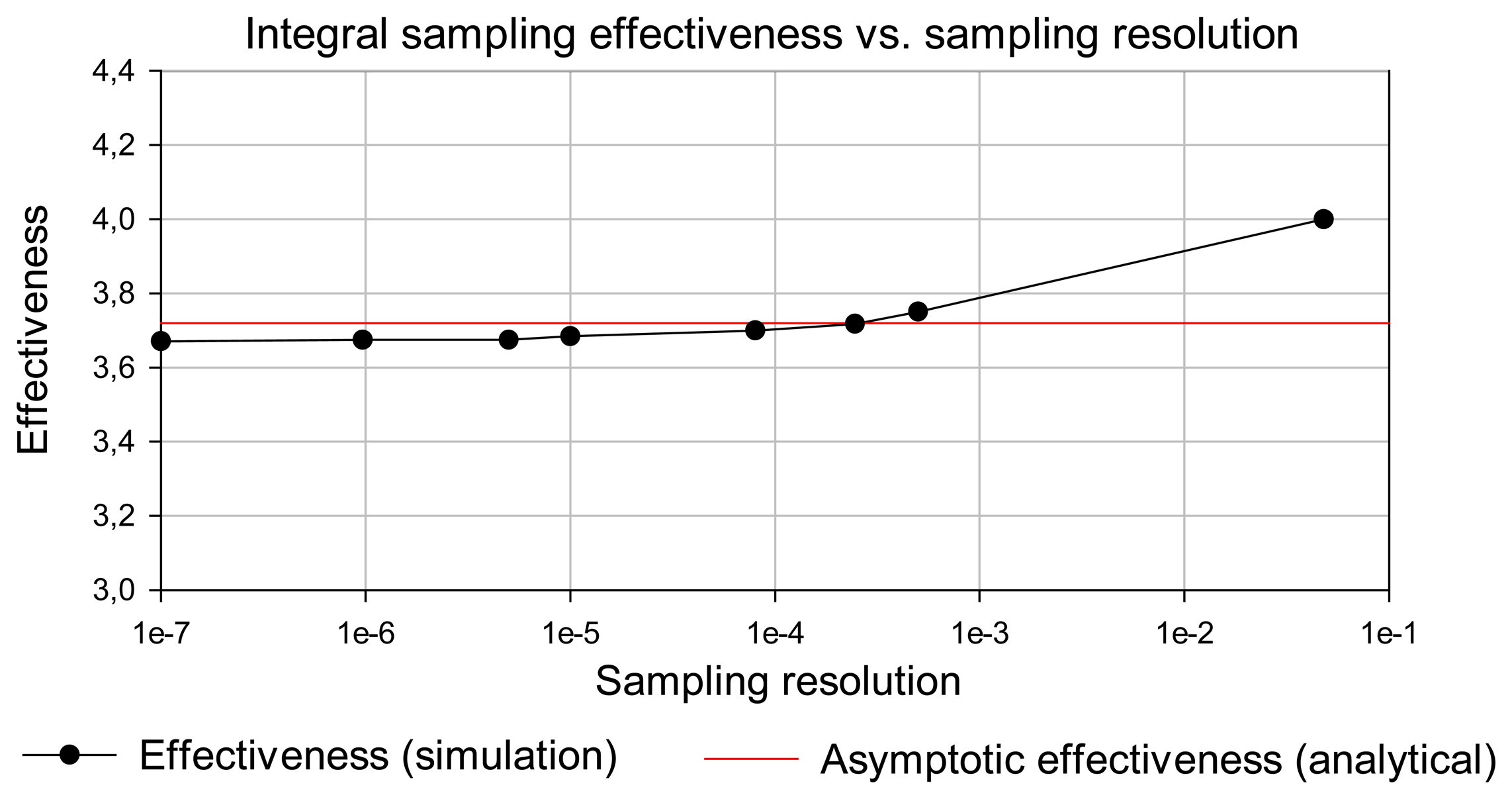
Simulation results of the sampling effectiveness are listed in Table 2 and presented in Fig. 7. The analysis of Fig. 7 shows that the graph of sampling effectiveness approaches the horizontal asymptote for a high sampling resolution. The sampling effectiveness estimated by the simulation for high sampling resolution (for 1/μ = 107) equals 3.671.
For comparison, the asymptotic sampling effectiveness for the tested signal according to (20):
Thus, the simulation result for a high but finite sampling resolution is very close to and consistent with the asymptotic analytical result (29). The analytical approximation of sampling effectiveness calculated above is presented in Fig. 7 as the horizontal line. For comparison, the effectiveness of the linear send-on-delta for the test signal equals 7.02 [3].
6. Application of the analytical formula
On the basis of the formula (20), we have derived analytic solutions of the event-based integral sampling asymptotic effectiveness for particular time responses of the first and second-order dynamic systems modelling environment temporal evolution in many sensory applications.
The following signals are considered:
- -
- step responses of the first-order system, of the differentiation, and of the integration circuits,
- -
- critically damped step responses of the second-order and the nth-order systems,
- -
- second-order overdamped step response,
- -
- undamped step response (harmonic signal).
The results are shown in Table 3. The corresponding results of the send-on-delta effectiveness are reported in [3]. As follows from Table 3, the integral sampling asymptotic effectiveness calculated for the time interval [0,b] is a function of η (or η1 and η2 for the system with different time constants), which is the length of the considered time interval (b) normalized to the appropriate time constants (η, = b/T, η1 = b/T1, η2 = b/T2). Note that the effectiveness for the pure harmonic signal amounts to 1.31 (for a comparison, the effectiveness of the linear send-on-delta for the harmonic wave equals 1.57).
| where: | - the Gamma function, | |
| - the incomplete Gamma function, | ||
| - the error function, | ||
| - the incomplete elliptic integral of the second kind. |
Table 4 shows the integral sampling effectiveness calculated for selected time intervals [0,b]. The time interval selection (except for the undamped system step response) is based on the assumption that b represents the settling time of a system, i.e. the time required for the step response to stay within a specified percentage of its final value. The percentage is shown in the first column, e.g. for the second-order critically damped system, b = 5T is set, because x(5T) = 0.959x0. For the second-order overdamped system, T1/T2 = 7/5 is assumed since x(5T1 = 7T2) = 0.97x0.
The presented results show that the integral sampling effectiveness ranges between 1.31 and 1.93 for signals selected in Table 4 except the effectiveness for the pure linear signal which equals 1. Comparison of the asymptotic integral sampling effectiveness and the minimum send-on-delta effectiveness listed in [3] shows that the former is not greater than the latter for a particular sampled signal as expressed by Theorem 3.
7. Heartbeat sampling
The inherent feature of the event-driven sampling is that the sampling interval can theoretically go to infinity if changes of the monitored signal are fewer than the specified threshold. This feature is opposite to the reliability requirements because it makes it difficult to detect a possible sensor failure. Therefore the event-driven observation strategy is usually equipped with the timeout mechanism.
Namely, if during a specified time interval δtmax the signal x(t) does not change enough in order to trigger the next sample using the integral criterion, the observation is provided according to the time-triggered scheme, which is called heartbeat sampling. In terms of the node reliability, the heartbeat update determines the maximum latency of error detection [13]. Recommendations for heartbeat update in LonWorks networked control systems are specified in [10].
The heartbeat observation especially occurs during the time when the setpoint is reached and the control system stays in the equilibrium state. Thus, if the signal x(t) does not change enough for a long time, the sampling rate is constant and amounts to:
The selection of the heartbeat observation period δtmax is a trade-off between the dependability requirements, stability of the closed-loop system and the available bandwidth or the application performance.
Summing up, the current sampling rate in the event-driven integral sampling for a given signal is included within the range:
Conclusions
The paper presents an analytical method for the estimation of the communication bandwidth and the sampling effectiveness for the event-based integral sampling.
The derived closed-form formulas enable one to allocate the communication bandwidth for a given resolution. The knowledge about the expected bandwidth demands and possible savings allows one to predict a priori its potential usefulness for particular applications. A great challenge for further research is to establish the real-time scheduling and communication for the event-based sampling in order to support the use of irregular observations in time-critical industrial control applications.
References
- Holloway, L.E. The challenge of intelligent sensing of monitoring and control. Proceedings of the 8th IEEE International Symposium on Intelligent Control; 1993; pp. 139–43. [Google Scholar]
- LonWorks Technology Device Data; Rev. 4; Motorola, 1997.
- Miśkowicz, M. Send-on-delta concept: an event-based data reporting strategy. Sensors 2006, 6, 49–63. [Google Scholar]
- Ellis, P.H. Extension of phase plane analysis to quantized systems. IRE Transactions on Automatic Control 1959, 4, 43–59. [Google Scholar]
- Bernhardsson, B. Event triggered sampling. Research problem formulations in the DICOSMOS project; Törngren, M., Sanfridson, M., Eds.; Lund Institute of Technology, 1998. http://www.md.kth.se/∼mis/dicosmos/publications/ET-sampling.pdf.
- Aström, K.J.; Bernhardsson, B. Comparison of periodic and event based sampling for first-order stochastic systems. Proceedings of IFAC World Congress 1999, 301–306. [Google Scholar]
- Akopyan, F.; Manohar, R.; Apsel, A.B. A level-crossing flash asynchronous analog-to-digital converter. Proceedings of IEEE International Symposium on Asynchronous Circuits and Systems; 2006; pp. 12–22. [Google Scholar]
- Allier, E.; Sicard, G.; Fesquet, L.; Renaudin, M. A new class of asynchronous A/D converters based on time quantization. Proceedings of International Symposium on Asynchronous Circuits and Systems; 2003; pp. 196–205. [Google Scholar]
- Otanez, P.; Moyne, J.; Tilbury, D. Using deadbands to reduce communication in networked control systems. Proceedings of American Control Conference; 2002; 4, pp. 3015–3020. [Google Scholar]
- Layer 7 LonMark Interoperability Guidelines; Ver. 3.2. LonMark Interoperability Association, 2002. http://www.lonmark.com/press/download/LYR732.pdf.
- Arzén, K.E. A simple event-based PID controller. Proceedings of IFAC World Congress 1999, 18, 423–428. [Google Scholar]
- Henningsson, T.; Cervin, A. Event-based control over networks: some research questions and preliminary results. Proceedings of Swedish Control Conference Reglermötet'2006, Stockholm; 2006. [Google Scholar]
- Kopetz, H. Real-time systems. Design principles for distributed embedded applications; Kluwer Academic Publications, 1997. [Google Scholar]
- Miśkowicz, M. Adaptive event-triggered algorithms in distributed control network architectures (in Polish). PhD Thesis, AGH University of Science and Technology, Cracow, 2004. [Google Scholar]
- Miśkowicz, M. The event-triggered integral criterion for sensor sampling. Proceedings of IEEE International Symposium on Industrial Electronics; 2005; pp. 1061–1066. [Google Scholar]
- Dorf, R.C.; Farren, M.C.; Phillips, C.A. Adaptive sampling for sampled-data control systems. IEEE Transactions on Automatic Control 1962, 7(1), 38–47. [Google Scholar]
- De Paoli, F.; Tisato, F. On the complementary nature of event-driven and time-driven models. Control Engineering Practice 1996, 4(6), 1996. 847–854. [Google Scholar]
- Savigni, A.; Tisato, F. Kaleidoscope: A reference architecture for monitoring and control systems. Proceedings of the First Working IFIP Conference on Software Architecture; 1999; pp. 369–388. [Google Scholar]
- Mitchell, J.R.; McDaniel, W.L. Adaptive sampling technique. IEEE Transactions on Automatic Control 1969, 14(2), 200–201. [Google Scholar]
- Gupta, S.C. Increasing the sampling efficiency for a control system. IEEE Transactions on Automatic Control 1963, 8(3), 263–264. [Google Scholar]
- Hsia, T.C. Comparisons of adaptive sampling control laws. IEEE Transactions on Automatic Control 1972, 17(6), 830–831. [Google Scholar]
- Hsia, T.C. Analytic design of adaptive sampling control laws. IEEE Transactions on Automatic Control 1974, 19(1), 39–42. [Google Scholar]
- De la Sen, M.; Almansa, A. Adaptive stable control of manipulators with improved adaptation transients by using on-line supervision of the free-parameters of the adaptation algorithm and sampling rate. Informatica, Journal of the Lithuanian Academy of Sciences 2002, 13(3), 345–368. [Google Scholar]
- De la Sen, M. Non-periodic and adaptive sampling. A tutorial review. Informatica, Journal of the Lithuanian Academy of Sciences 1996, 7(2), 175–228. [Google Scholar]
- Dormido, S.; de la Sen, M.; Mellado, Mellado M. Criterios generales de determinación de leyes de maestro adaptivo (in Spanish). Revista de Informática y Automática 1978, 38, 13–29. [Google Scholar]
- Tzafestas, S.; Frangakis, G. Implementing PFM controllers. Control Engineering 1979, 91–104. [Google Scholar]
- Mateo, J.; Laguna, P. Improved heart rate variability signal analysis from the beat occurrence times according to the IPFM model. IEEE Transactions Biomedical Engineering 2000, 47(8), 997–1009. [Google Scholar]
- Jordan, C. Sur la série de Fourier; Comptes Rendus de l'Académie des Sciences. Série Mathématique; 1881; Volume 92, 5, pp. 228–230. [Google Scholar]
- Riesz, F.; Nagy, B. Functional analysis.; New York, Dover, 1990. [Google Scholar]
- Rudin, W. Real and complex analysis.McGraw-Hill Book, 3rd ed.; 1987. [Google Scholar]
- Lunze, J. Robust Multivariable Feedback Control.; Prentice-Hall, 1989. [Google Scholar]
- Boyd, S.; Barratt, C. Linear Controller Design: Limits of Performance.; Prentice-Hall, 1991. [Google Scholar]
- Skogestad, S.; Postlethwaite, I. Multivariable Feedback Control: Analysis and DesignWiley, 2nd ed.; 2005. [Google Scholar]
Figure 1.
Principle of the event-based sampling according to the uniform integral criterion.

Figure 2.
The steady-state sampling error in the level-crossing scheme (a), the example of the event-based sampling according to the integral criterion (b). The sampled signal is the same in both plots (a) and (b), only the time scales are different.
Figure 2.
The steady-state sampling error in the level-crossing scheme (a), the example of the event-based sampling according to the integral criterion (b). The sampled signal is the same in both plots (a) and (b), only the time scales are different.

Figure 3.
The principle of the integral send-on-delta algorithm based on the “upward” event-driven architecture. The messages are broadcasted when the IAE reaches a prespecified threshold.
Figure 3.
The principle of the integral send-on-delta algorithm based on the “upward” event-driven architecture. The messages are broadcasted when the IAE reaches a prespecified threshold.

Figure 4.
Model of the adaptive sampling system.

Figure 5.
Comparison of the adaptive integral sampling (a), and the event-based integral one (b). The “local extremum trap” is illustrated in the adaptive sampling scheme (a). Note that the event-based scheme is immune to the such instability of the sampling error (b). Both sampling schemes are based on the constant integral-difference criterion with the same resolution. The sampled signal is the unit response of the second-order closed-loop system, the maximum sampling period in the adaptive sampling equals Tmax = 0.2[s] ; the zero-order hold is used.
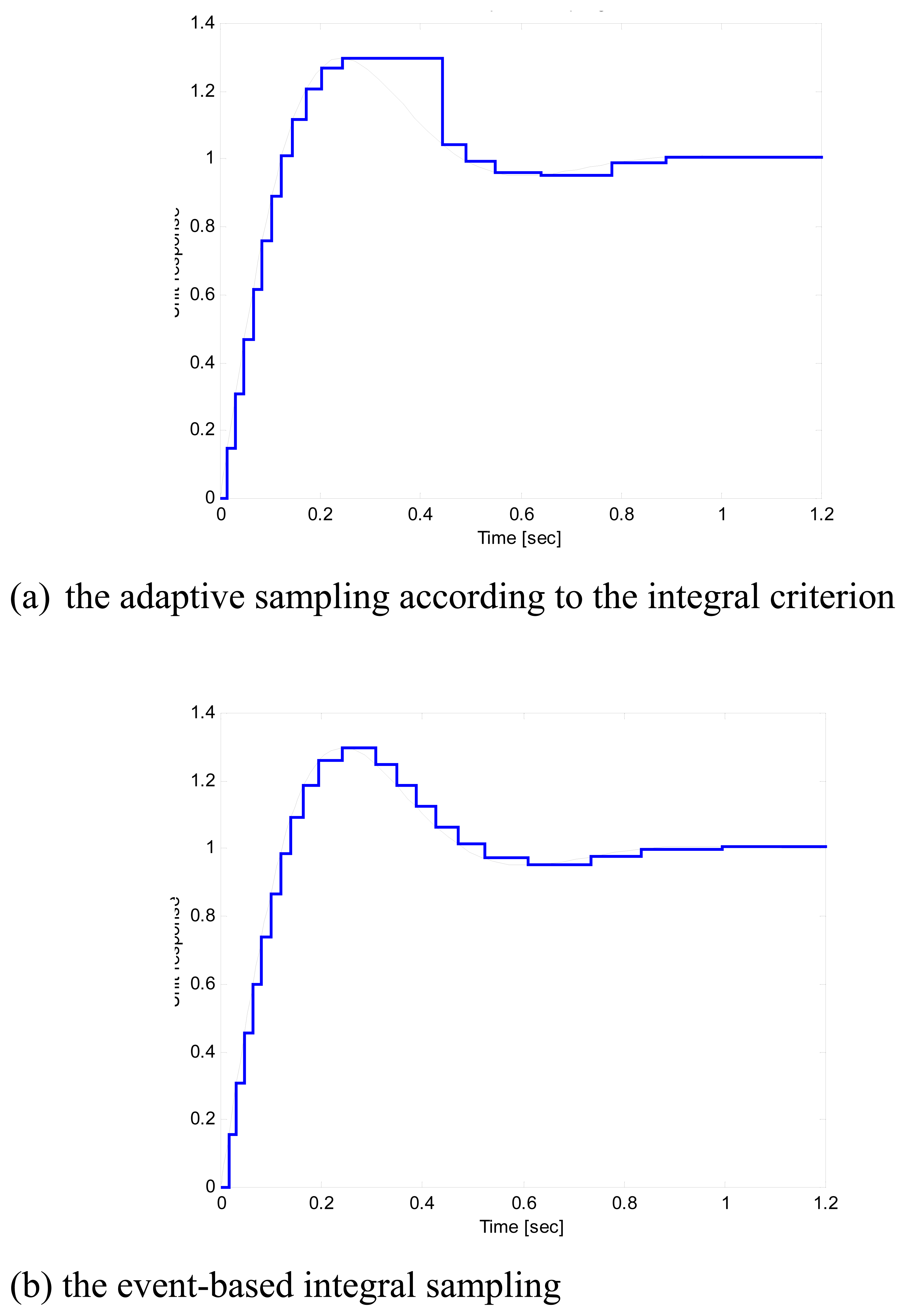
Figure 6.
Simulation results versus analytical approximation of the mean sampling rate according to the integral criterion.
Figure 6.
Simulation results versus analytical approximation of the mean sampling rate according to the integral criterion.
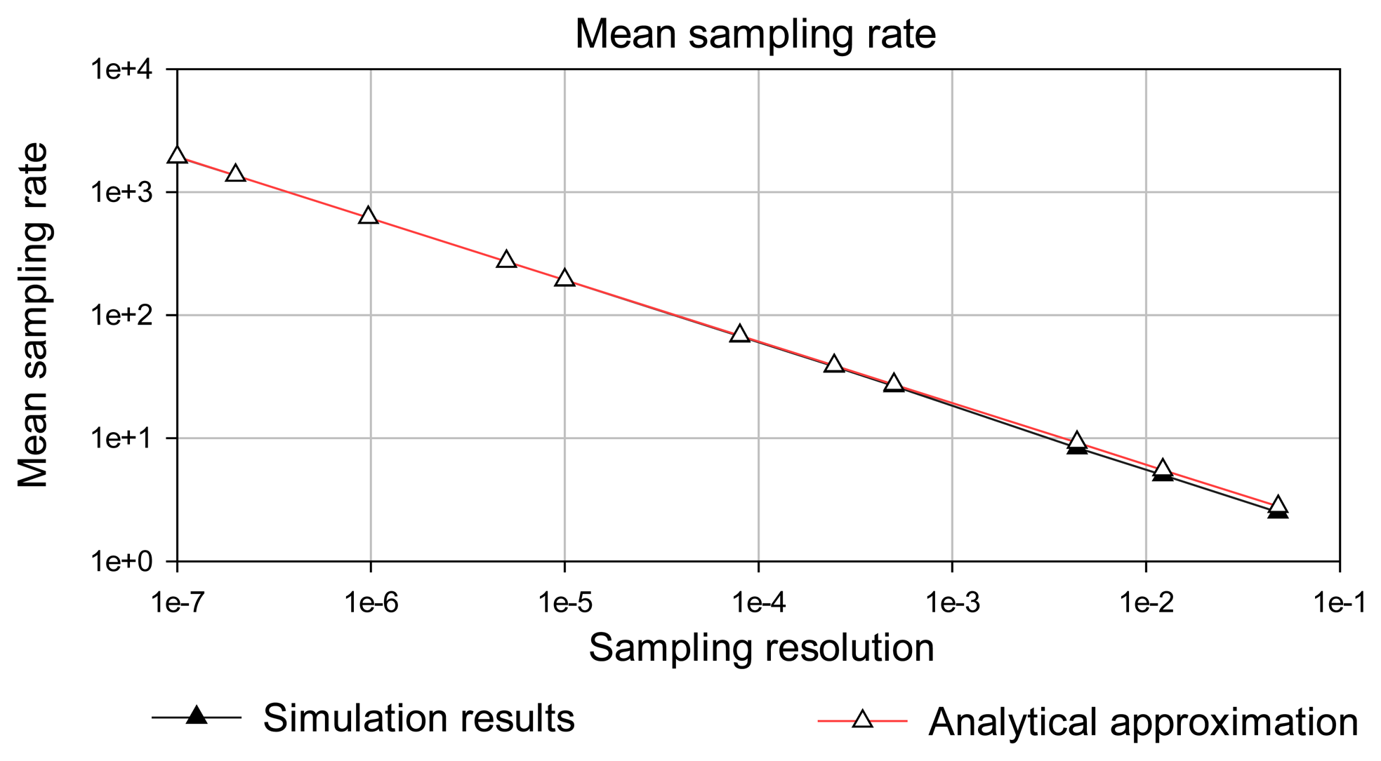
Figure 7.
Simulation results versus analytical approximation for the integral sampling asymptotic effectiveness. The approximation is accurate for small integral absolute error (IAE).
Figure 7.
Simulation results versus analytical approximation for the integral sampling asymptotic effectiveness. The approximation is accurate for small integral absolute error (IAE).

| Integral absolute error (IAE) | Simulation results | Analytical approximation |
|---|---|---|
| 0,048 | 2.5 | 2.78 |
| 1,22E-02 | 5 | 5.52 |
| 4,40E-03 | 8.33 | 9.2 |
| 5,00E-04 | 26.5 | 27.28 |
| 8,00E-05 | 67.5 | 68.2 |
| 5,00E-06 | 272.5 | 272.8 |
| 1,00E-07 | 1925 | 1929 |
| Integral absolute error (IAE) | Number of samples in event-based sampling | Number of samples in periodic sampling | Event-based sampling effectiveness |
|---|---|---|---|
| 0.048 | 3 | 12 | 4.000 |
| 5E-4 | 32 | 120 | 3.750 |
| 2.46E-4 | 46 | 171 | 3.717 |
| 8E-5 | 81 | 300 | 3.700 |
| 1E-5 | 231 | 851 | 3.684 |
| 5E-6 | 327 | 1200 | 3.675 |
| 9.7E-7 | 742 | 2727 | 3.675 |
| 1E-7 | 2310 | 8480 | 3.671 |
Table 3.
The event-based integral sampling asymptotic effectiveness for some time responses of the first and the second-order dynamic systems calculated for the time interval [0,b], where η = b/T, η1 = b/T1, η2 = b/T2.
| Signal | Step response | Asymptotic effectiveness |
|---|---|---|
| First-order step response | ||
| Differentiation circuit | ||
| Integration circuit | ||
| Second-order critically damped step response | ||
| Second-order overdamped step response | ||
| nth-order critically damped step response | ||
| Second-order underdamped step response (0<ξ<1) | Symbolic solution is not available, the numeric solutions for a particular set of parameters can be calculated | |
| x(t) = k(1 − cos ωnt) | Harmonic signal - second-order undamped step response (ξ = 0) |
Table 4.
The event-based integral sampling asymptotic effectiveness for selected time intervals [0,b].
| Signal | Integral sampling effectiveness for selected time intervals |
|---|---|
x(3T) = 0.95x0 | q∞ (η= 3) = 1.93 where: η = b/T |
x(3T) = 0,05x0/T | q∞(η = 3) = 1.93 where: η = b/T |
x (20T) = 0,95·x0t | q∞ (η = 20) = 1.032 where: η = b/T |
x(5T)=0.959x0 | q∞(η = 20) = 1.46 where: η = b/T |
for T1/T2=7/5 : x(5T1=7T2) = 0.97x0 | q∞(η1 = 5, η2=7) = 1.32 where: η1 = b/T1, η2=b/T2 |
x(n = 2, η = 5) = 0.96x0 | q∞ (n = 2, η =5) = 1.46 where η = b/T |
| x(t) = x0 (1−cos ωnt) | q∞ (bωn = πm/2, m = 1,2,…) = 1.31 |
| x(t) = kt | q∞ = 1 |
© 2007 by MDPI ( http://www.mdpi.org). Reproduction is permitted for noncommercial purposes.
Share and Cite
MDPI and ACS Style
Miskowicz, M. Asymptotic Effectiveness of the Event-Based Sampling According to the Integral Criterion. Sensors 2007, 7, 16-37. https://doi.org/10.3390/s7010016
AMA Style
Miskowicz M. Asymptotic Effectiveness of the Event-Based Sampling According to the Integral Criterion. Sensors. 2007; 7(1):16-37. https://doi.org/10.3390/s7010016
Chicago/Turabian StyleMiskowicz, Marek. 2007. "Asymptotic Effectiveness of the Event-Based Sampling According to the Integral Criterion" Sensors 7, no. 1: 16-37. https://doi.org/10.3390/s7010016