An EMI Filter Selection Method Based on Spectrum of Digital Periodic Signal

1
Ministry of Defence, Administration for Civil Protection and Disaster Relief, Vojkova cesta 61, 1000 Ljubljana, Slovenia
2
University of Maribor, Faculty of Electrical Engineering and Computer Science, Smetanova ulica 17, 2000 Maribor, Slovenia
3
ISKRAEMECO d.d, Research and Development Department, Savska loka 4, 4000 Kranj, Slovenia
*
Author to whom correspondence should be addressed.
Sensors 2006, 6(3), 90-99; https://doi.org/10.3390/s6030090
Submission received: 20 January 2006
/
Accepted: 2 March 2006
/
Published: 3 March 2006
Abstract
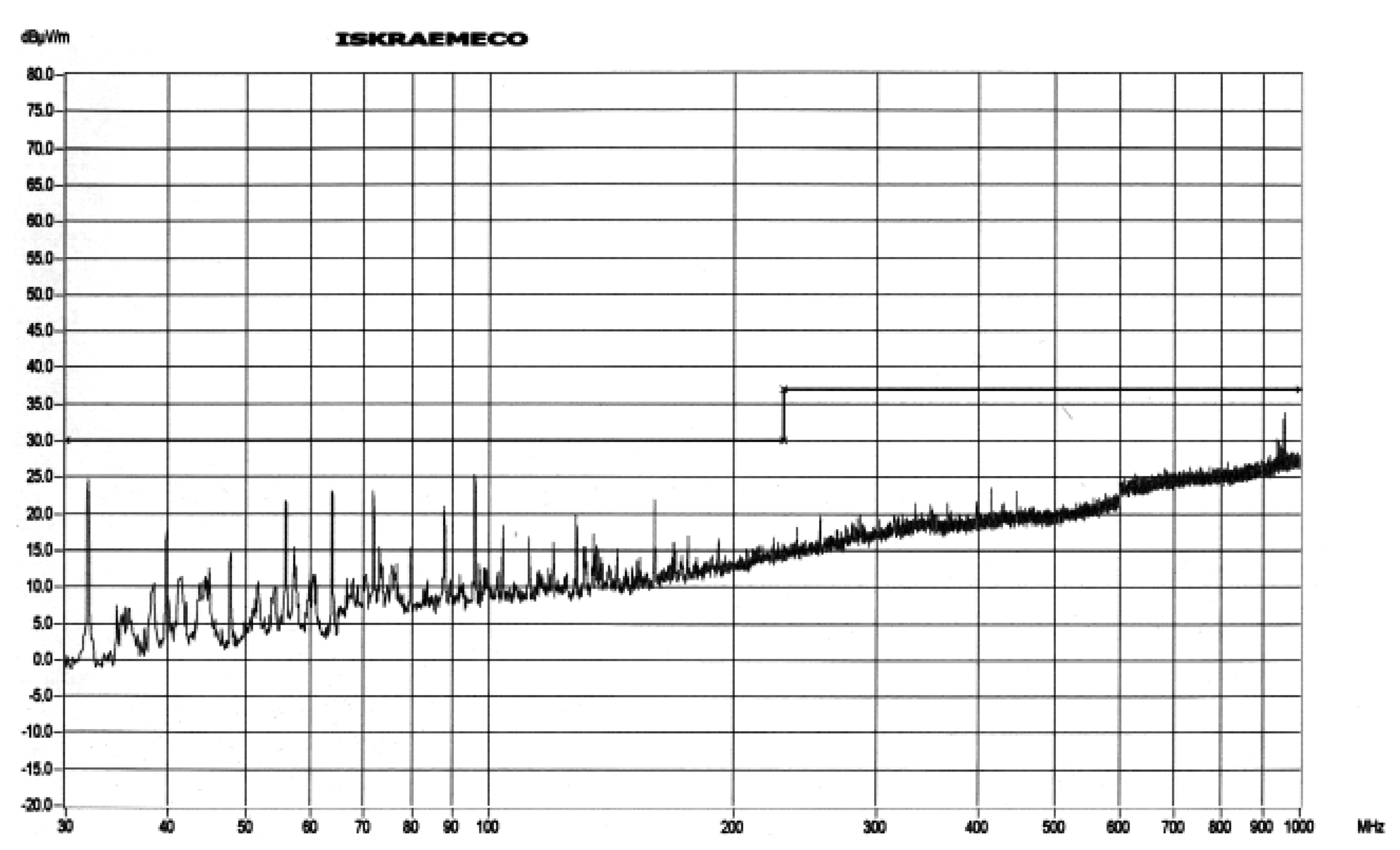
:This paper describes a new method for the selection of an appropriate signal line Electromagnetic Interference (EMI) filter. To date, EMI filter selection has been based on the measurement of the radiation of the entire device. The new selection method based on the signal's Fast Fourier Transform (FFT) measurement has proved to be efficient. The EMI filter is optimized separately for each line. The method described in this paper involving a Central Processor Unit (CPU) module demonstrates that the proposed FFT-based selection method is better than the radiation-based one. The radiation level in the frequency range 30 MHz to 1 GHz is lower for approximate 2 – 6 dBμV/m.
1. Introduction
When we develop small devices such as sensors we are often confronted with Electromagnetic Compatibility (EMC) problems because components are placed very close to each other. To some extent these EMC problems can be solved with suitable component selection method and printing circuit board design. When this does not solve the problems EMI filters must be used. They must be placed near noise sources such as microcomputers, digital drivers, oscillators, input-output lines, etc.
There are three EMI filter selection methods. The first method uses ground plane for EMI filter construction. It is described in Chapter 2 of this paper. The second one is based on radiation measurements. The radiation of the entire device is measured, which provides a discrete frequency component with the maximum amplitude. The EMI filter with maximum insertion loss close to this discrete frequency component is selected. The resulting filters have the same frequency characteristics within the entire device. The third method has been developed and tested in the EMC Laboratory of the ISKRAEMECO d.d. Company. It is based on the FFT measurements on a single signal line.
The main advantage of the new method is that a filter is selected for each single line separately. This gives better results in terms of EMC problem solving than the other two methods. It is very important that this new EMI filter selection method and all other recommendations for good EMC design are used in the early development phase of a product such as sensor.
2. The Grounding
Correct grounding is critical to EMC problem solving. Every signal line must be surrounded by ground (Figure 1). In this way the sufficient capacitive shunting of the high-frequency noise to ground is achieved [1-3]. The capacitive shunting is more effective when the joint path of the signal line and ground is longer. Such capacitive shunting serves as some sort of EMI filter, but is often insufficient. In such cases, real EMI filters should be used.
3. Critical Line Length
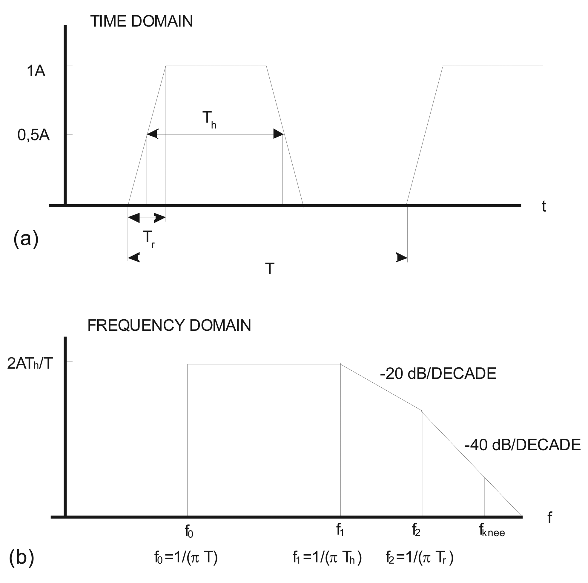
The expression “critical line length” is known from high-speed transmission line theory [4-6]. The qualification of a transmission line as a long transmission line depends on transported frequencies. Figure 2a shows a digital periodic signal (a trapezoidally-shaped wave) and figure 2b shows its frequency spectrum [7].
The spectrum consists of discrete frequency components fn = nfT, where fT = 1/T. By drawing asymptotes of the spectrum, we get a horizontal line up to the first corner frequency (Figure 2b)
and from there a descending line at the rate of decrease of 20 dB/dec. up to the second corner frequency (Figure 2b)
For higher frequencies, the rate of decrease is 40 dB/dec. (Figure 2b).
Frequency fknee is a practical maximum which is about 1.5 times f2.
The critical line length is determined by the frequency fknee. It is well known that electromagnetic emission increases with frequency until half the wavelength of the signal exactly fits the length of the trace.
The propagation of the line is
Tpd is the propagation delay. The wavelength in Equation (5) can be written as
At the critical line length the rise time Tr exactly matches the two-way propagation delay time Tpd (source – load – source). This means that the transient phenomenon formed by the low-to-high signal transition precisely fits the line length. For that reason, this distance (the critical line length) is referred to as the length of the rising edge [4-6].
To simplify Equation (8), the real value of propagation delay for FR-4 – currently the most commonly used material in the production of printed circuit boards (PCBs) – is used. With equations (9) and (10) the maximum electrical line length before the required line termination is determined. The calculations below are used for the dielectric constant of FR-4 material (εr=4.6). The latter varies with signal frequency within the material. Most engineers generally assume εr to be in the range of 4.5 to 4.7. These are the values that are published in various technical references [8].
A line length equal to or longer than the critical length definitively behaves as a transmission line. Characteristic impedance, delay and reflections should not be ignored. At the same time, it also behaves as an efficient antenna and is reflected in considerable electromagnetic radiation and susceptibility problem. Corrupted signals are usually rich on higher frequency components.
4. Typical Frequency – Observed as EMI
Typical frequency – observed as EMI – is a frequency at which most EMI-related problems can be expected [8]. It depends on the logic elements and microcontroller used. More precisely, it is dependent upon the rise time of the signals transmitted by these elements (11). Special attention should therefore be paid to the selection of appropriate logic elements and microcontroller. If, for instance, a faster High-speed CMOS with TTL inputs (HCT) instead of a slower Low-power Schottky transistor-transistor logic (LS-TTL) is used, the electromagnetic emission can increase up to three times. As might be expected, a discrete frequency component at typical frequency starts to emit electromagnetic disturbances at a certain line length at which it becomes an efficient antenna [8].
These typical frequencies – observed as EMI – are very important when designing an electronic circuit.
To check the accuracy of the Equation (11), the amplitude of the discrete frequency component at the typical frequency – observed as EMI – was measured [9]. The measurement equipment proved to be inadequate. We measured with four channels oscilloscope Tektronix TDS744A with maximum digitizing rate 2 GS/s and analog bandwidth 500 MHz. This was too low for 74 Advanced CMOS (74AC) logic with a typical frequency of 1.6 GHz. For that reason the 74HC logic with a typical frequency of 270 MHz was chosen.
Figure 3 shows the output signal from 74HC245 logic circuit. The frequency spectrum rises again at frequencies in the range 220–300 MHz. The peak with the amplitude of 28.64 dB is located at the typical frequency of 265.258 MHz.
The measured signal rise time tr was 12 ns. The result of the calculation of the typical frequency – observed as EMI (11) – is 265.258 MHz (12). The calculated value is the same as the measured one.
The calculation of the typical frequency – observed as EMI – is relatively simple. Its accuracy was also confirmed by the measurement.
5. Adjustments and Filtering
So far no attention has been paid to the filter adjustments [10]. Also, due to rather slow processors (up to 24 MHz) and small printed circuit boards (short antennas) used in the ISKRAEMECO d.d. production, the input impedances have not been calculated yet.
EMI filters have been placed near the noise source on all signal lines exceeding the critical line length (lmax). The adjustments can also be further improved by a proper EMI filter selection. In addition, attention has to be paid to the EMI filter structure.
EMI filter insertion losses are handled at 50Ω input and output impedance [11-12]. Normally, such impedance does not exist in real electronic circuits. It is a well-known fact that EMI filter performance strongly depends on the input and output impedance. This is the impedance of the surrounding electronic circuit. Some general rules for selection of an appropriate EMI filter structure should be considered (Figure 4) [13-14]. The fact is that capacitors are best used in high impedance circuits, whereas coils are best used in low impedance circuits. The reason lies in component characteristics at high frequencies [8]. A suitable EMI filter structure can be selected using the table in Figure 4.
6. Proper EMI Filter Selection
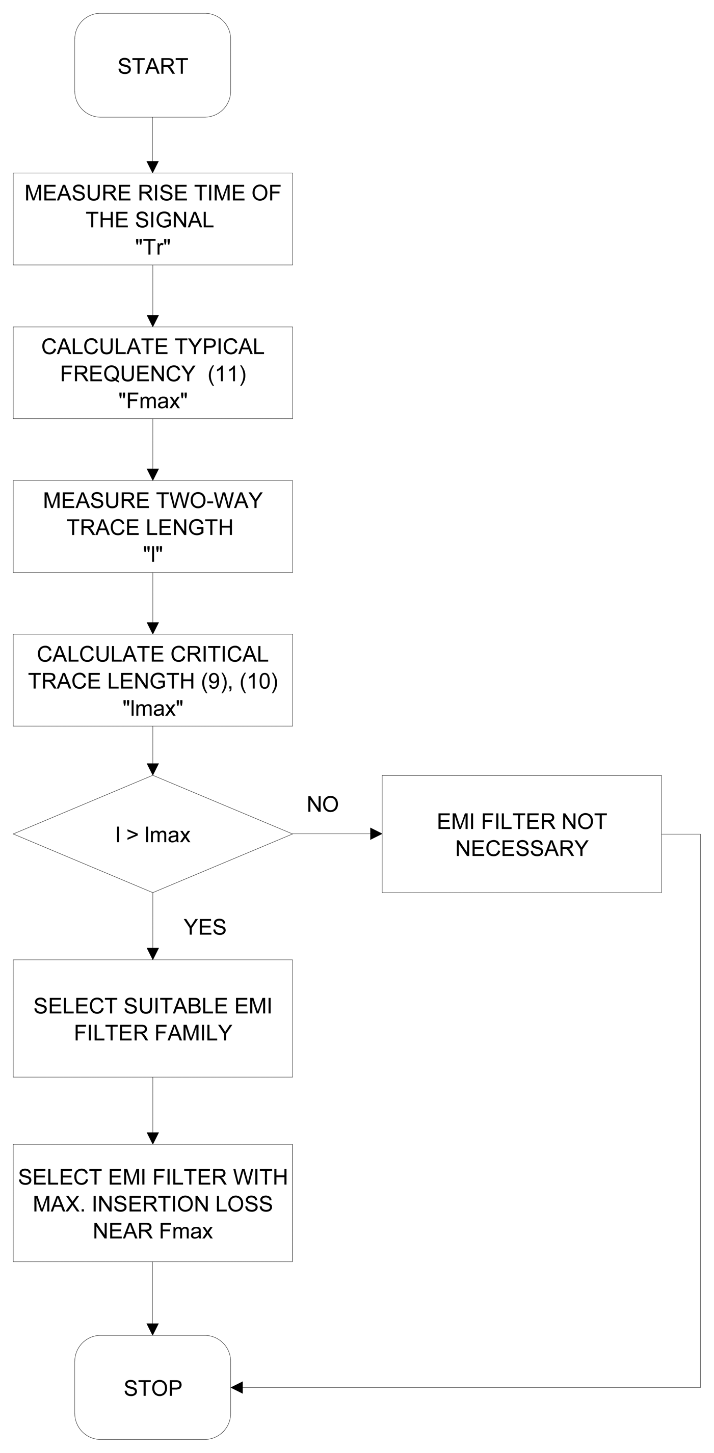
The procedure for a proper EMI filter selection consists of the following steps:
- Measurement of the signal rise time tr;
- Calculation (or measurement) of the typical frequency – observed as EMI;
- Selection of a suitable EMI filter family with regard to the application requirements;
- Selection of an EMI filter from the family which has the maximum insertion loss at the approximate typical frequency.
The need for the use of EMI filters depends upon the critical line length which has been verified in practice [15]. If a two-way line length is shorter than the previously calculated lmax (critical line length) and if there are no via connections on the line, the use of an EMI filter is not necessary.
Figure 3 shows FFT of the 74HC245 logic circuit output signal. EMI filter was added to the signal line. The filter was selected according to the above-described procedure. The Murata EMI filter NFW31SP506X1E4 with the maximum insertion loss at the frequency of about 250 MHz was used. Figure 5 shows that the level of the harmonic component at the typical frequency has reduced from 28.64 dB to 21.20 dB, proving that the use of EMI filter was a good idea.
The described EMI filter selection procedure is shown in Figure 6.
7. Conclusions
Generally, a selection of suitable EMI filters is very important for designing. The tests performed on the CPU module clearly demonstrate that the proposed FFT-based EMI filter selection method is better than the radiation-based one. We used CPU module with 24 MHz, 32 bits microcontroller (Motorola MC 68332) on the eight layer printed circuit board.
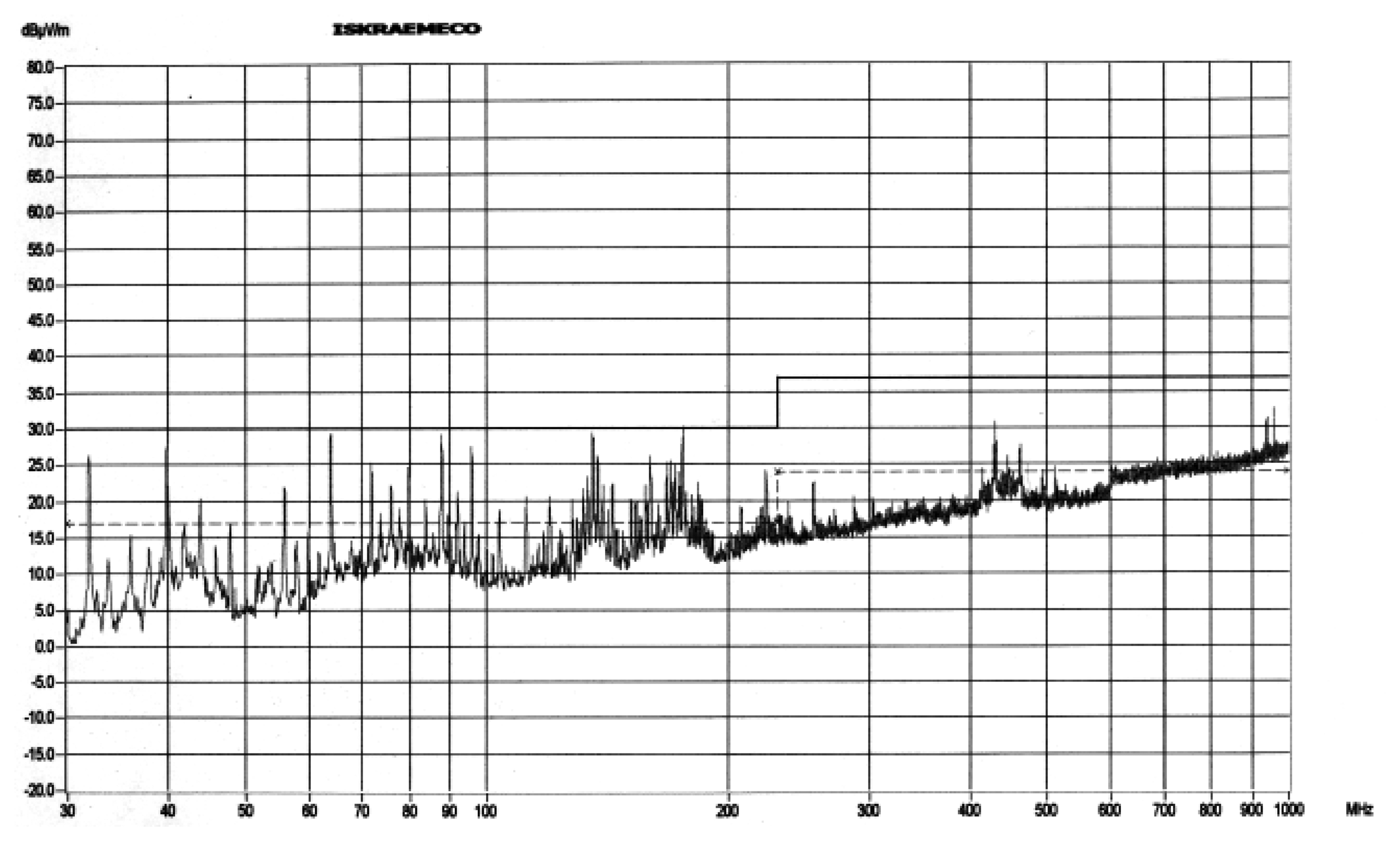
First, CPU module was equipped with EMI filters selected with the radiation-based method and the radiated emission was measured (Figure 7). It was below the allowed limit but still rather high. Next, EMI filters selected according to the new method were installed in the same CPU module. As expected, the radiation level was significantly lower (Figure 8).
The main advantage of this method is that it solves EMC emission problems separately for each single signal line, which is why we believe it produces better results.
Acknowledgments
EMI filter selection method described in this paper was developed in the EMC Laboratory of the ISKRAEMECO d.d. Company and in the Electrical Measurements Laboratory, Faculty of Electrical Engineering and Computer Science, University of Maribor, and I thank them both.
References
- Campbell, D.; Kreidl, H. Solving EMC Issues. Workshop 36, EMV'03, Augsburg; 2003; p. 116. [Google Scholar]
- Morrison, R. Grounding and Shielding Techniques.; John Wiley & Sons: New York, 1998. [Google Scholar]
- Britt, S. D.; Hockanson, D. M.; Sha, F.; Drewniak, J. L.; Hubing, T. H.; Van Doren, T. P. Effects of Gapped Groundplanes and Guard Traces on Radiated EMI. IEEE International Symposium on Electromagnetic Compatibility; 1997. [Google Scholar]
- Buesink, F. J. K. High Speed Digital Design Topics for Printed Circuit Boards. Workshop 24, EMV'01, Augsburg; 2001; pp. 11–12. [Google Scholar]
- Anderson, E. M. Electric Transmission Line Fundamentals.; Reston, 1985. [Google Scholar]
- Chipman, R. A. Theory and Problems of Transmission Lines; Schaum's Outline Series; McGraw-Hill, 1968. [Google Scholar]
- Kaiser, K. L. Electromagnetic Compatibility Handbook.; CRC press: New York, 2004; Chapter 12; pp. 155–165. [Google Scholar]
- Montrose, M. I. EMC the printed circuit board: Design, Theory, and Layout Made Simple.; IEEE Press Editorial Board: New York, 1999; Chapters 1, 3, 6, 7. [Google Scholar]
- Kazama, S.; Shinohara, S.; Sato, R. Evaluation of methods of measuring digital IC terminal output.; EMC Research Laboratories Co., Ltd.: Sendai, Japan, 2000; pp. 329–334. [Google Scholar]
- Anderson, D.; Smith, L.; Gruszynski, J. S-Parameter Techniques for Faster, More Accurate Network Design.; Hewlett-Packard Company: New York, 1996-1997; pp. 4–13. [Google Scholar]
- Desnica, V. D.; Zivanov, L. D.; Aleksic, O. S.; Lukovic, M. D.; Nimrihter, M. D. Comparative Characteristics of Thick-Film Integrated LC Filters. IEEE Transactions on Instrumentation and Measurement 2002, 51(4), 570–576. [Google Scholar]
- Caggiano, M.; DelGiudice, B.; Tornquist, K. Modeling the power and ground effects of BGA packages. IEEE Trans. Adv. Packag. 2000, 23(2), 156–163. [Google Scholar]
- Antonini, G. SPICE Equivalent Circuits of Frequency – Domain Responses. IEEE Transactions on Electromagnetic Compatibility 2003, 45(3), 502–512. [Google Scholar]
- Murata. Noise Suppression by EMI Filtering: Basics of EMI Filters. No. TE04EA-1 1998, 1–4. [Google Scholar]
- Hall, S. H.; Garret, W. H.; James, A. M. High-Speed Digital System Design: A Handbook of Interconnect Theory and Design Practices. ; John Wiley & Sons: New York, 2000. [Google Scholar]
Figure 1.
Correct grounding.
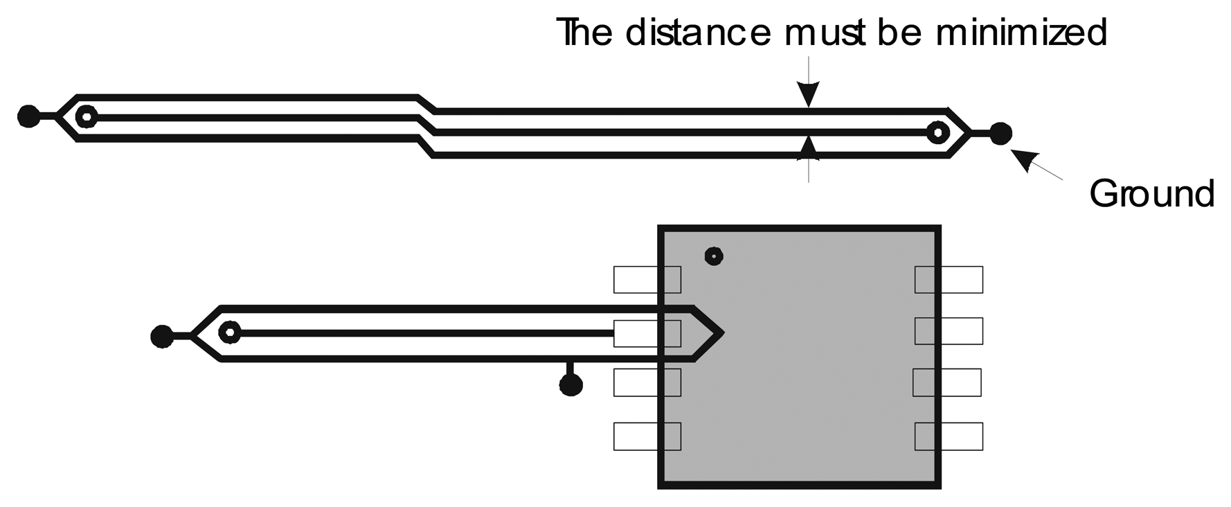
Figure 2.
Spectrum of digital periodic signal.

Figure 3.
FFT of an output signal from 74HC245 logic circuit.

Figure 4.
Selection of an appropriate EMI filter structure.
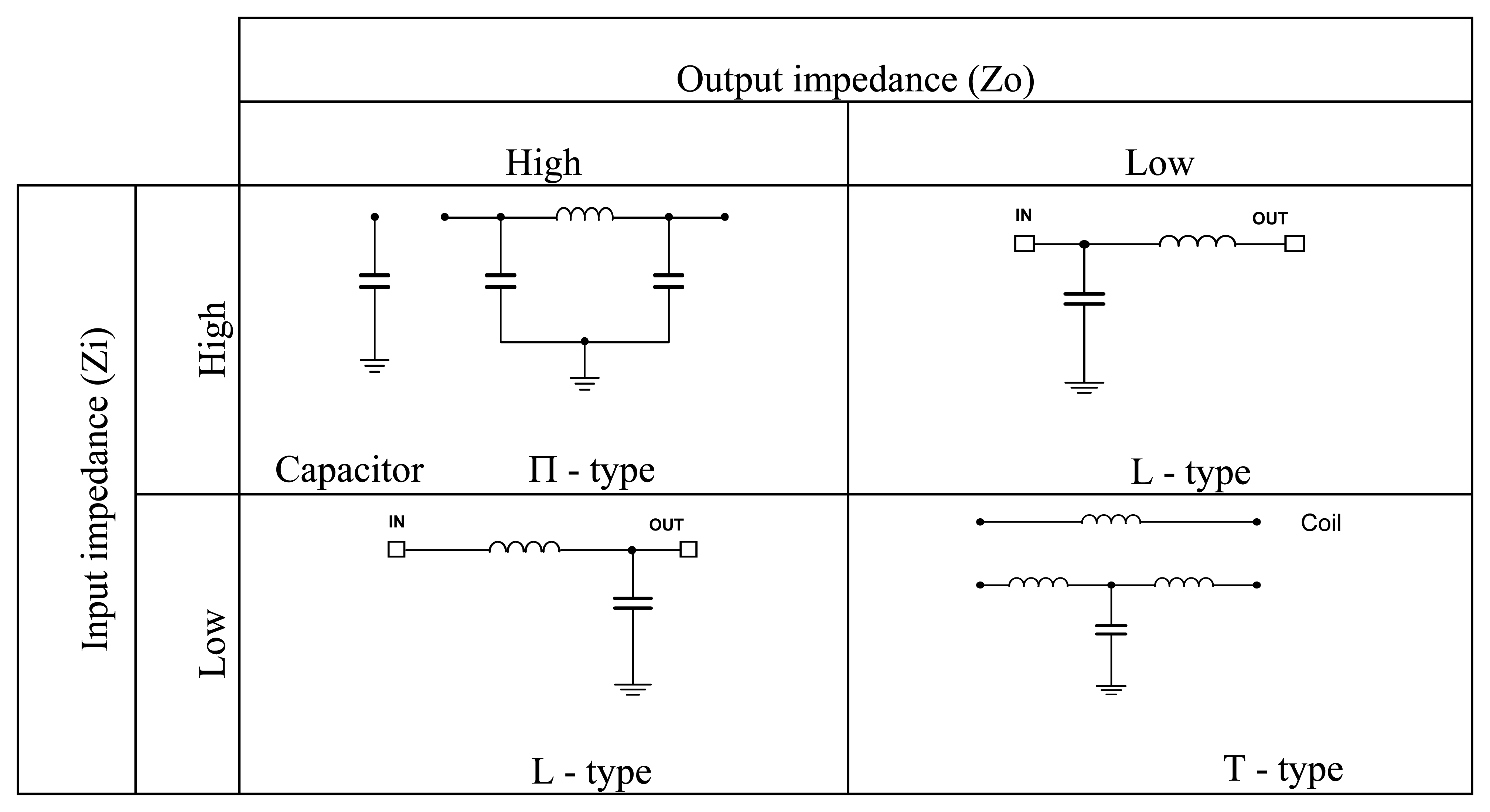
Figure 5.
FFT of a signal that has passed through the Murata EMI filter NFW31SP506X1E4 – an output from 74HC245 logic.
Figure 5.
FFT of a signal that has passed through the Murata EMI filter NFW31SP506X1E4 – an output from 74HC245 logic.
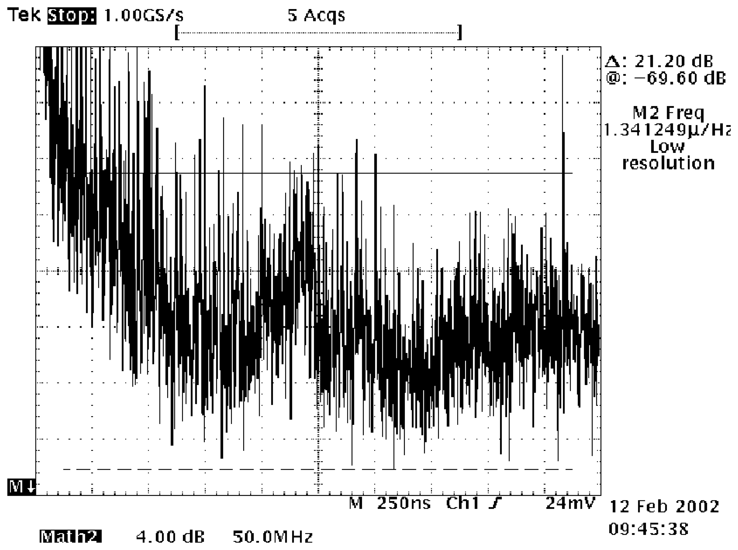
Figure 6.
EMI filter selection flow chart.

Figure 7.
Radiated emission (radiation-based method).

Figure 8.
Radiated emission (new method).

© 2006 by MDPI ( http://www.mdpi.org). Reproduction is permitted for noncommercial purposes.
Share and Cite
MDPI and ACS Style
Podbersic, M.; Matko, V.; Segula, M. An EMI Filter Selection Method Based on Spectrum of Digital Periodic Signal. Sensors 2006, 6, 90-99. https://doi.org/10.3390/s6030090
AMA Style
Podbersic M, Matko V, Segula M. An EMI Filter Selection Method Based on Spectrum of Digital Periodic Signal. Sensors. 2006; 6(3):90-99. https://doi.org/10.3390/s6030090
Chicago/Turabian StylePodbersic, Marko, Vojko Matko, and Matjaz Segula. 2006. "An EMI Filter Selection Method Based on Spectrum of Digital Periodic Signal" Sensors 6, no. 3: 90-99. https://doi.org/10.3390/s6030090