Novel Planar Electromagnetic Sensors: Modeling and Performance Evaluation


Institute of Information Sciences and Technology, Massey University, Palmerston North, New Zealand
Sensors 2005, 5(12), 546-579; https://doi.org/10.3390/s5120546
Submission received: 5 December 2005
/
Accepted: 15 December 2005
/
Published: 15 December 2005
Abstract
:High performance planar electromagnetic sensors, their modeling and a few applications have been reported in this paper. The researches employing planar type electromagnetic sensors have started quite a few years back with the initial emphasis on the inspection of defects on printed circuit board. The use of the planar type sensing system has been extended for the evaluation of near-surface material properties such as conductivity, permittivity, permeability etc and can also be used for the inspection of defects in the near-surface of materials. Recently the sensor has been used for the inspection of quality of saxophone reeds and dairy products. The electromagnetic responses of planar interdigital sensors with pork meats have been investigated.
1. Introduction
Nondestructive testing or NDT is defined as the use of noninvasive techniques to determine the integrity of a material, component or structure or quantitatively measure some characteristics of an object. So in short NDT does inspect or measure without doing any harm or damage of the system. In recent times NDT has been applied in many different branches of industry. With the increasing demand for highly reliable and high performance inspection techniques, during both manufacturing, production and use of a system or structure, the demand for the employment of suitable NDT techniques is increasing. The use of NDT is even more indispensable in the case of structures that have to work in severe operating environments. There are NDT applications at almost any stage in the production or the life cycle of a component. Some of the most important areas are:
- Power stations – nuclear and conventional power plants.
- Petro-chemical industry.
- Transportation – railways.
- Food industry - Quality assurance of food products.
- Medical sciences.
- Civil engineering - inspection of concrete structures, bridges, infrastructure due to aging problem.
- Aircraft - fatigue estimation in aircraft surface and other parts.
- Pipe inspection - Inspection of pipes and piping systems in industrial plants. The pipes are used for carrying oils, gases, waters, milks etc.
- Others.
There are different NDT techniques available with different characteristics. The following are the most commonly used NDT techniques: Visual, Magnetic, Ultrasonic, Acoustic, Radiography, Eddy current and X-ray. The type of technique to be used entirely depends on the specific application.
For last few years the author has been working on the design, fabrication and employment of planar type electromagnetic sensors. The outcomes have been successfully applied in many applications such as the inspection of printed circuit boards [7, 8, 9], estimation of near-surface material properties [10, 11], electroplated materials [12, 13], saxophone reed inspection [14], inspection of dairy products [15]. The planar interdigital sensors have been used for the non-invasive estimation of fat content [16]. This paper will describe a few of those applications.
2. Configuration and Operating Principle of Planar Electromagnetic Sensors
Three planar types of sensors, meander, mesh and interdigital, have been designed and fabricated to study the interaction of these sensors on conducting, magnetic and dielectric materials. The sensors are of planar type and have a very simple structure. They have been fabricated using simple printed circuit board (PCB) fabrication technology. The operating principle of these sensors is based on the interaction of the electromagnetic field generated by the sensors with the neighboring materials under investigation. Meander, mesh, interdigital or a combination of the three can be used depending on the application.
The representation of the mesh and meander type sensors are shown in figure 1. The mesh and meander type sensors consist of two coils: one coil is known as the exciting coil and the other coil is known as the sensing coil. The exciting coil carries alternating current and generates a high frequency electromagnetic field penetrates in to the system under test. The induced electromagnetic field in the testing system will generate eddy currents on the system under test, given that the material under test is of conducting or magnetic type. Due to the flow of eddy current the induced field in the testing system will modify the generated field, and the resultant field will be detected by the pick-up coil or sensing coil, which is placed above the exciting coil.
The sensor can be either of a meander type or of a mesh type, the type of sensors to be chosen depends on the applications. Meander type sensing coils used for testing the integrity of materials has been reported in [1-3, 9, 10]. If the meander type sensor is used to detect cracks in a metal, the disadvantage is that the performance of the sensor is not independent of the alignment of the cracks or non-homogeneity of the material structure (in the process of evaluating material integrity), with respect to the sensor configuration. To overcome this problem the mesh type sensor has been developed [11, 17-20]. In the mesh type sensor the eddy currents take a more circular pattern thus dismissing the geometry/alignment effects encountered in meander type sensors, with the material under test.
The structural configuration of the planar type sensor is shown in figure 2. The exciting coil and the sensing coil are separated by a polyimide film of 50μm thickness. In order to improve the directivity of flux flow a magnetic plate of NiZn is placed on top of the sensing coil. The size of the sensor depends on the number of pitches used in that. The optimum pitch size depends on the application [17, 18].
Four types of sensors of varying lengths and pitches (tables 1 and 2) were designed on Protel DXP 2004.
It is seen from the diagrams that the coils are connected to a Bayonet Neill Concelman (BNC) connector. The AC voltage source drives the exciting coil. The current through the exciting coil is measured across a resistor of an appropriate value connected in series with the exciting coil. The output voltage is measured across the sensing coil. The two coils (exciting and sensing) are designed on top of each other but on opposite sides. On the schematics above the color blue represents the exciting coil while red represents the sensing coil. The exciting coil cannot be seen as the sensing coil overlaps on it. The fabricated sensors are shown in figures 3 and 4 respectively.
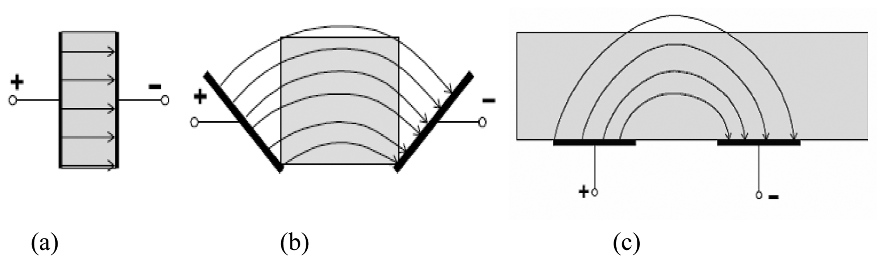
The operating principle behind the interdigital sensor is very similar to the one observed in a parallel plate capacitor [21-26]. Figure 5 shows the relationship between a parallel plate capacitor and an interdigital sensor, and how the transition occurs from the capacitor to a sensor [23]. There is an electric field between the positive and negative electrodes and figure 5a, b and c shows how these fields pass through the material under test (MUT). Thus material dielectric properties as well as the electrode and material geometry affect the capacitance and the conductance between the two electrodes.
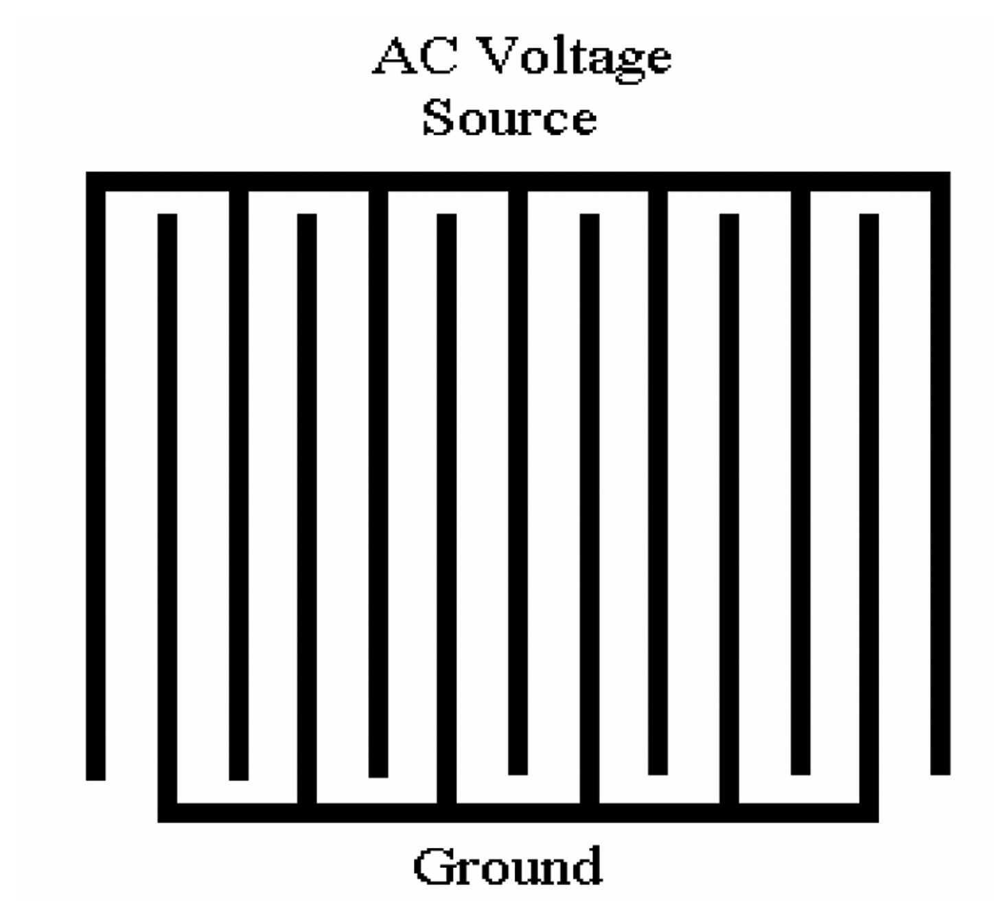
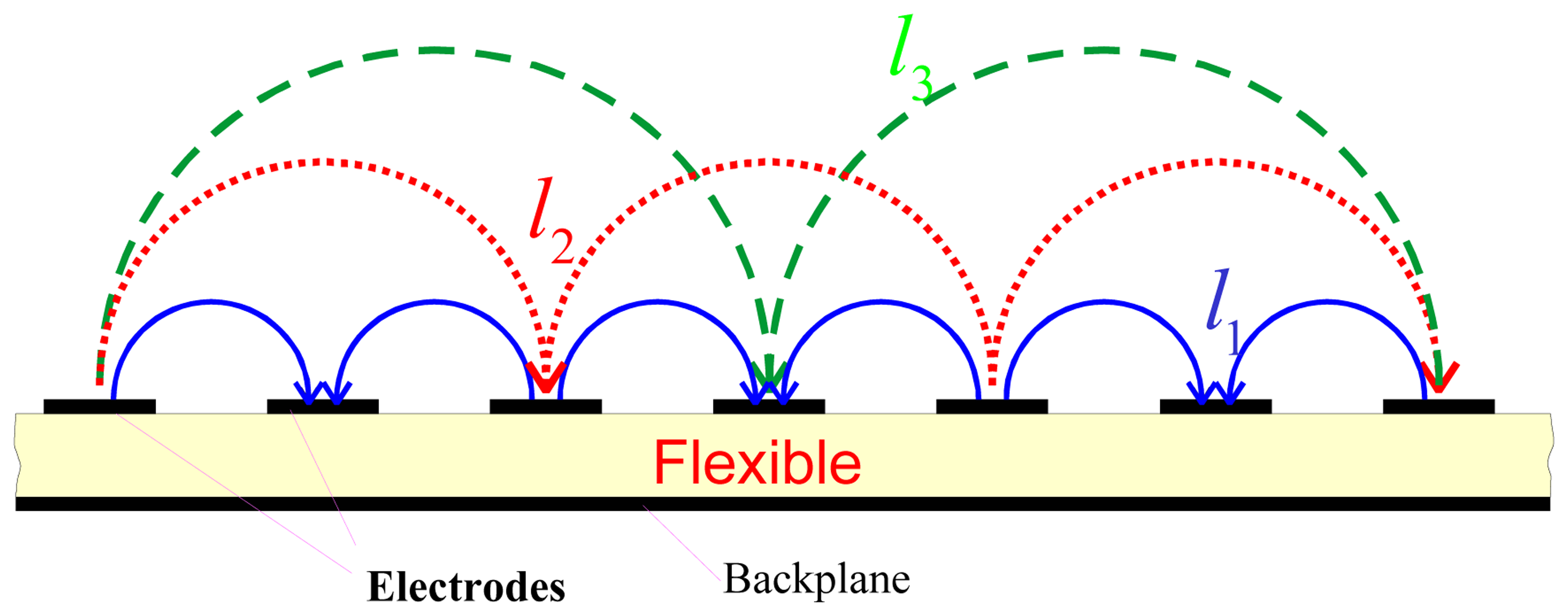
The electrodes of an interdigital sensor are coplanar. Hence, the measured capacitance will have a very low signal-to-noise ratio. In order to get a strong signal the electrode pattern can be repeated many times. This leads to a structure known as an interdigital structure in which one set of electrodes are connected or driven by an AC voltage source while the other set are connected to ground as shown in figure 6. An electric field is formed between the driven and the ground electrodes. This can be seen more clearly in figure 7. It can be seen that the depth of penetration of the electric field lines vary for different wavelengths. The wavelength (λ) of interdigital sensors is the distance between two adjacent electrodes of the same type. In figure 7 there are three lengths (l1, l2 and l3) showing the different penetration depths with respect to the wavelength of the sensor.
Planar interdigitated array electrodes have many applications such as complex permittivity characterization of materials [24], gas detection [25], determining components in aqueous solutions [26], estimation of fiber, moisture and titanium dioxide in paper pulp [27, 28] etc.
Four interdigital sensors of different wavelengths and lengths were designed on Protel DXP 2004. The sensor parameters are shown in table 3 below. The sensor schematic is shown in figure 8.
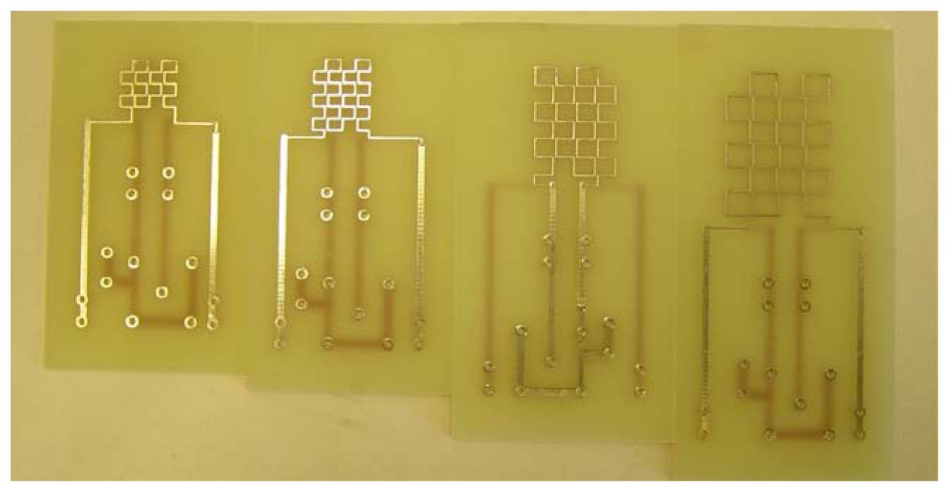
The schematic diagram in figure 8 shows an interdigital sensor with 9 electrodes. Four electrodes act as the excitation/driving electrodes. The other five electrodes are connected to ground. When there is a material between the electrodes the electric fields from the driving electrodes penetrates through most of the material that is under test, and then terminates on the sensing electrodes. The electric field lines are affected by the dielectric properties of the material under test. Thus the potential or the current at the sensing electrodes is also a function of the material's dielectric properties. The advantage of using interdigital sensors is that it has only one sided access to the material under test. Fabricated sensors are shown in figure 9.
3. Analysis of planar sensors using finite element modeling software
In this section the characterization of all types of sensors, meander, mesh and interdigital types have been carried out using finite element modeling. Before experimentation all three sensors are modeled to analyze the distribution of electric field and magnetic flux. The finite element software FEMLAB by COMSOL [27] is used to model and analyze the field distribution of all three types of sensors.
Quasi-static analysis is used for the modeling of the three types of sensors. In quasi-static analysis it is assumed that
Hence Maxwell's equations can be written as:
B, H, Je, D, E, σ, ν and ρ denote magnetic flux density, magnetic field strength, externally applied current density, electric flux density, electric field intensity, electrical conductivity, velocity of the conductor and volume charge density respectively.
Using the definitions of the potentials, we have
And the relationship between magnetic field, magnetic field strength and magnetization (M), we get
Ampere's law can be rewritten as
Where A = magnetic vector potential and μ0 is the magnetic permeability of free space.
Taking the divergence of the equation above gives the equation of continuity
Introducing two new potentials
When substituted into equations (7) and (8) they give the same electric and magnetic fields,
A particular gauge is chosen to obtain a unique solution. This means that constraints are put on Ψ. A constraint can also be put on ∇.A. If both ∇.A and ∇ × A are given a vector field can be uniquely defined up to a constant (Helmholtz's theorem).
The inductance (mesh and meander) and capacitance (interdigital) are calculated for a range of frequencies.
The equations are
where ω = 2×π×f (frequency), ω is the angular frequency and f is the frequency. D = ε0E + P is used for the electric field, where P is electric polarization.
The meander sensor has winding tracks on the sensor substrate as shown in figure 10. The aim of the modeling is to calculate the inductance of the meander coil for a frequency range of 1 kHz to 10 MHz, when placed in an environment. From the post-processing of the model the inductive reactance can be calculated and the plotted against the frequency to see their relationship.
Providing the environment and necessary system parameters the mesh is generated in the model as shown in figure 11.
Figure 12 shows the solved meander sensor model for 500 kHz. The “tube streamlines” and the arrows represent the magnetic flux density while the electric potential distribution is shown on the surface of the sensor. While the electric potential ranges from 0 to 1 on the surface of the sensor the magnetic flux density has a range from 4.026e-7 Tesla to 1.073e-4 Tesla.
Once the solution is obtained different parameters can be calculated. For the meander sensor the important parameter is the inductance. The inductance is calculated by
where Wm is the magnetic energy stored, and I is the current flowing in the sensor.
The calculation of magnetic energy and current are done using the post-processing menu with the help of sub-domain and boundary integration. Once the inductance is obtained, the operating frequency is changed. The solution and post-processing is repeated to obtain the new value of inductance. The reactance of the sensor is plotted as a function of frequency and is shown in figure 13. It is seen that the reactance increases with the increase in frequency. This indicates the meander sensor behaves as an inductive sensor.
The analysis of mesh sensor are very much similar to the meander sensor. Figure 14 shows the solution of the mesh sensor.
The mesh sensor results are similar to that of the meander sensor. The “tube streamlines” and the arrows represent the magnetic flux density while the color distribution on the sensor surface represents the electric potential. The results show how magnetic flux is distributed at a frequency of 500 kHz. While the electric potential ranges from 0 to 1 along the sensor blocks the magnetic flux density has a range from 7.67e-7 Tesla to 2.46e-4 Tesla. The magnetic energy and the current are calculated the same way as in the meander sensor to get the inductance. Figure 15 shows the variation of reactance of the mesh sensor as a function of the frequency. The reactance increases with frequency which indicates that the planar mesh sensor is inductive type too.
The interdigital orientation has one set of electrodes connected to a voltage and the others to ground. The capacitance of the sensor electrodes can be calculated by
where We is the stored electrical energy and V0 is the applied voltage.
The permittivity value is also varied to see the effect of permittivity on the capacitance and hence the capacitive reactance. The electric field distribution of the interdigital sensor is shown by the arrows and the “tube streamlines” in figure 16. From the figure it is apparent that there is an electric field between the driven and ground electrodes that ranges from 0.396 to 1090.098 V/m.
The graph in figure 17 shows variation of reactance with frequency. Unlike the meander and mesh sensors, capacitive reactance decreases with an increase in frequency. It can also be deduced from the graph that the value of reactance decreases with an increase in permittivity. Since the interdigital sensor is the type of sensor used for the major experiments on this thesis, it is important to see how the permittivity affects the capacitive reactance.
It is seen that the impedance of meander and mesh type sensors increase with frequency, whereas it decreases with frequency for the interdigital type. Hence, it can be concluded that the meander and mesh type are of inductive type and will respond well to conducting and magnetic materials. The interdigital type is of capacitive type and will respond well to dielectric materials. The measured nature of their impedance characteristics is given in the next section.
4. Simulation Results
The post-processing from the finite element analysis are used for the calculation of necessary parameters, the main parameter is the transfer impedance for the meander and mesh type sensor and impedance for interdigital type sensors. The transfer impedance is calculated for varying operating parameters. For each parameter the model is run separately. A few results are explained here. Figure 18 shows the variation of the real part of the transfer impedance with the near-surface conductivity for different values of lift-off for mesh type sensor. It is seen that with the increase of the conductivity the real part of the transfer impedance is decreased. The operating frequency in this case is kept at 500 kHz.
Figure 19 shows the variation of the imaginary part of the transfer impedance as a function of the near-surface conductivity with various values of lift-off at an operating frequency of 500 kHz for a typical mesh type sensor. The effect of conductivity on the reactive part of transfer impedance is appreciably less compared to the resistive part.
Figures 20 and 21 show the variation of real and imaginary part of the transfer impedance with liftoff of the sensor for a typical mesh type sensor for different values of conductivities of the near-surface. It is seen from figure 20 that the real part decreases with the increase of lift-off and also the value of the real part of the transfer impedance is less for higher values of conductivity. It is seen from figure 21 that the imaginary part of the impedance increases with lift-off and the value of the imaginary part of the transfer impedance is actually lower at higher values of conductivities. The operating frequency for this data is the same of 500 kHz as in the earlier case.
There can be many other characteristics depending on parameters of interest. For inspection of material properties, the estimation of conductivity, permittivity and permeability are the most important parameters. During measurement the distance between the top surface of the metal to the outer surface of the sensor i.e., the lift-off can change a lot, in spite of that the measurement of conductivity and permeability should not be affected. In order to determine the conductivity from the measured transfer impedance data using the values obtained from the figures 18, 19, 20 and 21, the grid system as is shown in figure 22 is generated. The grid system, FIRST reported by Goldfine [1, 2, 3] is obtained by plotting the imaginary part of transfer impedance against the resistive part of it for varying values of conductivities and lift-off. Since the generated grid system is obtained off-line, the correspondence of the calculated data from the finite element model and the experimentally obtained data should be very close. If the calculated values are widely different from than that of measured values, a correction factor is to be introduced in the calculation. In order to get more accurate estimation from the grid system a grid can be generated from the experimentally measured data. A lot experimentally obtained data are required for generating the grid.
Once the grid system is available and the real transfer impedance is measured, the next step is to plot the transfer impedance on the grid system as is shown in figure 23. The plotted data lies inside a small grid with four nodes. The conductivites and lift-off of the four neighboring node points are known. So the output parameters corresponding to measured data are obtained by an interpolation technique. Table 4 shows some calculated values obtained from figure 23.
After obtaining the system properties the next task is to correlate this data to obtain the necessary information for example, the fatigue of metal. There is a degradation of the conductivity with age of the metal. If there is a crack or some other kind of damage taken place just below the upper surface, there will be a sharp drop of conductivity values which can be very easily detected. In order to accurately predict the remaining life of the system the measurement system should have a lot of such data obtained from the mechanical testing of the particular materials and stored in computer.
One important parameter for this measurement system is the selection of operating frequency. Since the skin-depth decreases with the increase in frequency, in order to determine the defect in inner surface of the material, the higher value of the operating frequency is restricted. Figure 24 shows the variation of skin-depths as a function of frequency for a few metals. It is seen from figure 24 that for titanium to inspect a defect at a depth of 0.5 mm the operating frequency should not be more than 500 kHz. If the crack lies at a depth of more than 0.5 mm the operating frequency should be lower so that flux enters more than the required depth and an appreciable change of flux takes place due to the defect.
5. Applications of planar electromagnetic sensors
In this section a few applications of planar electromagnetic sensors are described.
5.1. Inspection of printed circuit board
The first target application of planar electromagnetic sensors was to inspect the defect of the mother printed circuit board of a Pentium processor as shown in figure 25 [7, 8, 9]. The printed circuit board has got many long conductors. In order to generate a magnetic field to be linked by the conductors on the PCB, meander type exciting coils have been chosen. The sensing coil may be of the meander type, mesh type and/or a Figure-of-Eight type. The operating principle of the sensing system is based on the flow of eddy current. Due to this it is also known as eddy current testing (ECT) technique. In absence of a defect there is no voltage available across the terminals of the sensing coil while presence of any defects will be manifested as output voltage across the terminals of the sensing coil.
The operating frequency can be varied between 1 MHz to 5 MHz for this application. The actual operating frequency is to be chosen based on the depth of the PCB wire. The experimental set-up used for this application is shown in figure 26. The voltage across the sensing coil is measured with the help of a Lock-in amplifier and is analyzed for the existence of any defects in the PCB. Only the same frequency component of the sensing voltage is considered. Figure 27 shows a typical output across the sensing coil when the PCB has some defect. It is seen there is an offset in the sensing voltage which should be taken care of by an additional electronics circuitry.
With the development of high density PCBs for the modern computer, the testing system should be able to cope up with the latest development. In order to address this problem the sensing coils are now made up of GMR sensors. Multiple sensors are used so that the measurement can be done once.
5.2. Estimation of near-surface material properties
The use of planar type sensing system is extended for the evaluation of near-surface properties such as conductivity, permeability etc and can also be used for inspection of defects in the near-surface materials. It is impossible to test the mechanical strength, fatigue etc. for a part of a product in working condition. There are different causes such as environmental stress, corrosion, thermal treatments, thermal aging, irradiation embitterment etc. for which the material gets degraded. Material degradation of nuclear power plant facilities (as well as steam generator tubes in power plants, the aircraft's outer surface) has been a matter of concern, which includes fatigue, neutron irradiation embitterment of ferrite steels and thermal embitterment of duplex stainless steels. Detecting these problems by nondestructive methods as early as possible for prevention of a possible accident will contribute greatly to the improvement of the operation of nuclear power plants as well as securing the reliability.
There can be unlimited applications of this technique but a few are only listed here which includes pre-crack fatigue assessment, cumulative fatigue monitoring prior to crack formation, plastic deformation and residual stress monitoring, crack detection and characterization, new material characterization, age degradation monitoring, coating thickness and property characterization, quality control for processes such as heat treating, shot peening/burnishing and carburization etc.
It has been reported that the physical properties of the material undergo deterioration due to fatigue and aging [1, 2, 3, 4, 5, 6]. In order to avoid the unforeseen accidents it is necessary to do the preventive maintenance to know the changes of the physical properties and to assess the actual state of the material. The problem of bringing the test sample/specimen has forced the testing technique to be compatible with the test object. The testing equipment has to be taken into site and as a result it should be flexible and compact. The measurement of impedance of coil placing on the tested object and studying the change of impedance with the help of an inverse approach for the determination of material is one conventional approach. It needs processing time which makes it difficult to get real online measurement. Planar type meander coil has been used for the on-line measurement of near-surface conductivities and coating properties by Goldfine[1, 2, 3]. Goldfine[1, 2, 3] proposed a very simple approach of inversion technique utilizing off-line generated grid model which makes it possible to determine the desired parameters in real time.
The use of meander type sensing coils for the evaluation of near-surface materials has been reported in [1, 2, 3, 10]. Sometimes it is quite difficult to inspect a crack parallel to the meander coil a shown in Fig. 1b, as the eddy current will not be affected due to the alignment of the crack parallel to the exciting coil. Under this situation the inspection using meander type sensor needs to be carried out two times and in orthogonal direction to each other to preserve all information and provide better sensitivity [15]. In some application this problem of taking measurement twice can be overcome by using mesh type sensor [11–13, 16–19].
The operating principle of the estimation of near-surface material properties is based on the measurement of transfer impedance. The transfer impedance of the sensors is defined as the ratio of the voltage across the sensing coil to the current of the exciting coil. The transfer impedance of the sensor is measured by impedance analyzer and both the amplitude and the phase of the transfer impedance are used in the estimation. The transfer impedance is a complex function of many parameters such as conductivity, permeability, permittivity of the near-surface materials, frequency, lift of the sensors. Since the measured transfer impedance is dependant on many parameters such as conductivity, permeability, permittivity, frequency, coil pitch etc. in a very complex way, it is mathematically very complicated to determine material properties from the measured impedance data. To determine the system properties from the measured impedance is known as inversion problem and there are a lot of research papers reported on this topic. In this paper an off-line generated grid system has been utilized to determine the material properties. Goldfine [1,2,3] has proposed the grid based inversion method for the first time which doesn't require complex mathematics once the grid is constructed. The measurement grids provide a generalized and robust approach to a wide range of applications, and permit rapid adaptation to new applications with varied material constructs and properties of interest. The data of the grid system may be obtained either from analytical solution or by some other numerical method. In this paper the data for the grid are obtained from the finite element calculation of transfer impedance of the sensor. To reduce the error, the measurement requires a single calibration measurement in air.
For the estimation of surface properties the measured transfer impedance is plotted on the grid system as shown in figure 28. The actual measured impedance lies inside four neighboring nodes which has got fixed conductivity and lift-offs. By interpolation technique the two parameters, in this case conductivity and lift-off are determined. In order to utilize the grid more effectively the range of the system parameters can be restricted. In figure 28, the range of the conductivity is between 1E7 S/m to 6.0E7 S/m. If the material is like aluminum the range of conductivity can be restricted between 3.2E7 S/m to 4.2E7 S/m. So figure 28 can be used as a FIRST grid to get the initial values and then a more refined grid can be used for more accuracy.
An alternative of the grid system is to adopt a neural network aided estimation [28 – 35]. Figure 29 shows a neural network aided model developed for the estimation of near-surface material properties. The network is to be trained with the off-line generated data or the actual measured data. The output can be more than two depending on the requirement. If the system is trained with more data it will give much better accurate estimation.
Table 4 shows a comparison of the estimations obtained from the grid system and the neural network method. It is seen that the neural network aided estimation gives more smooth result compared to grid system but the level of maximum error is quire large.
5.3. Preliminary investigation with milk
The possibility of employing planar type electromagnetic sensors for estimation of properties of dielectric materials such as milk, butter, cheese, yogurt etc. has also been investigated for the purpose of composition analysis of dairy products.
A lot of experiments have been carried out and a few results are presented here. Figure 30 shows the variation of impedance with frequency for different products such as water, juice, milk, oil and yogurt. It is seen that the impedance is different for different products. Figure 31 shows the variation of impedance with frequency of milk with different lift-off. In order to examine the usefulness of this sensor to be used in dairy industry, the milk samples with a known percentage of fat content have been prepared in laboratory and the effect of fat content has been studied. Figure 32 shows the variation of impedance with frequency for different percentage of fat content at a lift-off of 5 mm. The nature of the impedance characteristics of figures 31 and 32 looks very similar even though the magnitude is different at different frequencies. This is due to the fact that figure 31 is for ordinary milk which has got almost 5% fat. The change of lift has some effect on the impedance magnitude as both the inductive part as well as the capacitive part of the sensors is dependent on the lift-off. The magnitude and phase of the transfer impedance is to be used for the determination of the effective permittivity of the product under test. The effective permittivity for a complex combinations of materials and geometries within a particular volume is equivalent to the permittivity for a single homogeneous material that would produce the same electromagnetic characteristics for the same volume. It is seen from the experimental result that a different amount of fat has a considerable effect. The operating frequency is one of the most important parameters and any one operating frequency doesn't give the best effect. So the selection of operating frequency is very important. Figure 33 shows the results for an operating frequency of 750 MHz at a lift-off of 5 mm. The variation of impedance with different percentage of fat content has an appreciable effect on the impedance of the sensor.
The experimentally obtained data are used to determine the composition of dairy products by using some computational technique. The technique can be based on single-frequency or multiple frequency excitation. A very simple technique in single frequency excitation system is polynomial curve fitting. Only the magnitude of the impedance has been used and the fat content has been measured which gives quite accurate result. In order to determine the composition of milk product a multi-frequency excitation method is proposed here. Let us assume that a product has got n components of Xn percentage each so that Σ Xn = 1. The experimental results are collected for n times at n different frequencies. From each measurement the effective relative permittivity is computed utilizing the grid approach. The grid which is to be used for this purpose should have variables like permittivity and liftoff. From the measured impedance and using both the magnitude and phase the permittivity for each operating frequency is to be determined. The effective permittivity is then expressed as
er1,1 , er2,1 … ern,1 are the relative permittivities of each component at frequency #n and are known. So after n reading the following matrix is obtained.
The matrix representation can be represented as A X = b in which the b matrix is obtained from the experimentally measured resultant permittivities. A matrix is known from the dielectric permittivity vs frequency characteristic of each component. Usually the dielectric permittivity is a function of temperature and operating frequency. So the parameters of the A matrix can be obtained and the X matrix can be calculated. This method provides good results at significantly low cost.
5.4. Electromagnetic interaction of planar interdigital sensor with pork belly cuts
In this section the electromagnetic interaction of planar interdigital sensors with pork belly cuts has been investigated. A lot of researches on food inspection have been reported in technical literature [36 - 42], still there is a need to develop a low cost sensing system for the meat industry. In practice the bellies are cut into particular sizes and the possibility of testing them by doing experiments only once are preferred. Three Interdigital sensors of varying periodicity as shown in table 5 were fabricated and tested on six pork belly pieces (A1, B1, C1, A2, B2, and C2). To simulate the factory situation, the pork pieces were placed on top of each sensor as shown in figure 34. The pieces of pork were placed on the sensor according to four different orientations as explained below using figure 35. The pork bellies were around 20-30 mm deep with skin.
- Orientation 1 = [skin side up, label at front] – as shown above
- Orientation 2 = [skin side up, label at back] – Rotate 180°
- Orientation 3 = [skin side down, label at front but underneath] – Flip over
- Orientation 4 = [skin side down, label at back underneath] - Rotate 180°
The interdigital sensors used for experimentation has one sided access to the meat under test (MUT). Electric field lines pass through the MUT, and the capacitance between the two electrodes, depend on the material dielectric properties as well as on the electrode and material geometry. Three sensors of differing periodicity were used for experimentation.
The interdigital sensors were driven by a 10V Sine wave. The measurements were made at frequencies in the range from 5 kHz to 1 MHz. The pork belly pieces had skin on top and muscle at the bottom, where the personal view of top and bottom is contradictory. The sensors were rested on a table with an insulating mat underneath, with the electrodes facing up. Glad wrap was placed on top of the sensor to prevent direct contact with the pork. This is done to keep up the high standards of hygiene required when testing meat. Each of the six pieces of pork was tested for all four orientations at the same frequency range mentioned above. The driving signal for the sensors were provided by the Agilent 33120A waveform generator and the Agilent 54622D mixed signal oscilloscope, analyzed the input voltage, output current and the phase. All efforts were done to make sure the pork pieces were all tested at similar temperatures, varying between 16-18°C.
The results for only sensors 1 are reported in this paper. Since different pork samples may have different effective permittivity, the imaginary component of impedance will be mainly affected. The figures 36, 37, 38 and 39 show the variation of the reactive part of impedance as a function of frequency, for all four orientations, for all six samples. It is seen that there is a distinct difference in the magnitude of impedance in the frequency range 5 kHz to 40 kHz. The difference in magnitude between samples decreases with increasing frequency. Even though the results are quite distinct for all six samples, the results obtained for orientation 1 and 2 differ from orientations 3 and 4. This is due to the fact that the response of the sensors depends on its penetration depth. If the thickness of the pork belly exceeds the penetration depth of the electric field lines, the sensors may not be able to respond to fat if the fat lies on the top surface of the meat sample. The impedance of the sensors provides an average indication of the fat, to the depth of penetration and the part of the meat within the electric field.
In practice, measurement for one frequency or at only a few frequencies is required. The bar graphs (figures 40, 41, 42 and 43) show the reactive impedance values of different samples for all sensors and all orientations, at an operating frequency of 5 kHz. It can be seen that the impedance values are quite distinct from each other. Sample A1 has got the highest impedance and sample A2 has the lowest impedance. The measurement at 5 kHz provides the opportunity for the development of a low cost instrumentation and measurement system based on a Cygnal C8051F020 microcontroller.
The results are analyzed to determine whether the reactive impedance values have a relationship with the fat content of the pork belly. To compare the performance of the sensors, 3 test samples were analyzed by Soxhlet extraction of homogenized sample (including the skin) using petroleum ether (Bp 40 - 60°C) and the results are shown in table 6. The maximum fat content is for sample A1, which matches the result obtained from sensor 1. From the results obtained from the sensors it can be safely concluded, that the planar interdigital sensors has a good potential for the on-line determination of fat content and pork meat.
The fat content is estimated by mathematical analysis and can be compared to the results obtained by the chemical analysis. The magnitude and phase of the impedance of the sensor without meat samples (air) and with meat under test (MUT) are measured. The reactance impedances are calculated as follows
where Zair and ϕair are the impedance magnitude and phase of the sensors without meat.
The effective permittivity of the sample is calculated as
The inverse of the effective permittivity is taken as the parameter of index, κ, and is used for the analysis to determine the fat and protein content. Table 7 shows the parameter of index of the sensor for four different orientations corresponding to six different meat samples. It is seen that the orientation 1 and 2 are quite uniform and are used for the estimation of fat content.
Only sensor 1 and orientation 1 has been used for the estimation of fat and protein. For the calculation of fat the following equation is used
and for the calculation of protein the following equation is used
The parameters of the above equations are obtained from two test samples which correspond to the calibration of the sensor. Based on equations 24 and 25 the fat and the protein content of the samples are obtained and are shown in table 8. It can be seen from table 8 that the predicted results are very close to the experimental one. In reality it is impossible to get exactly the same results using a planar sensor to that obtained from chemical analysis. The planar sensor provides an average result of a large sample of pork belly whereas the result from chemical analysis is based on 5 grams of homogenized sample.
6. Conclusions
This paper has reported novel planar electromagnetic sensors, their modeling and performance evaluation. All three planar sensors of meander, mesh and interdigital configurations are used for evaluation of system properties in a nondestructive way. It started with the initial research of employing meander type sensor for the inspection of printed circuit board which is based on eddy current testing. The eddy current in the PCB is affected due to defects in PCB wire. The use of electromagnetic sensors has been extended for the evaluation of near-surface material properties. This technique is not only limited to inspecting conducting materials in which eddy currents are generated but also can be applied to non-conducting materials in which no eddy current is generated. The sensor has been successfully applied to determine the conductivities of near-surface material, electroplated materials, and detection of cavities.
The effects of dielectric materials such as milk, butter, cheese, curds, yogurts etc. on the transfer impedance of planar electromagnetic sensors have also been experimentally reported in this paper. It has been shown that the dielectric materials have a great influence to make appreciable change in the transfer impedance. The experimental results also showed that the sensor has the potential to be used to determine composition of dairy products. The transfer impedance can be used to determine the quality of the product through an appropriate computation technique. The use of planar interdigital sensors for determination of fat content of pork meat in a nondestructive and noninvasive way has been investigated.
Acknowledgments
The results reported in this paper show that there can be many novel applications for this technique and has a great potential for high performance planar electromagnetic sensors in real-world applications.
References
- Goldfine, N.J. Magnetometers for improved material characterization in aerospace application. Material Evaluation 1993, 396–405. [Google Scholar]
- Goldfine, N.J.; Clark, D.; Lovett, T. Material characterization using model based meandering winding eddy current testing (MW-ET). EPRI Topical workshop: Electromagnetic NDE applications in the Electric Power Industry 1995, 285–292. [Google Scholar]
- Goldfine, N.J. Conformable, meandering winding magnetometer (MWM) for flaw and material characterization in ferrous and nonferrous metals. ASME Pressure Vessels and Piping Conference, Proceeding on International Advancement in PVP Technology 1997, 431–439. [Google Scholar]
- Bi, Y.; Gobindaraju, M.R.; Jiles, D.C. The dependence of magnetic properties on fatigue in A533B nuclear pressure vessel steels. IEEE Transactions on Magnetics 1997, 33, 3928–3930. [Google Scholar]
- Shi, Y.; Jiles, D.C. Finite element analysis of the influence of a fatigue crack on magnetic properties of steel. Journal of Applied Physics 1998, 83, 6353–6355. [Google Scholar]
- Bi, Y.; Jiles, D.C. Dependence of magnetic properties on crack size in steels. IEEE Transactions on Magnetics 1998, 34, 2021–2023. [Google Scholar]
- Yamada, S.; Katou, M.; Iwahara, M.; Dawson, F.P. Eddy current testing probe composed on planar coils. IEEE Transactions on Magnetics 1995, 31, 3185–3187. [Google Scholar]
- Yamada, S.; Katou, M.; Iwahara, M.; Dawson, F.P. Defect images by planar ECT probe of Meander-Mesh coils. IEEE Transactions on Magnetics 1996, 32, 4956–4958. [Google Scholar]
- Yamada, S.; Fujiki, H.; Iwahara, M.; Mukhopadhyay, S.C.; Dawson, F.P. Investigation of printed wiring board testing by using planar coil type ECT probe. IEEE Transactions on Magnetics 1997, 33, 3376–3378. [Google Scholar]
- Mukhopadhyay, S.C.; Yamada, S.; Iwahara, M. Investigation of near-surface material properties using planar type meander coil. JSAEM Studies on Applied Electromagnetics and Mechanics 2001, 11, 61–69. [Google Scholar]
- Mukhopadhyay, S.C.; Yamada, S.; Iwahara, M. Evaluation of near- surface material properties using planar mesh type coils with post-processing from neural network model. International journal on Electromagnetic Nondestuctive Evaluation 2002, 23, 181–188. [Google Scholar]
- Mukhopadhyay, S.C.; Yamada, S.; Iwahara, M. Inspection of electroplated materials – performance comparison with planar meander and mesh type magnetic sensor. International journal of Applied Electromagnetics and Mechanics 2002, 15, 323–329. [Google Scholar]
- Mukhopadhyay, S.C. Quality inspection of electroplated materials using planar type micromagnetic sensors with post processing from neural network model. IEE Proceedings – Science, Measurement and Technology 2002, 149, 165–171. [Google Scholar]
- Mukhopadhyay, S.C.; Woolley, J.D.M.; Sen Gupta, G. Inspection of saxophone reeds employing a novel planar electromagntic sensing technique. Proceedings of 2005 International Instrumentation and Measurement Technology Conference. 2005, IEEE Catalog Number 05CH37627C, ISBN 0-7803-8880-1. 209–213. [Google Scholar]
- Mukhopadhyay, S.C.; Gooneratne, C.P.; Demidenko, S.; Sen Gupta, G. Low cost sensing system for dairy products quality monitoring. Proceedings of 2005 International Instrumentation and Measurement Technology Conference. 2005, IEEE Catalog Number 05CH37627C, ISBN 0-7803-8880-1. 244–249. [Google Scholar]
- Gooneratne, C.; Mukhopadhyay, S.C.; Purchas, R.; Sen Gupta, G. Interaction of planar electromagnetic sensors with pork belly cuts. Proceedings of 1st International Conference on Sensing Technology 2005, 519–526. [Google Scholar]
- Mukhopadhyay, S.C.; Yamada, S.; Iwahara, M. Experimental determination of optimum coil pitch for a planar mesh type micro-magnetic sensor. IEEE Transactions on Magnetics 2002, 38, 3380–3382. [Google Scholar]
- Mukhopadhyay, S.C.; Yamada, S.; Iwahara, M. Optimum coil pitch selection for planar mesh type micro-magnetic sensor for the estimation of near-surface material properties. JSAEM series on Applied Electromagnetics and Mechanics 2003, 14, 1–9. [Google Scholar]
- Mukhopadhyay, S.C. A novel planar mesh type micro-electromagnetic sensor: Part I - Model Formulation. IEEE Sensors Journal 2004, 4, 301–307. [Google Scholar]
- Mukhopadhyay, S.C. A novel planar mesh type micro-electromagnetic sensor: Part II – estimation of system properties. IEEE Sensors Journal 2004, 4, 308–312. [Google Scholar]
- Mamishev, A.; Sundara-Rajan, K.; Yang, F.; Du, Y.; Zahn, M. Interdigital sensors and transducers. Proceedings of the IEEE 2004, 92, 808–845. [Google Scholar]
- Fratticcioli, E.; Dionigi, M.; Sorrentino, R. A planar resonant sensor for the complex permittivity characterization of materials. IEEE MIT-S Digest 2002, 647–649. [Google Scholar]
- Toda, K.; Komatsu, Y.; Oguni, S.; Hashiguchi, S.; Sanemesa, I. Planar gas sensor combined with interdigitated array electrodes. Analytical Sciences 1999, 15, 87–89. [Google Scholar]
- Timmer, B.H.; Sparreboom, W.; Olthuis, W.; Bergveld, P.; van den Berg, A. Planar interdigitated conductivity sensors for low electrolyte concentrations. Proceedings of SeSens 2001, 878–883. [Google Scholar]
- Sundara-Rajan, K. Estimation of moisture content in paper pulp containing calcium carbonate using fringing field impedance spectroscopy. Appita Journal 2004, 413–419. [Google Scholar]
- Sundara-Rajan, K.; Byrd, L., II; Mamishev, A.V. Moisture content estimation in paper pulp using fringing field impedance spectroscopy. IEEE Sensors Journal 2003, 4, 378–383. [Google Scholar]
- FEMLAB. Finite Element Software. COMSOL 1994–2003. [Google Scholar]
- Taniguchi, T.; Nakamura, K.; Yamada, S.; Iwahara, M. An image synthesis method for eddy current testing based on extraction of defect orientation. Digest of IEEE Intermag conference 2002. GC-03. [Google Scholar]
- Ratnajeevan, S.; Hoole, H. Artificial neural network in the solution of inverse electromagnetic field problems. IEEE Transactions on Magnetics 1993, 29, 1931–1934. [Google Scholar]
- Enokizono, M.; Todaka, T.; Akita, M.; Nagata, S. Rotational magnetic flux sensor with neural network for non-destructive testing. IEEE Transactions on Magnetics 1993, 29, 3195–3197. [Google Scholar]
- Carlo, F.M.; Campolo, M. Location of plural defects in conductive plates via neural networks. IEEE transactions on Magnetics 1995, 31, 1765–1768. [Google Scholar]
- Enokizono, M.; Tsuchida, Y.; Chady, T. Crack size and shape determination by moving magnetic field type sensor. IEEE transactions on Magnetics 1998, 34, 1252–1254. [Google Scholar]
- Glorieux, C.; Moulder, J.C.; Bassart, J.; Thoen, J. The determination of electrical conductivity profiles using neural network inversion of multi-frequency eddy-current data. In Journal of Physics, D, Applied Physics; IOP Publishing Ltd.: UK, 1999; Volume 32, pp. 616–622. [Google Scholar]
- Chady, T.; Enokizono, M.; Sikora, R. Neural network models of eddy current multi-frequency systems for nondestructive testing. IEEE transactions on Magnetics 2000, 36, 1724–1727. [Google Scholar]
- Chady, T.; Enokizono, M.; Sikora, R.; Todaka, T.; Tsuchida, Y. Natural crack recognition using inverse neural model and multi-frequency eddy current method. IEEE transactions on Magnetics 2001, 37, 2797–2799. [Google Scholar]
- Allen, P.; Mcgeehin, B. Prediction of lean meat percentage in pigs using TOBEC. Proceedings of 43rd International Congress of Meat Science & Technology 1997, 254–255. [Google Scholar]
- Marchello, M.J.; Slanger, W.D.; Karlson, J.K. Bioelectrical impedance: fat content of beef and pork from different size grinds. Journal of Animal Science 1999, 77, 2464–2468. [Google Scholar]
- Schroeder, B.G.; Rust, R.E. Composition of pork bellies, compositional variations between and within animals and the relationship of various carcass measurements with chemical compositions of the belly. Journal of Animal Science 1974, 39, 1037–1044. [Google Scholar]
- Mitchell, A.D.; Scholz, A.M.; Wange, P.C.; Song, H. Body composition analysis of the pig by magnetic resonance imaging. Journal of Animal Science 2001, 79, 1800–1813. [Google Scholar]
- Sipahioglu, O.; Barringer, S.A.; Taub, I.; Yang, A.P.P. Characterization and modeling of dielectric properties of turkey meat. Journal of Food Science 2003, 68, 521–527. [Google Scholar]
- Tran, V.N.; Stuchly, S.S. Dielectric properties of beef liver, chicken and salmon at frequencies from 100 to 2500 MHz. Journal of Microwave Power 1987, 22, 29–33. [Google Scholar]
- Ryynanen, S. The Electromagnetic Properties of Food Materials: A Review of the Basic Principles. Journal of Food Engineering 1995, 26, 409–429. [Google Scholar]
Figure 1.
Configuration of planar electromagnetic sensors, mesh and meander type.
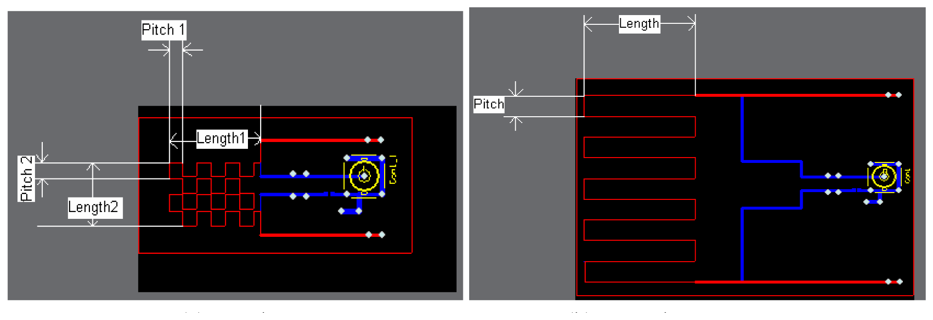
Figure 2.
Structure of the sensor.
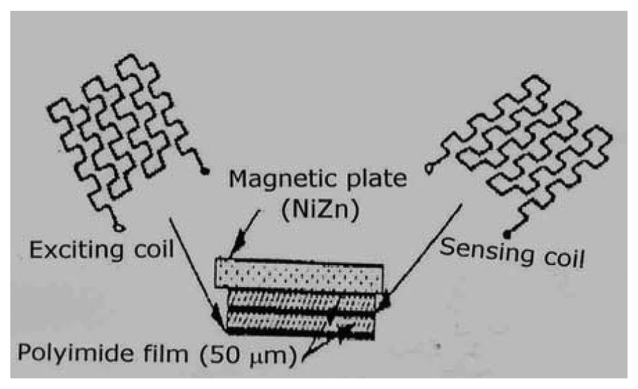
Figure 3.
Fabricated meander type sensors.
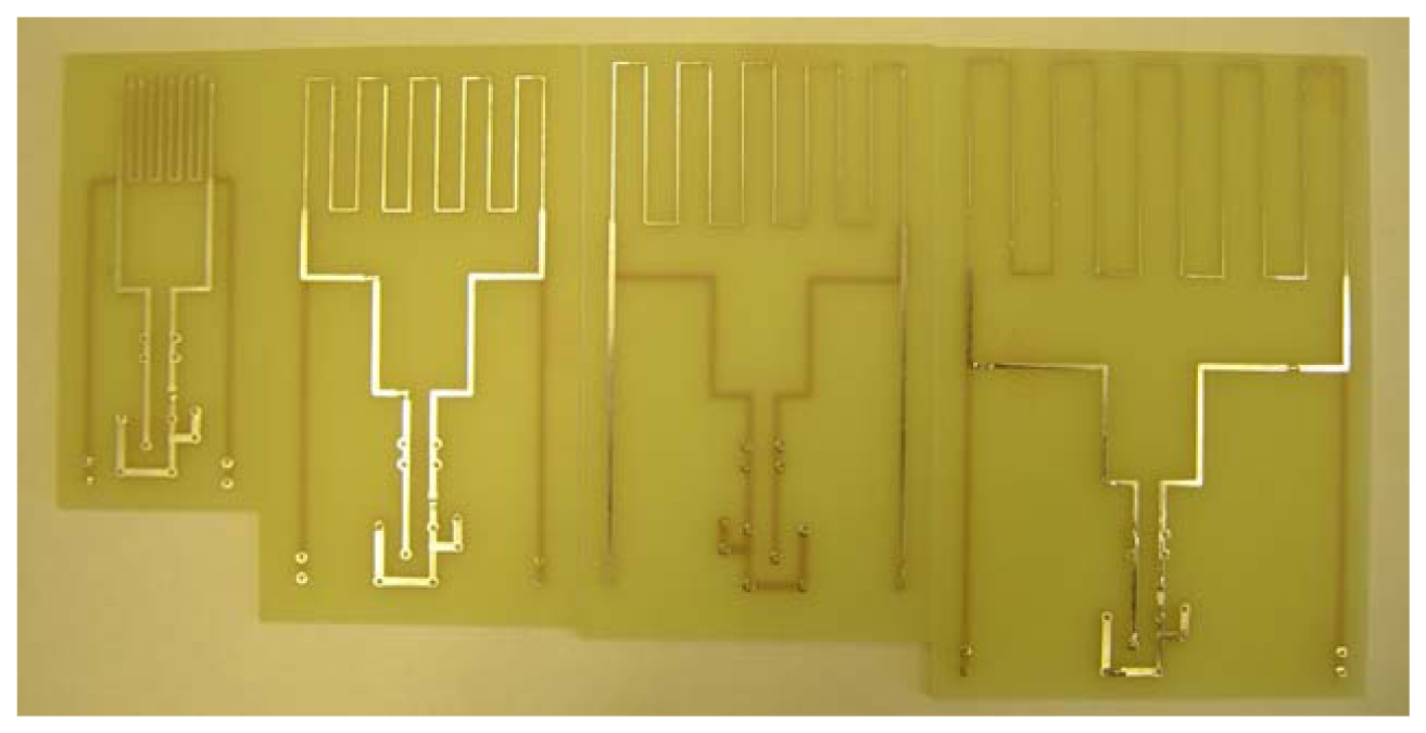
Figure 4.
Fabricated mesh type sensors.

Figure 5.
Operating principle of an interdigital sensor.

Figure 6.
Interdigital sensor structure, where the electrodes follow a finger-like or digit-like pattern.
Figure 6.
Interdigital sensor structure, where the electrodes follow a finger-like or digit-like pattern.

Figure 7.
Electric field formed between driven and ground electrodes for different wavelengths.

Figure 8.
Schematic diagram of interdigital type sensor.

Figure 9.
Fabricated interdigital type sensors.
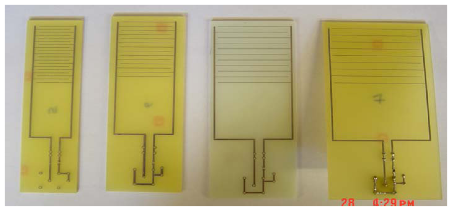
Figure 10.
Model of meander type sensor.
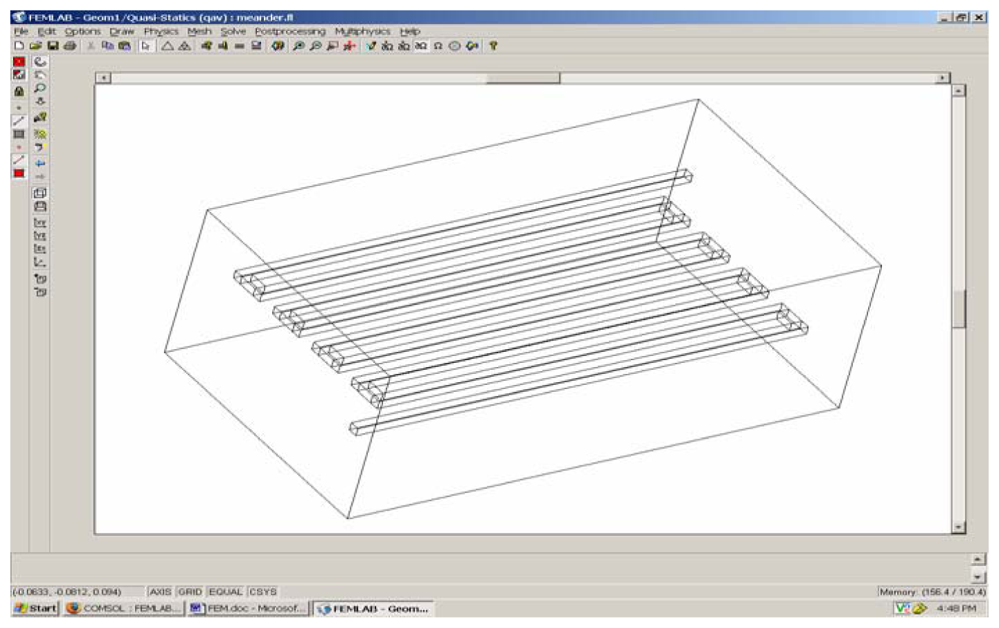
Figure 11.
Model after finite element mesh generation.

Figure 12.
Solved meander type sensor.
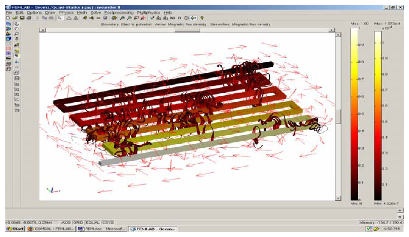
Figure 13.
Variation of reactance with frequency for meander sensor.
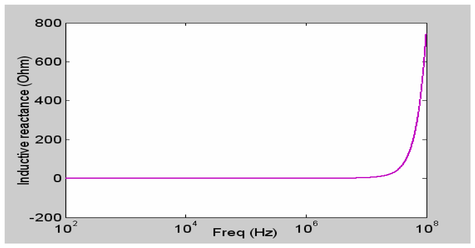
Figure 14.
Solution of mesh type sensor

Figure 15.
Variation of reactance with frequency for mesh sensor.
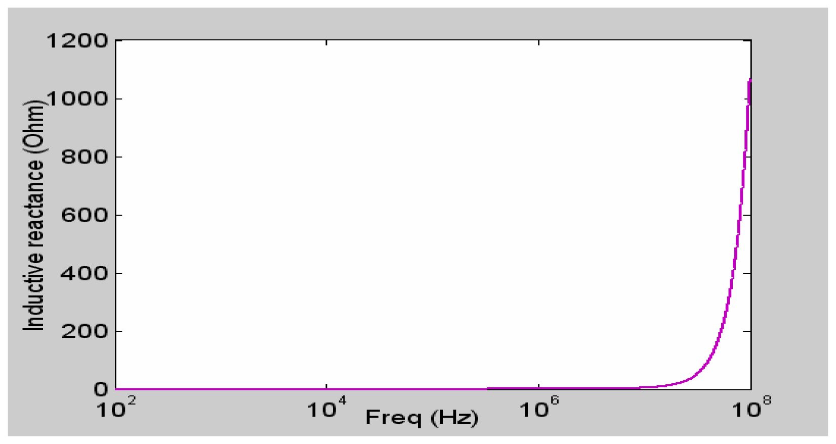
Figure 16.
Solution of interdigital type sensor.
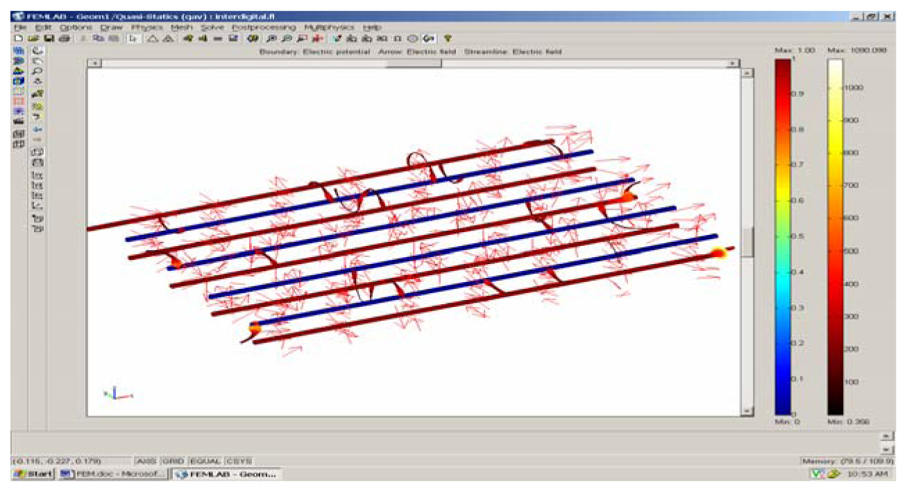
Figure 17.
Variation of reactance with frequency.

Figure 18.
Variation of the real part of transfer impedance with conductivity at 500 kHz for Mesh type sensor.
Figure 18.
Variation of the real part of transfer impedance with conductivity at 500 kHz for Mesh type sensor.
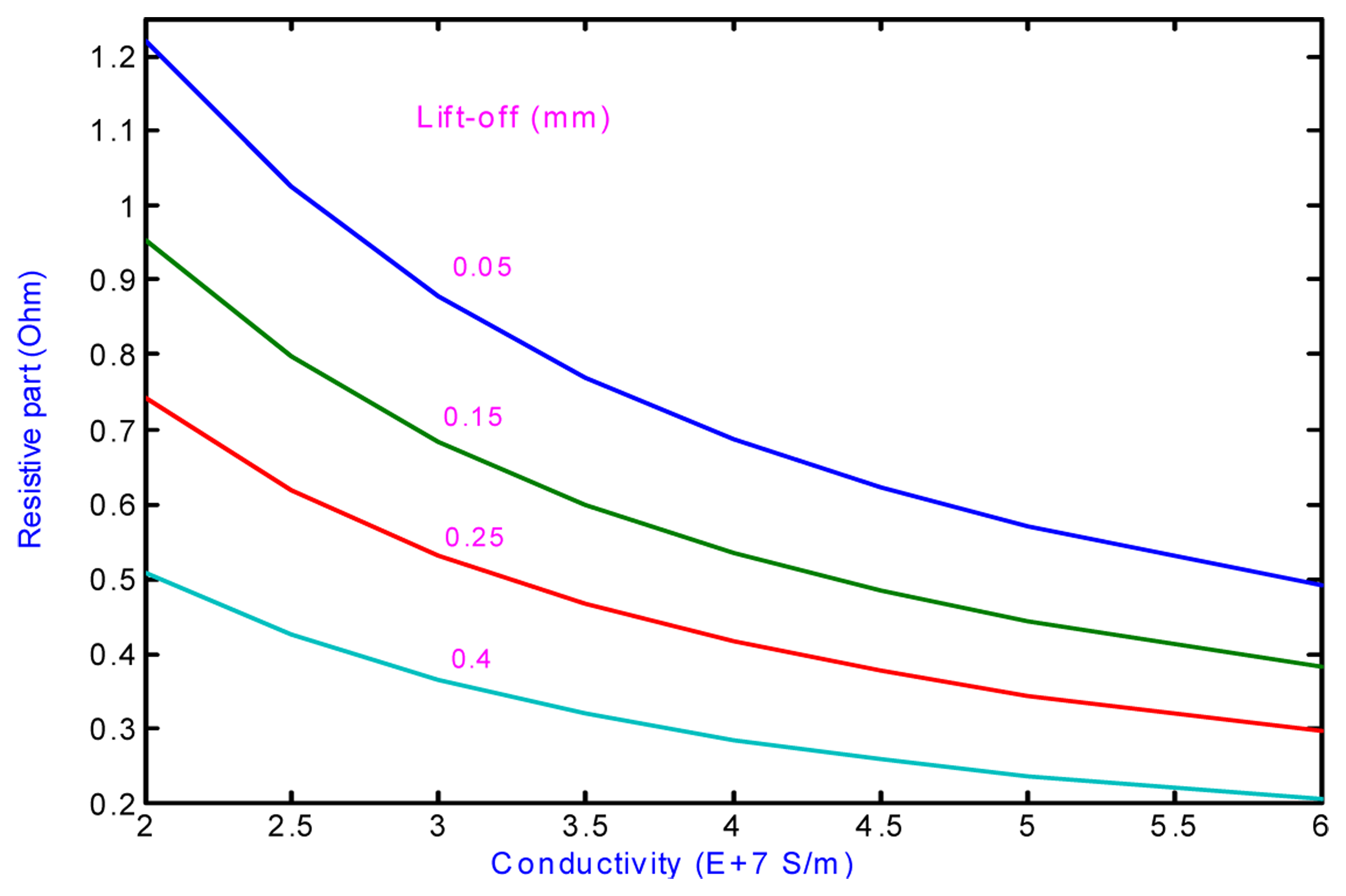
Figure 19.
Variation of the imaginary part of transfer impedance with conductivity at 500 kHz for Mesh type sensor.
Figure 19.
Variation of the imaginary part of transfer impedance with conductivity at 500 kHz for Mesh type sensor.
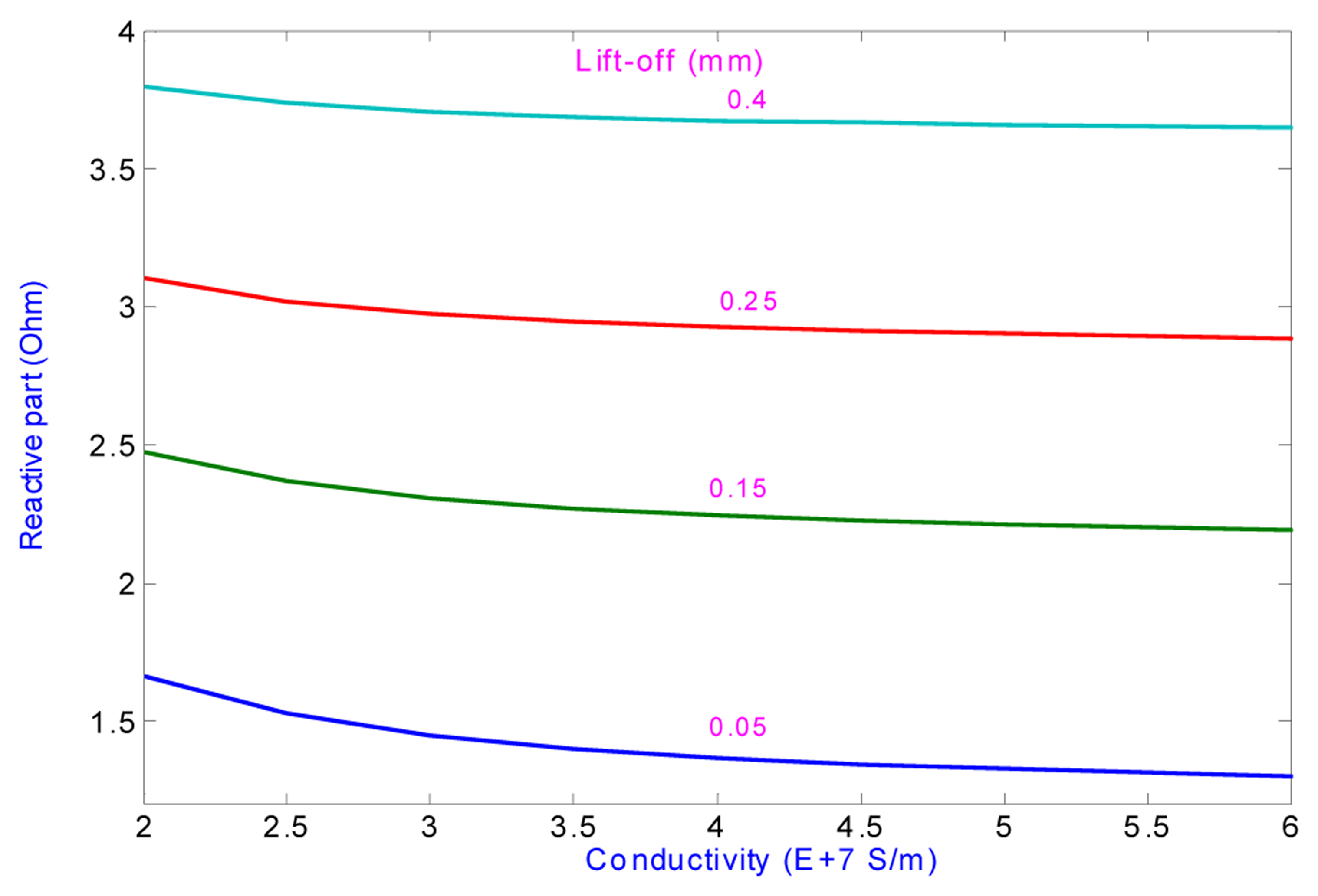
Figure 20.
Variation of the real part of transfer impedance with lift-off at 500 kHz.
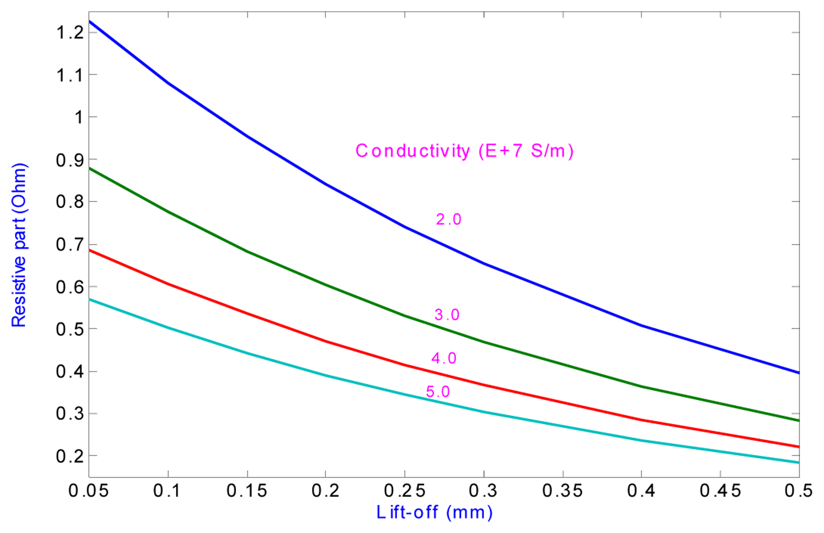
Figure 21.
Variation of the imaginary part of transfer impedance with lift-off at 500 kHz.

Figure 22.
Conductivity versus lift-off grid system obtained from finite element model.
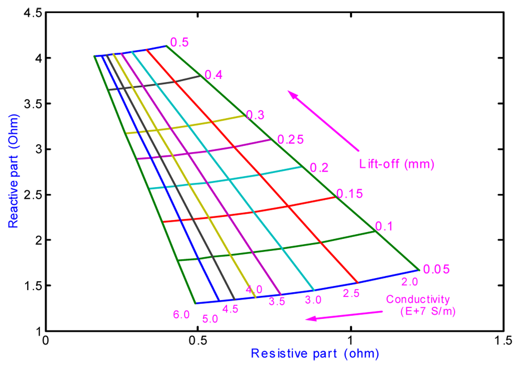
Figure 23.
The estimation of near-surface properties from the grid and measured data.
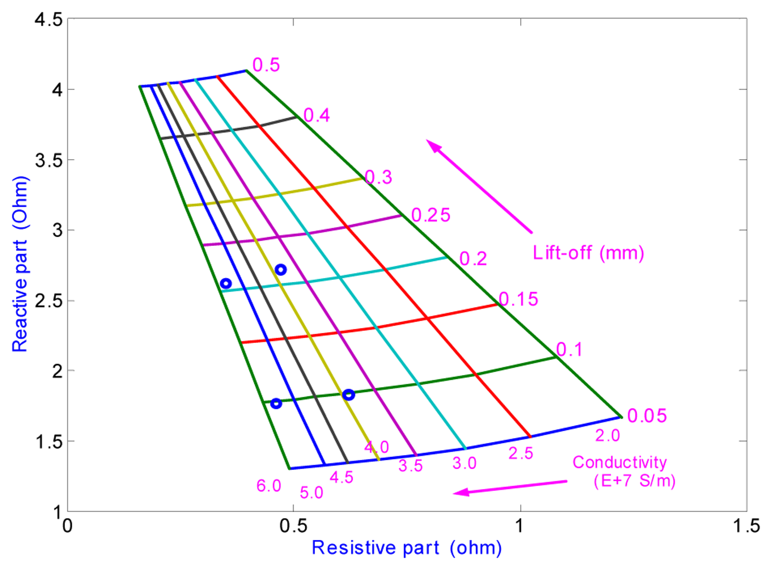
Figure 24.
Variation of skin-depth with frequency
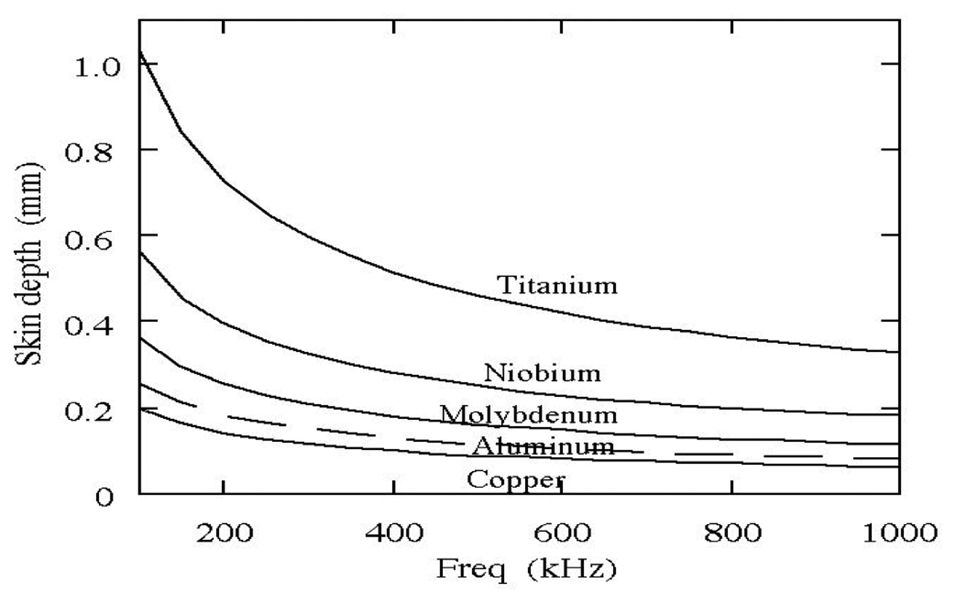
Figure 25.
The target PCB (PCB of Pentium processor).
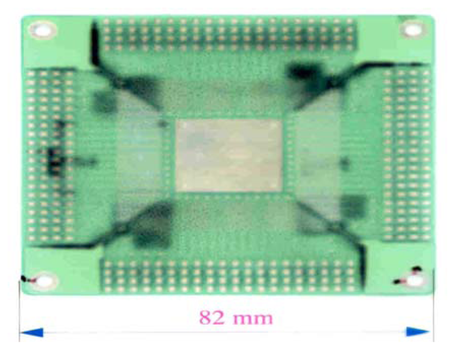
Figure 26.
The experimental set-up for PCB inspection.
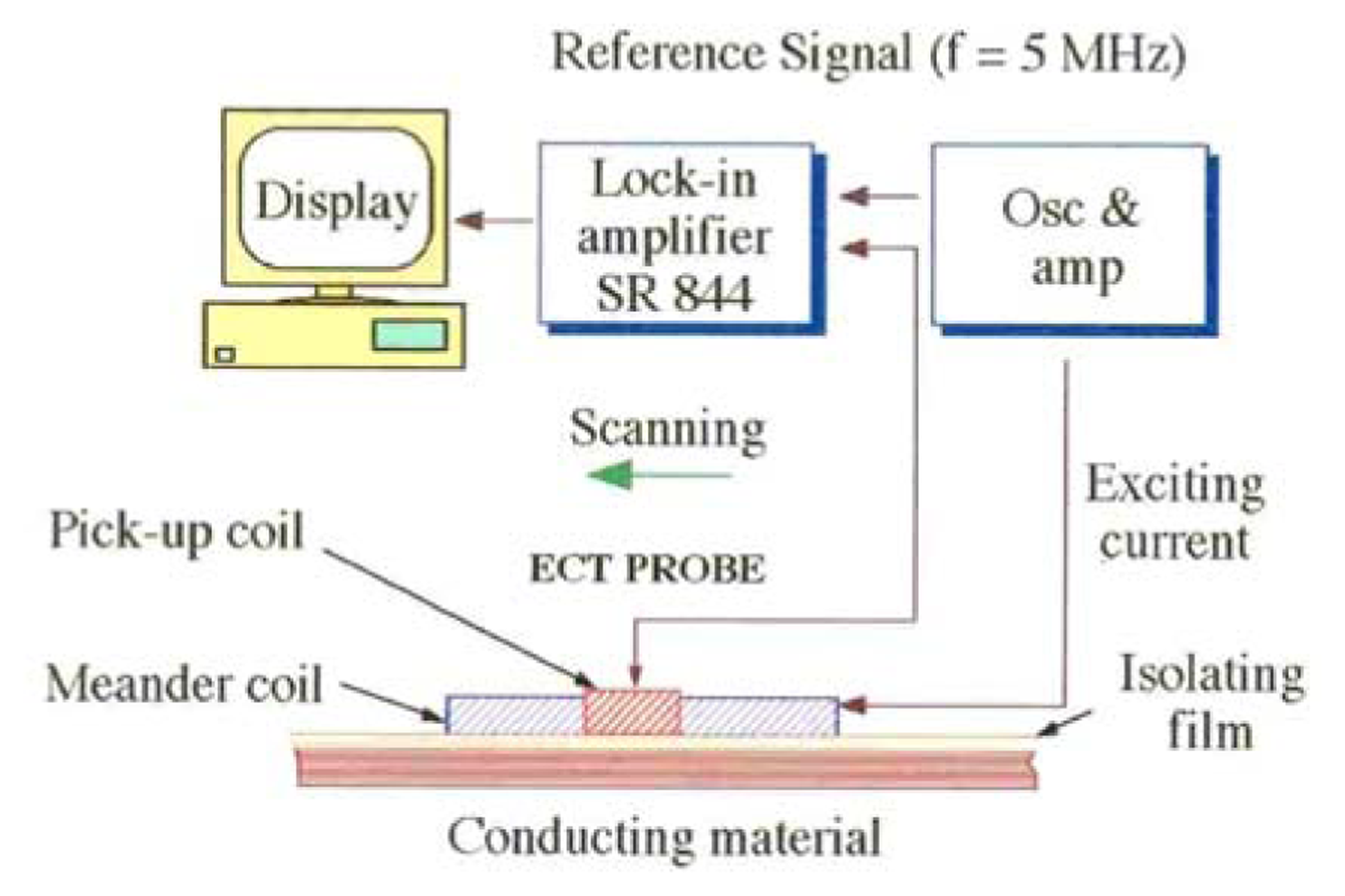
Figure 27.
Amplitude of the voltage across sensing coil with a defect in the PCB.
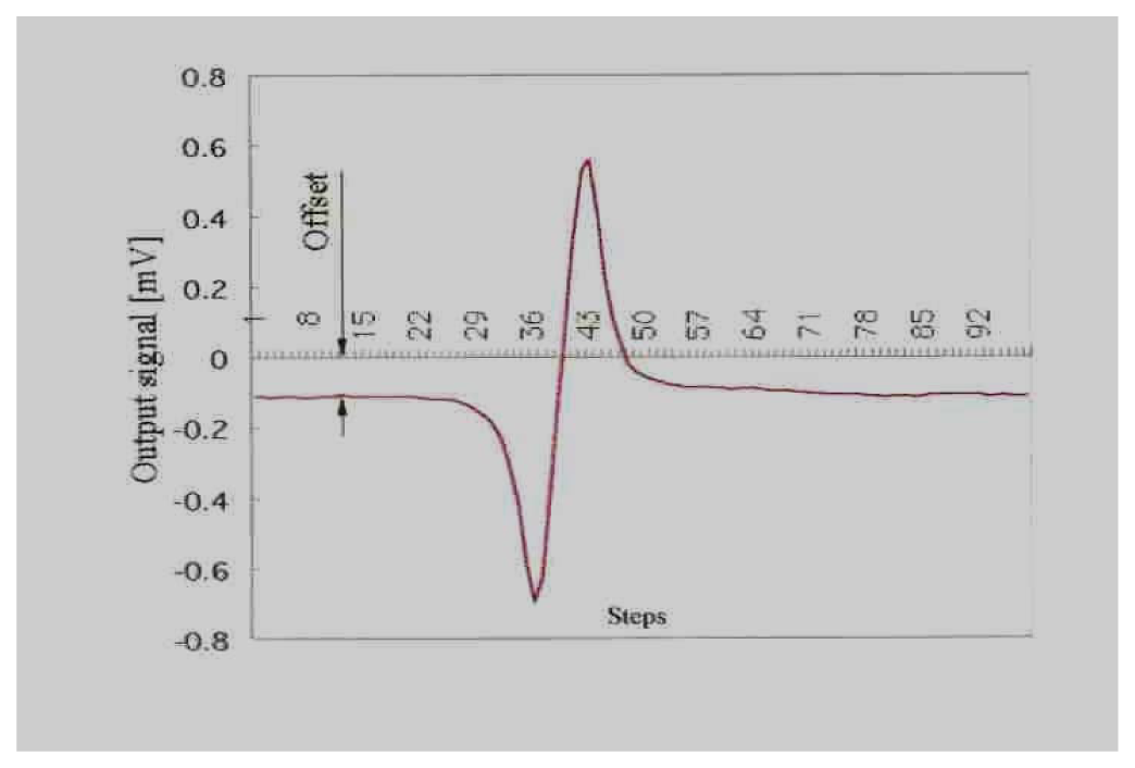
Figure 28.
Estimation of surface properties.
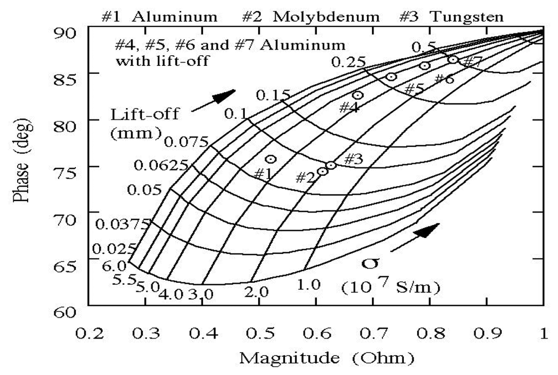
Figure 29.
Neural network aided property estimation.
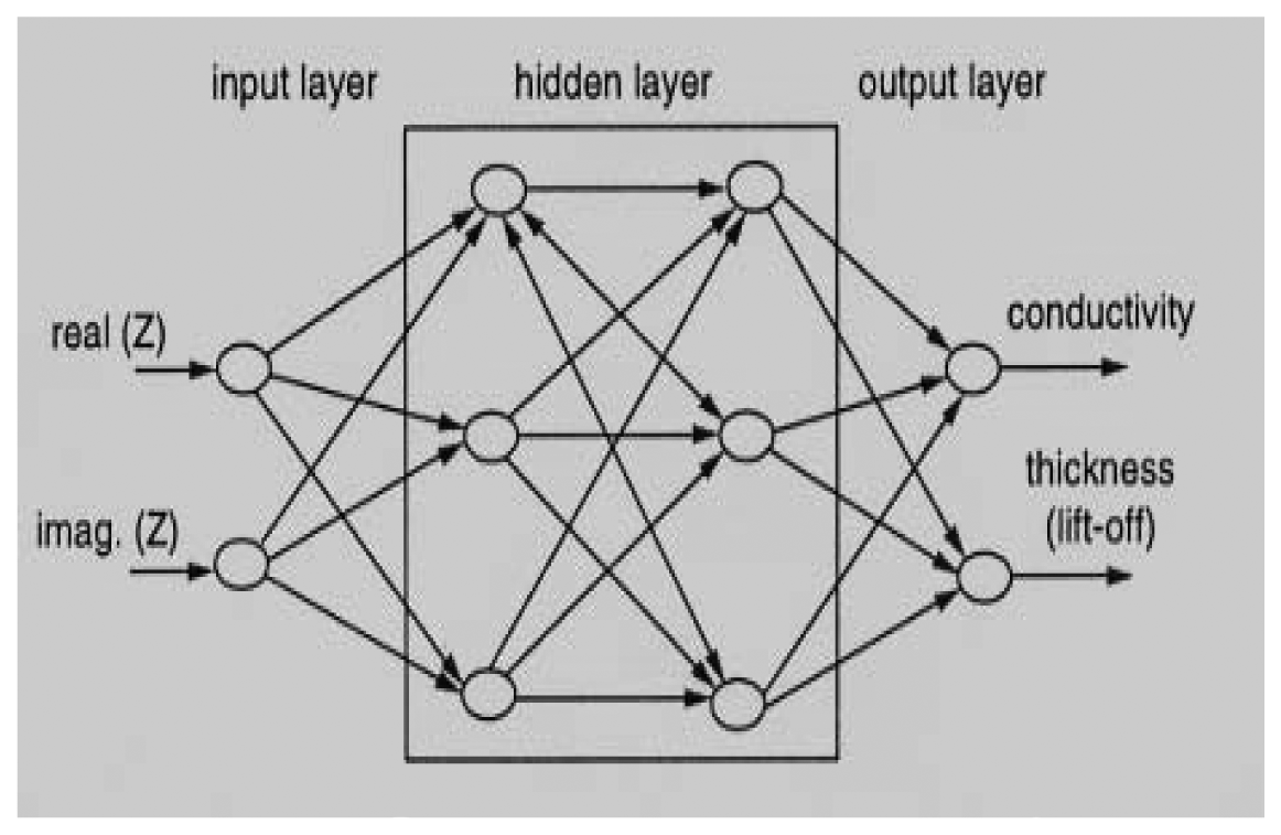
Figure 30.
The impedance magnitude as a function of frequency for different dielectric materials.
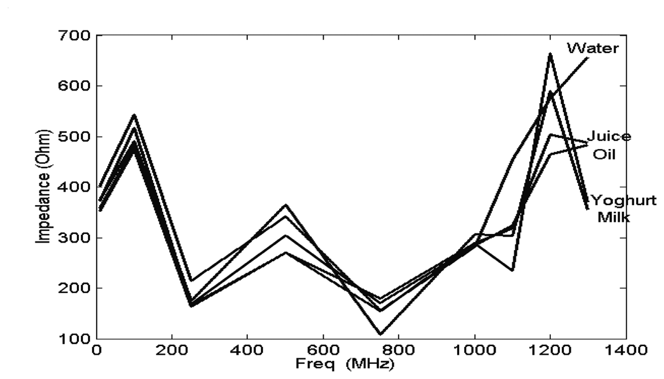
Figure 31.
The impedance magnitude as a function of frequency for milk with different lift-off.

Figure 32.
The impedance magnitude as a function of frequency for milk with different fat content at a lift-off of 5 mm.
Figure 32.
The impedance magnitude as a function of frequency for milk with different fat content at a lift-off of 5 mm.

Figure 33.
Variation of impedance with percentage of fat content at 750 MHz with 5 mm lift-off.

Figure 34.
Experimental setup for estimation of fat content in pork belly cuts.

Figure 35.
Pork belly sample dimensions.

Figure 36.
Sensor 1 characteristics for pork belly samples at orientation 1.
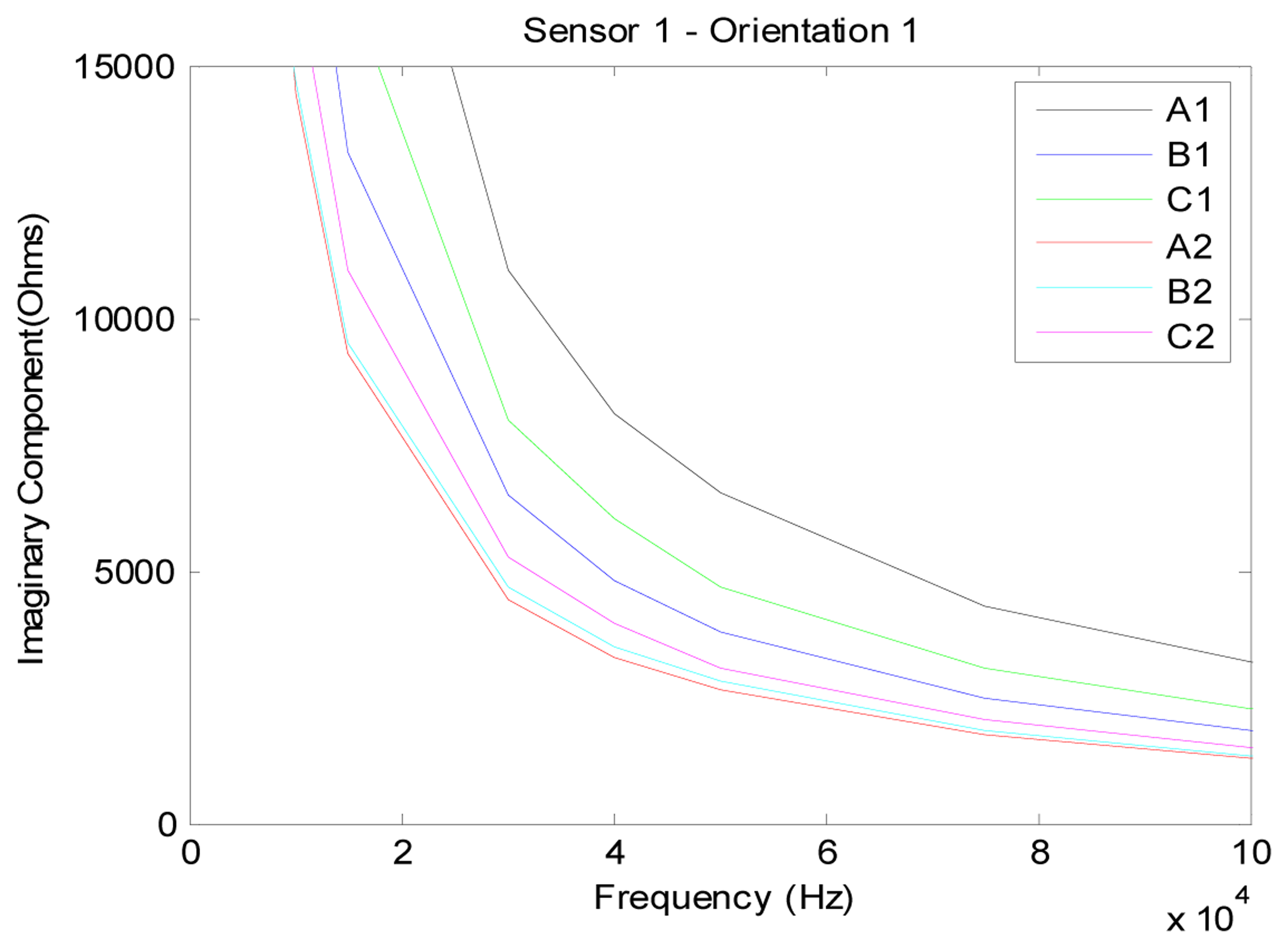
Figure 37.
Sensor 1 characteristics for pork belly samples at orientation 2.

Figure 38.
Sensor 1 characteristics for pork belly samples at orientation 3.

Figure 39.
Sensor 1 characteristics for pork belly samples at orientation 4.
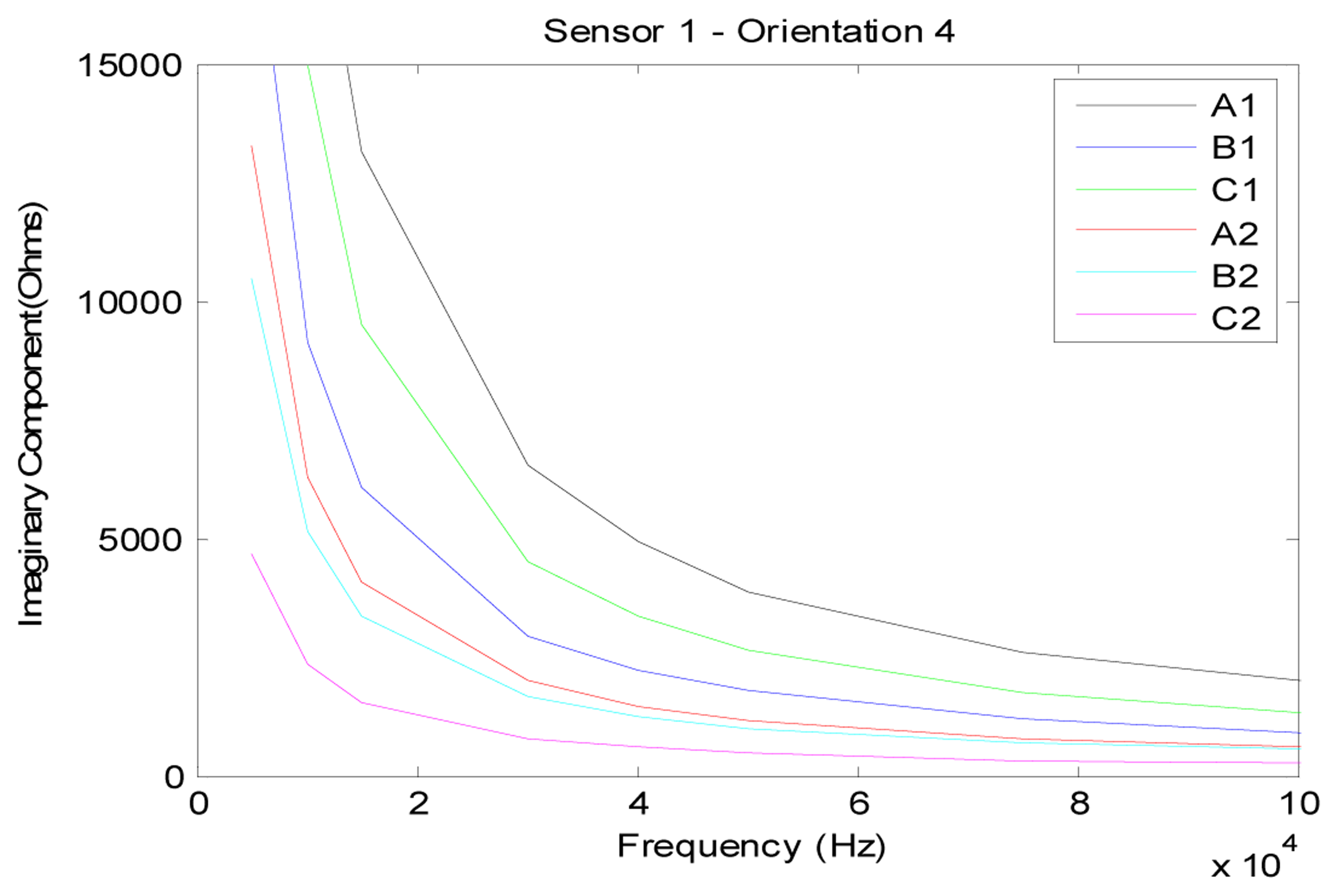
Figure 40.
Sensor 1 characteristics at 5 kHz for pork belly samples at orientation 1.

Figure 41.
Sensor 1 characteristics at 5 kHz for pork belly samples at orientation 2.
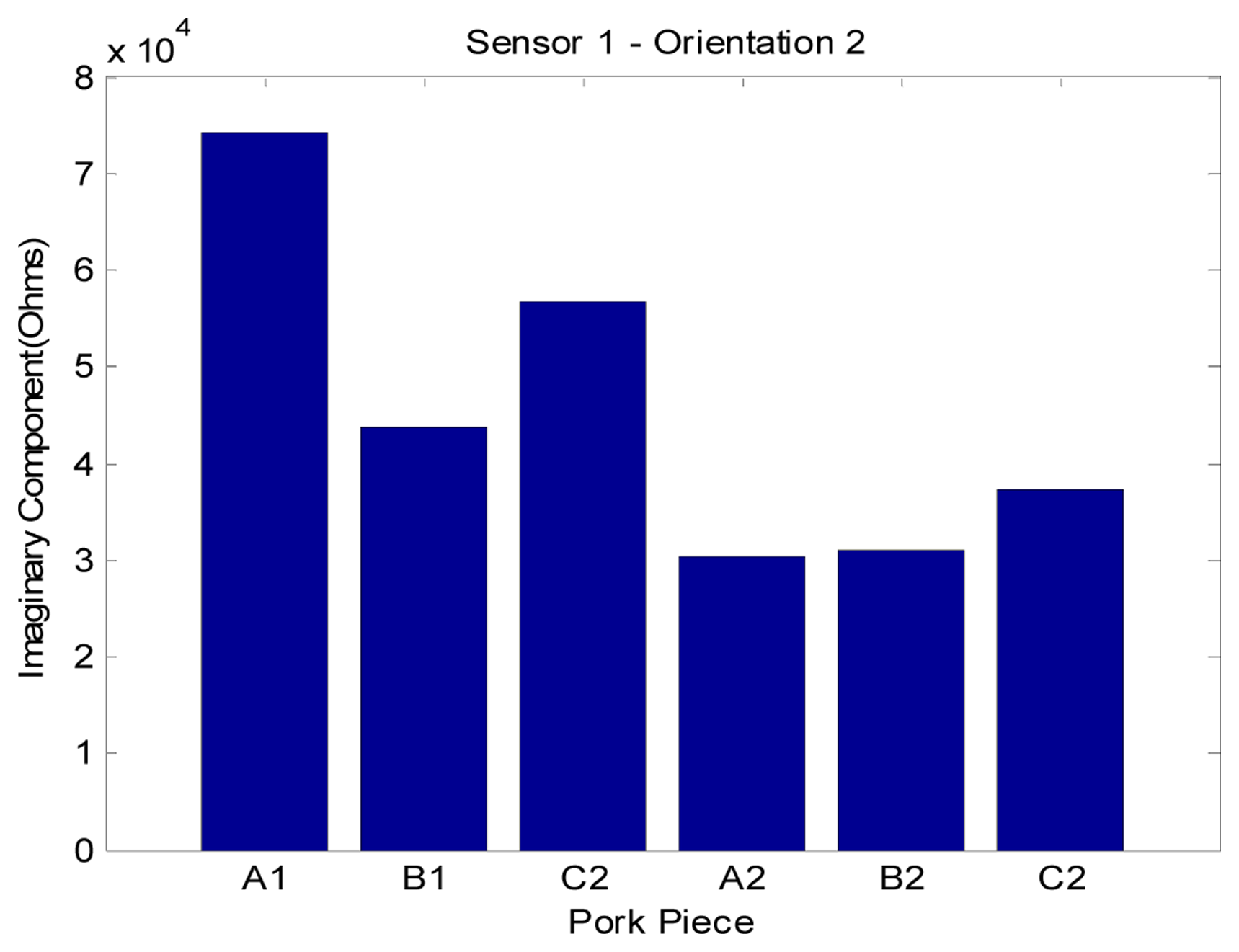
Figure 42.
Sensor 1 characteristics at 5 kHz for pork belly samples at orientation 3.

Figure 43.
Sensor 1 characteristics at 5 kHz for pork belly samples at orientation 4.


| Sensor | Pitch (mm) | Length (mm) |
|---|---|---|
| 1 | 2 | 20 |
| 2 | 5 | 25 |
| 3 | 6 | 30 |
| 4 | 8 | 40 |
| Sensor | Pitch 1 (mm) | Pitch 2 (mm) | Length 1 (mm) | Length 2 (mm) |
|---|---|---|---|---|
| 1 | 2 | 2.5 | 10 | 10 |
| 2 | 3 | 3.5 | 14 | 14 |
| 3 | 3 | 3.5 | 20 | 14 |
| 4 | 4 | 5 | 27 | 18 |
| Sensor | Wavelength, λ (mm) | Length (mm) |
|---|---|---|
| 1 | 5 | 20 |
| 2 | 6 | 30 |
| 3 | 8 | 40 |
| 4 | 10 | 50 |
| Conductivity of Aluminum | From Grid System (S/m) | Neural Network Model (S/m) |
|---|---|---|
| With No lift-off | 3.6 E+7 | 3.53 E+7 |
| With 0.1 mm lift-off | 3.7 E+7 | 3.54 E+7 |
| With 0.2 mm lift-off | 3.8 E+7 | 3.53 E+7 |
| With 0.3 mm lift-off | 3.8 E+7 | 3.51 E+7 |
| With 0.4 mm lift-off | 3.4 E+7 | 3.49 E+7 |
| Sensor | Periodicity(cm) | Finger-length(cm) |
|---|---|---|
| 1 | 15 | 120 |
| 2 | 20 | 120 |
| 3 | 30 | 120 |
| Chemical Test | Sample A1 | Sample A2 | Sample B2 |
|---|---|---|---|
| 30.09 | 19.96 | 17.36 |
| Sample | Effective Permittivity (εeff) | Parameter of Index (Қ) |
|---|---|---|
| Orientation 1 | ||
| A1 | 2.7871 | 0.3588 |
| B1 | 4.7246 | 0.2117 |
| C1 | 3.6407 | 0.2747 |
| A2 | 6.1203 | 0.1634 |
| B2 | 6.0075 | 0.1665 |
| C2 | 4.9867 | 0.2005 |
| Orientation 2 | ||
| A1 | 2.7871 | 0.3588 |
| B1 | 4.7246 | 0.2117 |
| C1 | 3.6407 | 0.2747 |
| A2 | 6.1203 | 0.1634 |
| B2 | 6.0075 | 0.1665 |
| C2 | 4.9867 | 0.2005 |
| Orientation 3 | ||
| A1 | 4.9093 | 0.2037 |
| B1 | 10.8659 | 0.0920 |
| C1 | 6.2759 | 0.1593 |
| A2 | 14.0014 | 0.0714 |
| B2 | 17.7739 | 0.0563 |
| C2 | 40.1206 | 0.0249 |
| Orientation 4 | ||
| A1 | 4.9093 | 0.2037 |
| B1 | 10.8659 | 0.0920 |
| C1 | 6.2759 | 0.1593 |
| A2 | 14.0014 | 0.0714 |
| B2 | 17.7739 | 0.0563 |
| C2 | 40.1206 | 0.0249 |
| Sample | Parameter of Index (Қ) | Calculated Fat content | Calculated protein content |
|---|---|---|---|
| A1 | 0.3987 | 30.06 | 12.49 |
| A2 | 0.1633 | 18.74 | 16.28 |
| B1 | 0.2353 | 22.20 | 15.12 |
| B2 | 0.1644 | 18.80 | 16.26 |
| C1 | 0.3053 | 25.57 | 13.99 |
| C2 | 0.2005 | 20.53 | 15.68 |
© 2005 by MDPI ( http://www.mdpi.org). Reproduction is permitted for noncommercial purposes.
Share and Cite
MDPI and ACS Style
Mukhopadhyay, S.C. Novel Planar Electromagnetic Sensors: Modeling and Performance Evaluation. Sensors 2005, 5, 546-579. https://doi.org/10.3390/s5120546
AMA Style
Mukhopadhyay SC. Novel Planar Electromagnetic Sensors: Modeling and Performance Evaluation. Sensors. 2005; 5(12):546-579. https://doi.org/10.3390/s5120546
Chicago/Turabian StyleMukhopadhyay, Subhas C. 2005. "Novel Planar Electromagnetic Sensors: Modeling and Performance Evaluation" Sensors 5, no. 12: 546-579. https://doi.org/10.3390/s5120546