Fast and Automatic Reconstruction of Semantically Rich 3D Indoor Maps from Low-quality RGB-D Sequences

 ,
,  ,
,
Abstract
:1. Introduction
2. Related Work
3. Methodology
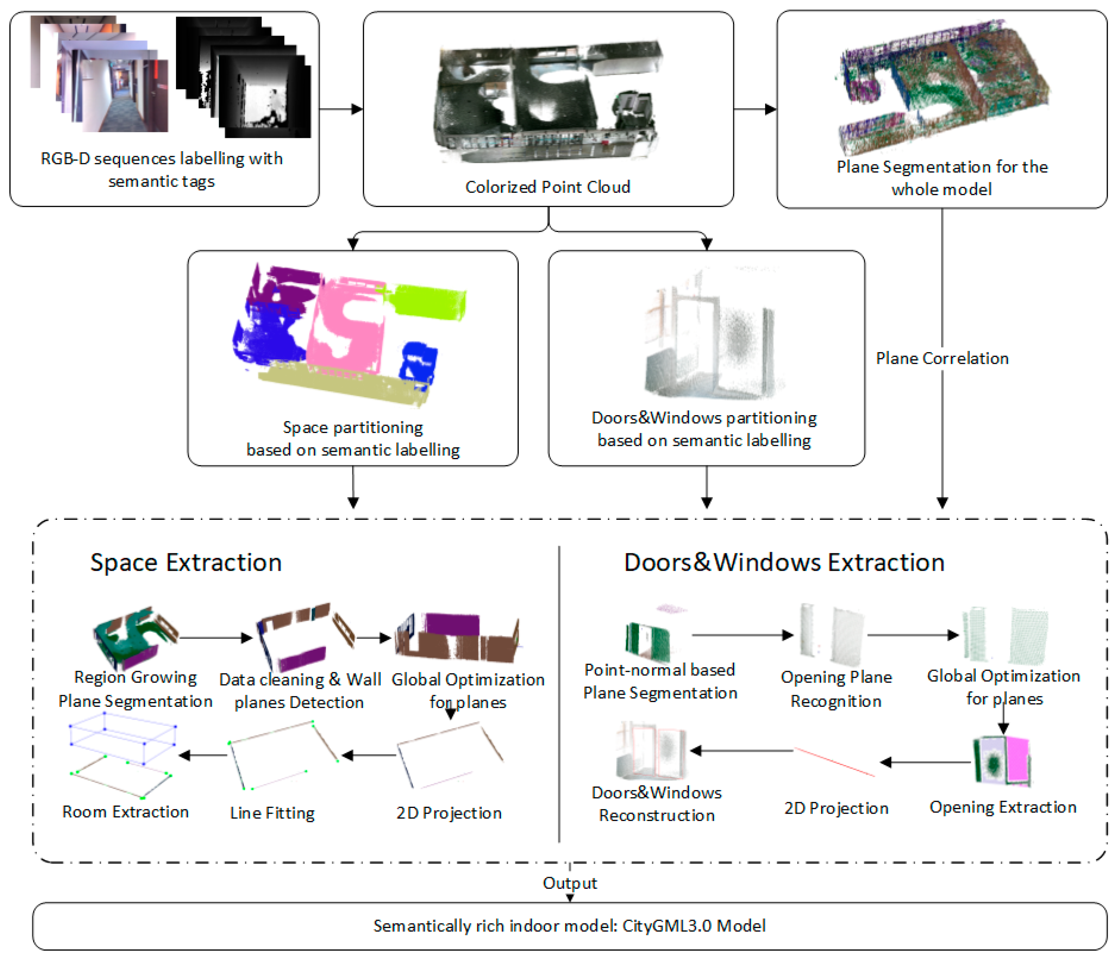
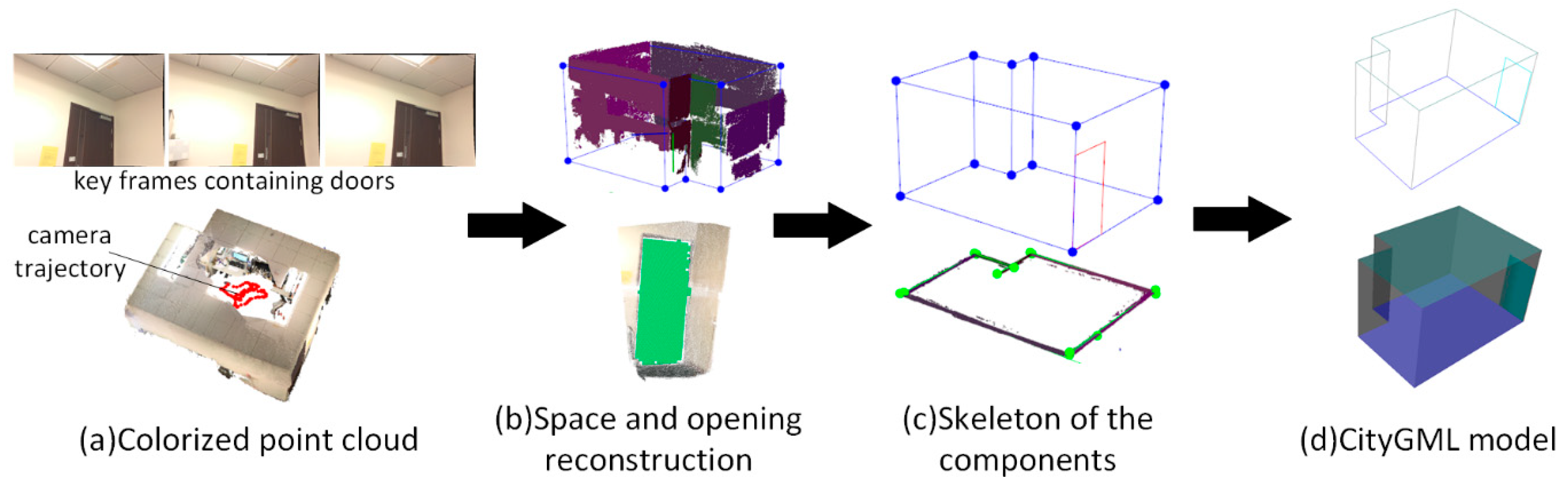
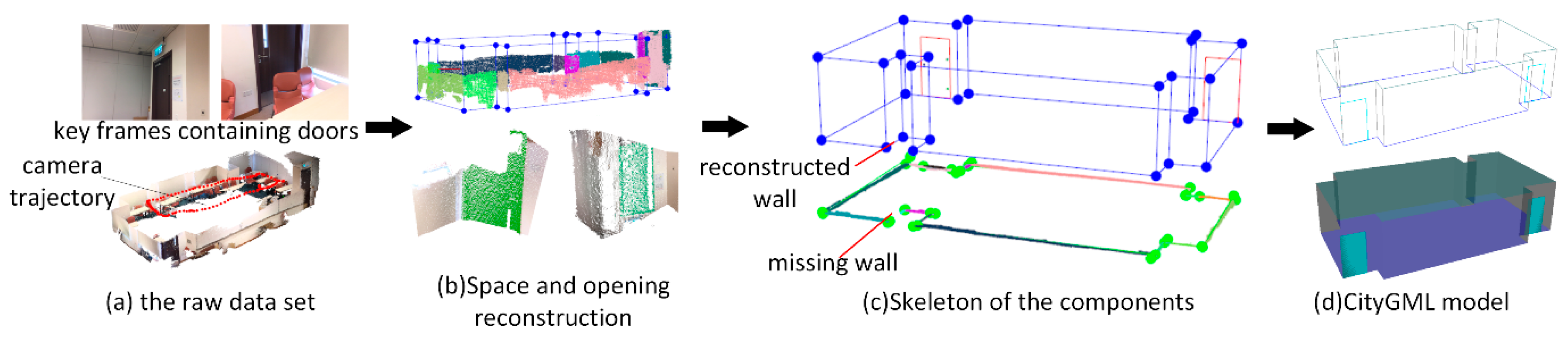
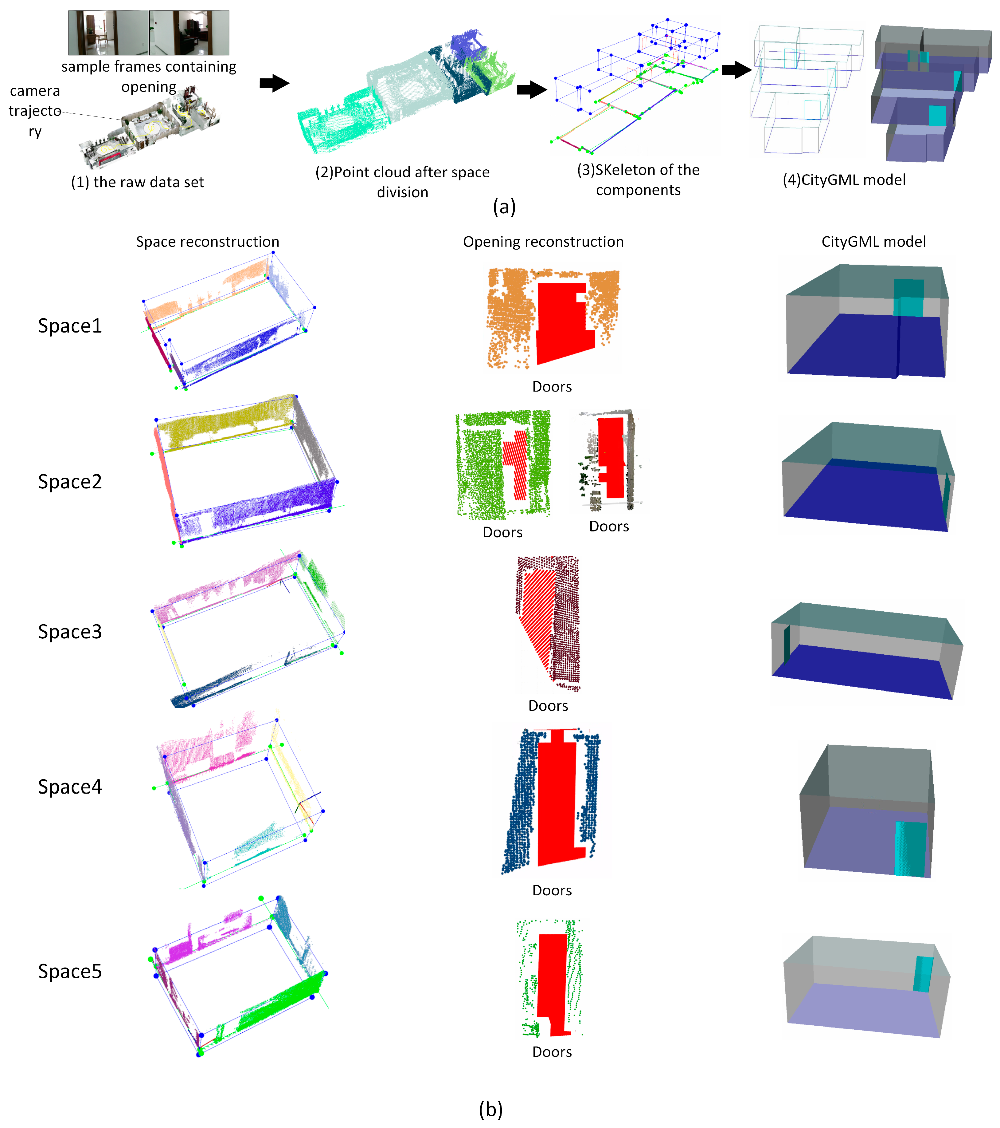
3.1. Overview
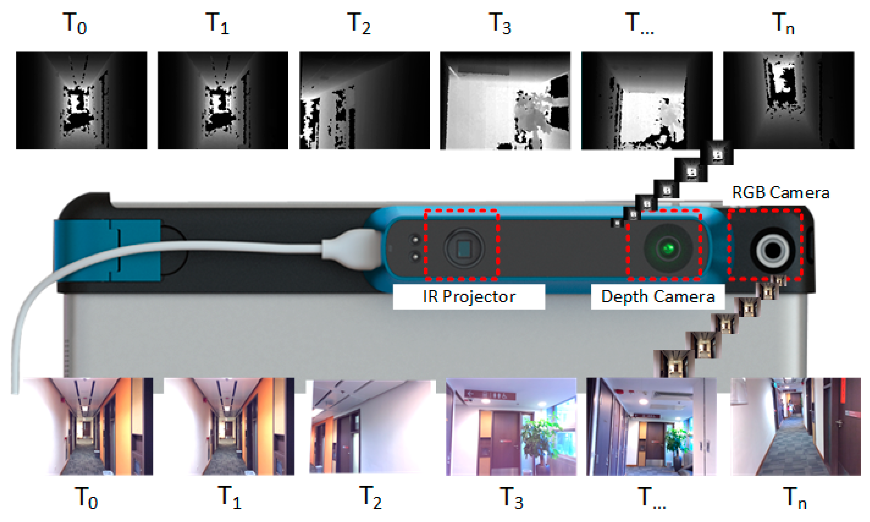
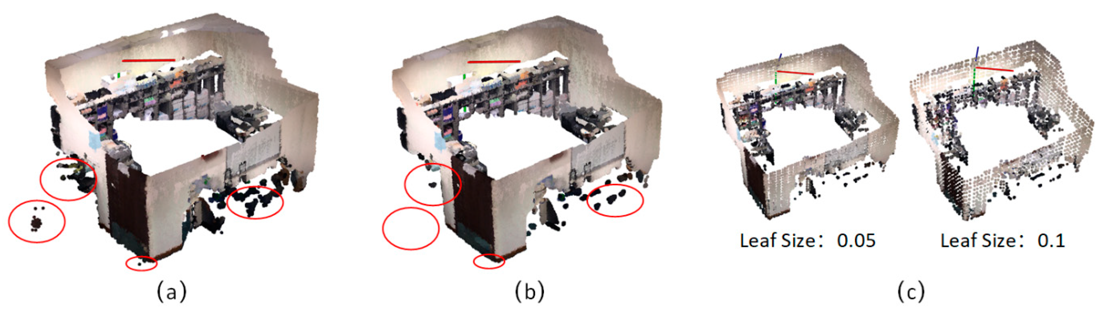
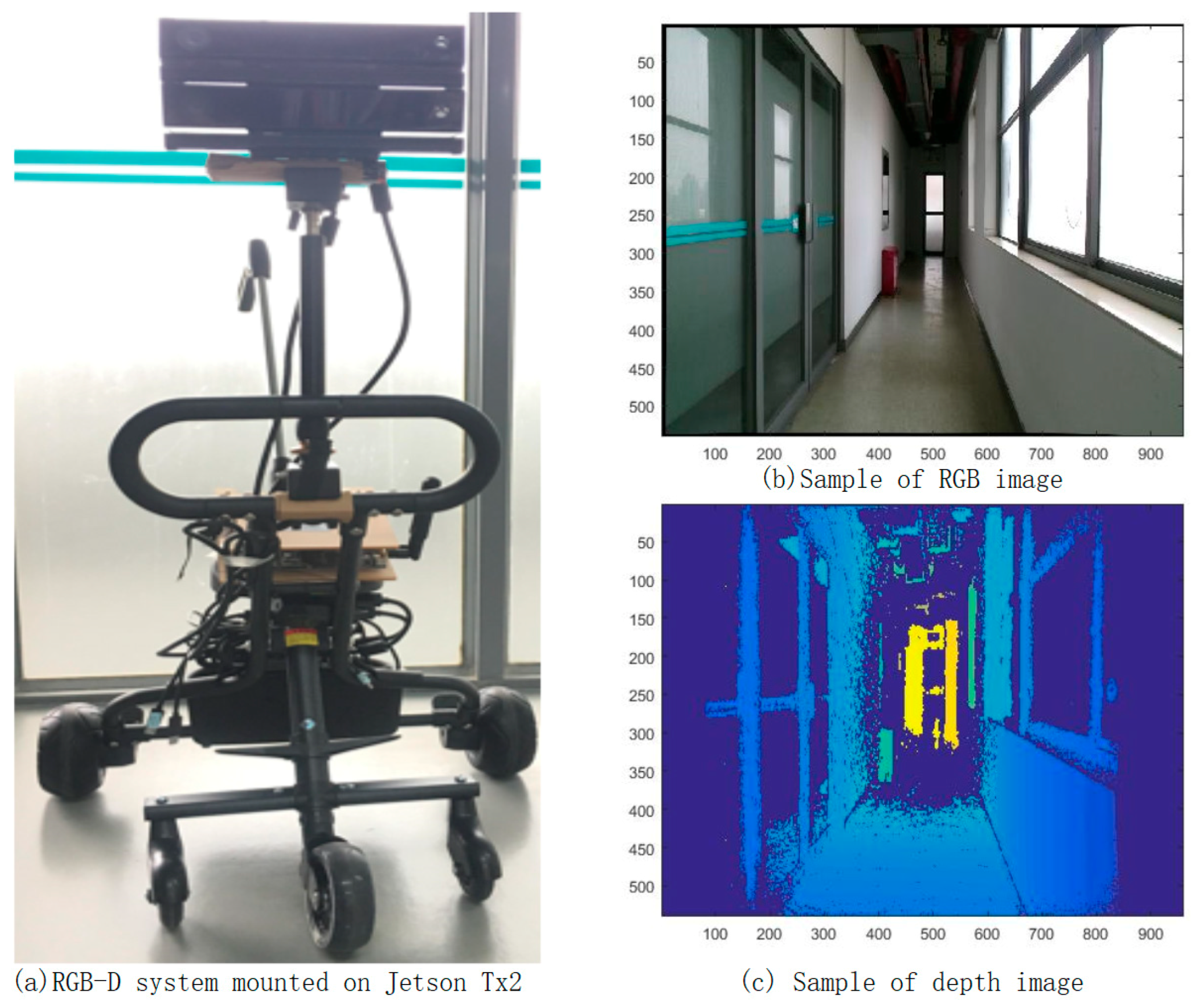
3.2. Data Pre-Processing
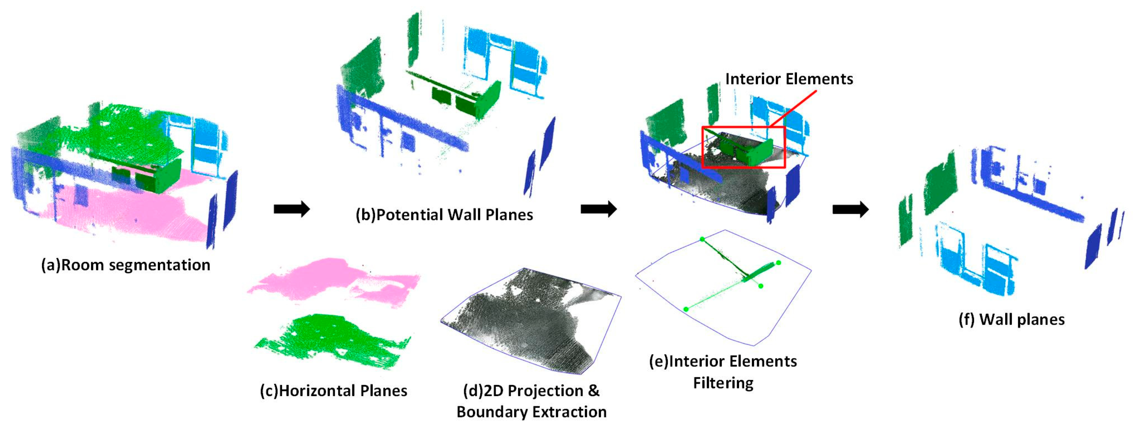
3.3. Spaces Division and Extraction
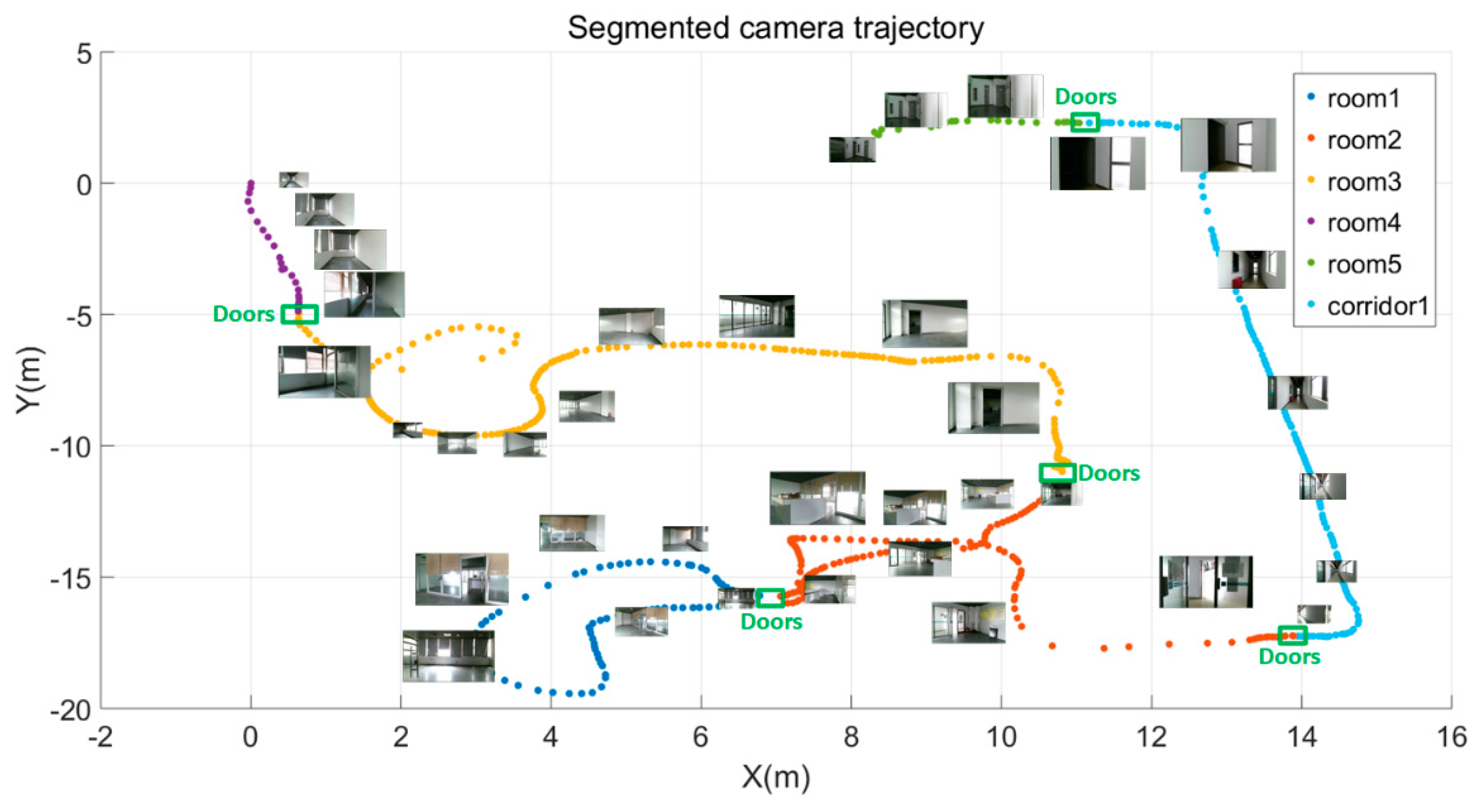
3.3.1. Spaces Partition
3.3.2. Generation of Wall Candidates
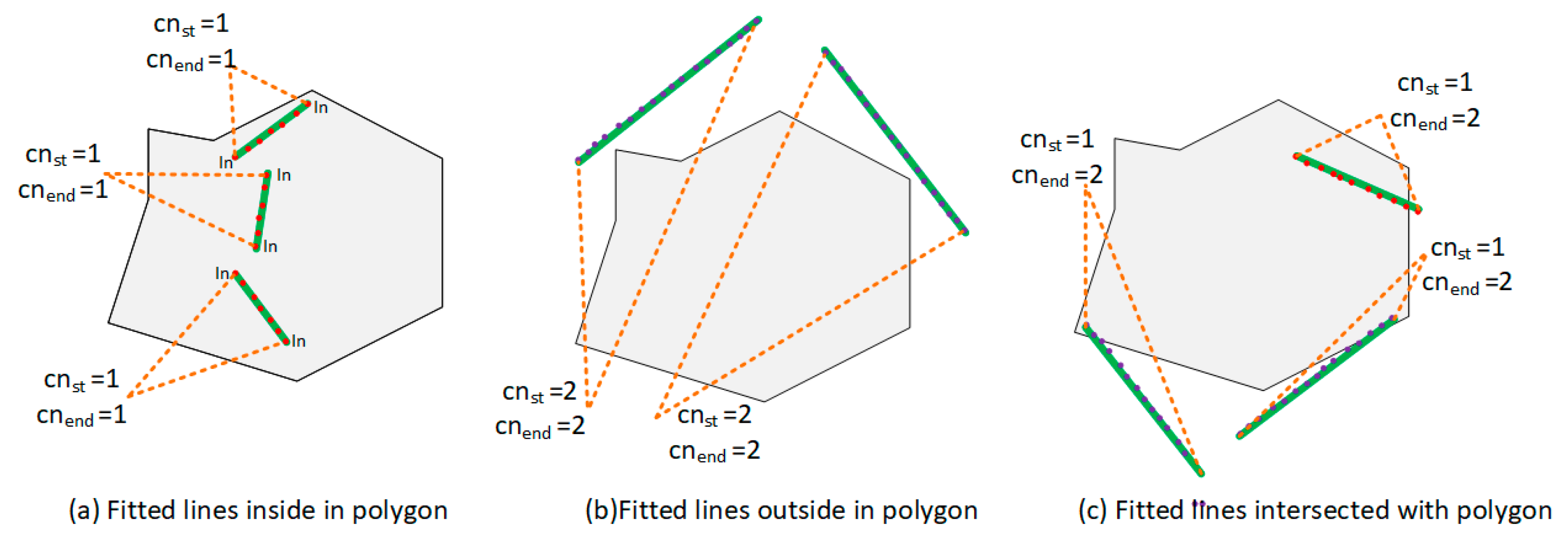
| Algorithm 1: Interior elements filtering algorithm |
| Input: Projected potential wall planes: 2D polygon consist of points: Percentage threshold of length in interior and external of polygon: Line fitting function based RANSAC method: Fitted line: Distance calculation function: Distance from endpoints to intersection point: Intersection function of two line segments: Intersection point of two line segments: Crossing number function to determine the inclusion of a point in a 2D polygon: Crossing number from a ray of endpoint to the polygon boundary edges: |
| Output: index of interior planes: ; index of wall planes: ; |
| 1. 2. While is not empty do 3. , 4. Do line fitting for 5. 6. Detection the crossing number of the ray from the endpoint and the polygon boundary 7. , 8. If is odd && is odd then 9. 10. else if is even && is even then 11. 12. else 13. Do intersection for the fitted line and the polygon boundary 14. 15. Calculate the distance between endpoints () and 16. , 17. if ( is even && ) || ( is even && ) then 18. 19. else 20. 21. end if 22. end if 23. end while 24. Return , |
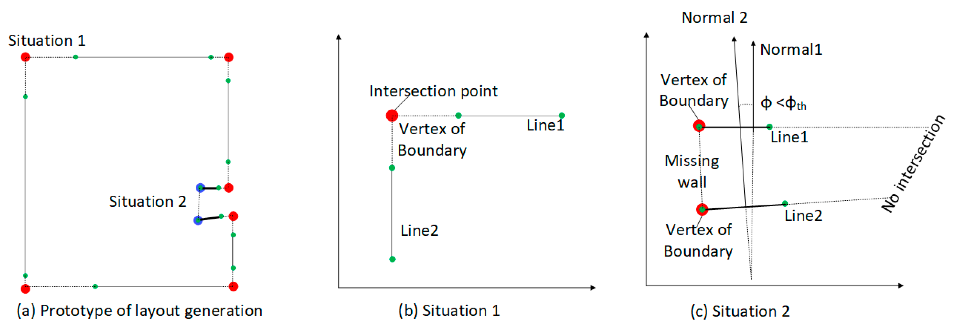
3.3.3. Determination of Space Layout and Parameterization
| Algorithm 2: Boundary generation algorithm |
| Input: Projected wall planes: Fitted lines vector: = Line fitting function based RANSAC method: Minimum Distance calculation between the current point and others function: Enum of the endpoints of line: Map of Index of Nearest Neighbors of the fitted lines and the endpoints of the target line: Index of the lines by order: Intersection function of two line segments: Angle calculation of two line function: Angle threshold: |
| Output: Vertex of space boundary: |
| 1. ,, 2. for i = 0 to size () do 3. Do line fitting for 4. 5. end for 6. for i = 0 to size () do 7. Calculate minimum distance between the endpoint and others and output the index of nearest neighbor. 8. , 9. end for 10. Set the first line as start line: 11. for i = 0 to size () do 12. if equal to 0 13. 14. else 15. ) 16. if don’t contains 17. Then 18. 19. Calculate the intersection point of two adjacent line and add to points of space boundary 20. 21. If the angle is less than 22. , , 23. else 24. 25. break 26. end if 27. if is equal to 0 28. break 29. end if 30. end for 31. Return |
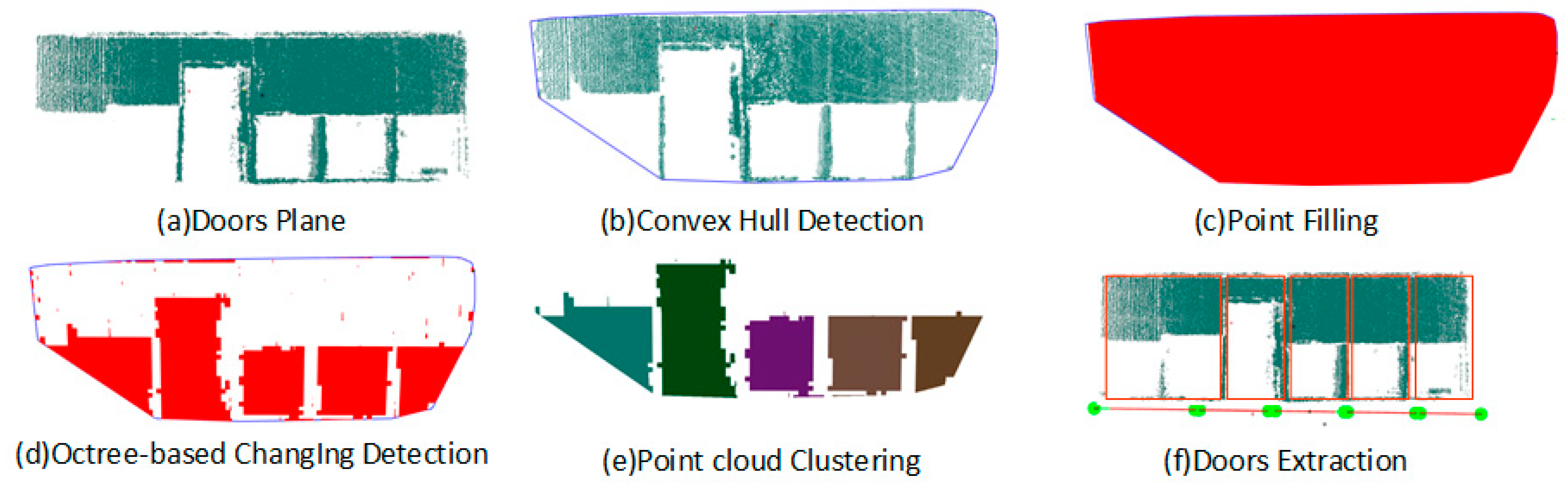
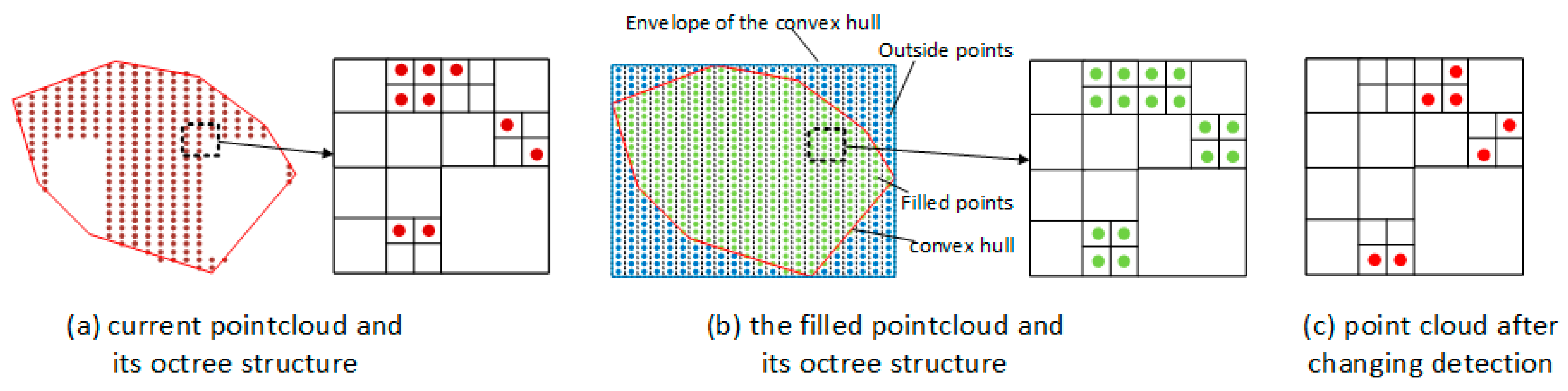
3.4. Opening Extraction
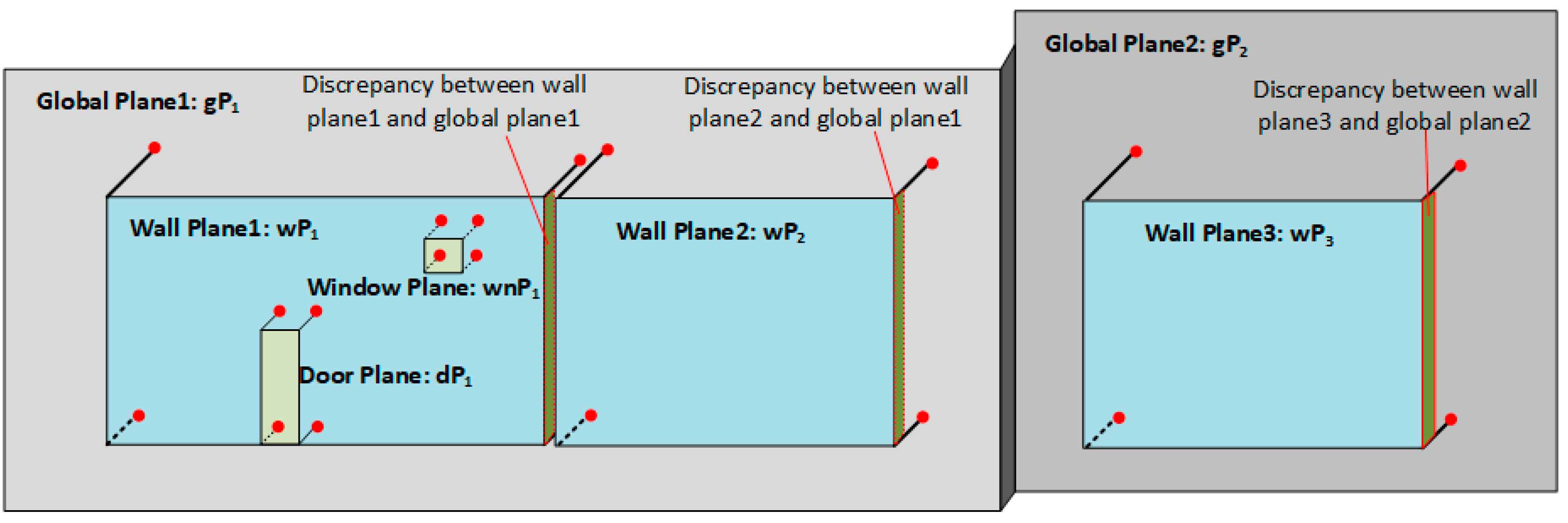
3.5. Global Optimization for Planes
4. Experimental Results and Discussion
5. Conclusions
- Benefiting from the multiple types of data set and the advantage of interactive data collection of the RGB-D mapping system, the proposed method provides new opportunities to use low-quality RGB-D sequences to reconstruct semantically rich 3D indoor models that include wall, opening, ceiling, and floor components.
- For point cloud data with significant occlusion, most components can be recognized correctly to achieve an average accuracy of 97.73%. Some components in case study (2) and case study (3) that are absent from the point cloud can be recalled based on the layout determination algorithm. The reconstruction results indicate the robustness of the proposed methodology for low-quality point clouds.
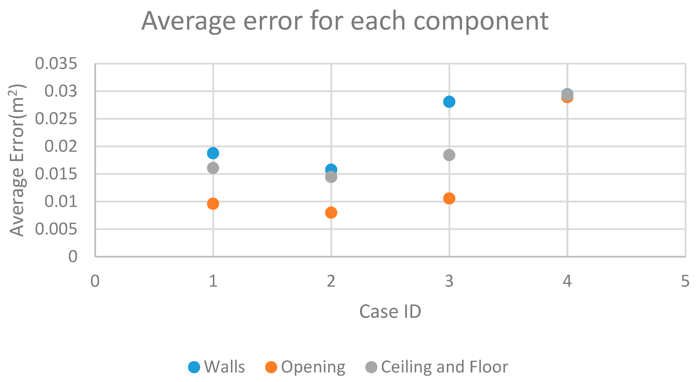
- The proposed reconstruction method produces an area dimension error within 3% for all cases. The measurement results indicate that modeling accuracy can be affected by the range sizes of the components. Higher range sizes result in lower accuracy.
Author Contributions
Funding
Conflicts of Interest
References
- Wang, C.; Cho, Y.K.; Kim, C. Automatic BIM component extraction from point clouds of existing buildings for sustainability applications. Autom. Constr. 2015, 56, 1–13. [Google Scholar] [CrossRef]
- Xiong, X.; Adan, A.; Akinci, B.; Huber, D. Automatic creation of semantically rich 3D building models from laser scanner data. Autom. Constr. 2013, 31, 325–337. [Google Scholar] [CrossRef] [Green Version]
- Furukawa, Y.; Curless, B.; Seitz, S.M.; Szeliski, R. Reconstructing building interiors from images. In Proceedings of the 2009 IEEE 12th International Conference on Computer Vision, Kyoto, Japan, 29 September–2 October 2009; pp. 80–87. [Google Scholar]
- Tang, P.; Huber, D.; Akinci, B.; Lipman, R.; Lytle, A. Automatic reconstruction of as-built building information models from laser-scanned point clouds: A review of related techniques. Autom. Constr. 2010, 19, 829–843. [Google Scholar] [CrossRef]
- Turner, E.; Zakhor, A. Floor plan generation and room labeling of indoor environments from laser range data. In Proceedings of the 2014 International Conference on Computer Graphics Theory and Applications (GRAPP), Lisbon, Portugal, 5–8 January 2014; pp. 1–12. [Google Scholar]
- Darwish, W.; Tang, S.; Li, W.; Chen, W. A New Calibration Method for Commercial RGB-D Sensors. Sensors 2017, 17, 1204. [Google Scholar] [CrossRef] [PubMed]
- Tang, S.; Zhu, Q.; Chen, W.; Darwish, W.; Wu, B.; Hu, H.; Chen, M. Enhanced RGB-D Mapping Method for Detailed 3D Indoor and Outdoor Modeling. Sensors 2016, 16, 1589. [Google Scholar] [CrossRef] [PubMed]
- Tang, S.; Chen, W.; Wang, W.; Li, X.; Darwish, W.; Li, W.; Huang, Z.; Hu, H.; Guo, R. Geometric Integration of Hybrid Correspondences for RGB-D Unidirectional Tracking. Sensors 2018, 18, 1385. [Google Scholar] [CrossRef] [PubMed]
- Mura, C.; Mattausch, O.; Jaspe Villanueva, A.; Gobbetti, E.; Pajarola, R. Automatic room detection and reconstruction in cluttered indoor environments with complex room layouts. Comput. Graphics 2014, 44, 20–32. [Google Scholar] [CrossRef] [Green Version]
- Xie, L.; Wang, R. Automatic Indoor Building Reconstruction From Mobile Laser Scanning Data. In Proceedings of the International Archives of the Photogrammetry, Remote Sensing & Spatial Information Sciences, Wuhan, China, 18–22 September 2017. [Google Scholar]
- Woo, H.; Kang, E.; Wang, S.; Lee, K.H. A new segmentation method for point cloud data. Int. J. Mach. Tools Manuf. 2002, 42, 167–178. [Google Scholar] [CrossRef]
- Rusu, R.B.; Cousins, S. In 3d is here: Point cloud library (pcl). In Proceedings of the 2011 IEEE International Conference on Robotics and automation (ICRA), Shanghai, China, 9–13 May 2011; pp. 1–4. [Google Scholar]
- Schnabel, R.; Klein, R. Octree-based Point-Cloud Compression. Spbg 2006, 6, 111–120. [Google Scholar]
- Ochmann, S.; Vock, R.; Wessel, R.; Tamke, M.; Klein, R. Automatic generation of structural building descriptions from 3D point cloud scans. In Proceedings of the 2014 International Conference on Computer Graphics Theory and Applications (GRAPP), Lisbon, Portugal, 5–8 January 2014; pp. 1–8. [Google Scholar]
- Hong, S.; Jung, J.; Kim, S.; Cho, H.; Lee, J.; Heo, J. Semi-automated approach to indoor mapping for 3D as-built building information modeling. Comput. Environ. Urban Syst. 2015, 51, 34–46. [Google Scholar] [CrossRef]
- Song, S.; Lichtenberg, S.P.; Xiao, J. SUN RGB-D: A RGB-D scene understanding benchmark suite. In Proceedings of the IEEE Conference on Computer Vision and Pattern Recognition (CVPR), Boston, MA, USA, 8–10 June 2015; pp. 567–576. [Google Scholar]
- Dai, A.; Chang, A.X.; Savva, M.; Halber, M.; Funkhouser, T.; Nießner, M. Scannet: Richly-annotated 3d reconstructions of indoor scenes. In Proceedings of the Computer Vision and Pattern Recognition (CVPR), Honolulu, HI, USA, 21–30 July 2017. [Google Scholar]
- Becker, S.; Peter, M.; Fritsch, D. Grammar-supported 3d Indoor Reconstruction from Point Clouds for" as-built" BIM. In Proceedings of the ISPRS Annals of the Photogrammetry, Remote Sensing and Spatial Information Sciences, Munich, Germany, 25–27 March 2015. [Google Scholar]
- Ochmann, S.; Vock, R.; Wessel, R.; Klein, R. Automatic reconstruction of parametric building models from indoor point clouds. Comput. Graphics 2016, 54, 94–103. [Google Scholar] [CrossRef] [Green Version]
- GSA. GSA BIM Guide For 3D Imaging, version 1.0; U.S. General Services Administration (GSA): Washington, DC, USA, 2009; Volume 3.
- Azhar, S.; Nadeem, A.; Mok, J.Y.; Leung, B.H. Building Information Modeling (BIM): A new paradigm for visual interactive modeling and simulation for construction projects. In Proceedings of the First International Conference on Construction in Developing Countries, Karachi, Pakistan, 4–5 August 2008; pp. 435–446. [Google Scholar]
- XU, H.-W.; FANG, X.-L.; REN, J.-Y.; FAN, X.-H. 3D modeling technique of digital city based on SketchUp. Sci. Surv. Mapping 2011, 1, 74. [Google Scholar]
- Voss, K.; Suesse, H. Invariant fitting of planar objects by primitives. IEEE Trans. Pattern Anal. Mach. Intell. 1997, 19, 80–84. [Google Scholar] [CrossRef]
- Jung, J.; Hong, S.; Jeong, S.; Kim, S.; Cho, H.; Hong, S.; Heo, J. Productive modeling for development of as-built BIM of existing indoor structures. Autom. Constr. 2014, 42, 68–77. [Google Scholar] [CrossRef]
- Hajian, H.; Becerik-Gerber, B. Scan to BIM: factors affecting operational and computational errors and productivity loss. In Proceedings of the 27th International Symposium on Automation and Robotics in Construction ISARC, Bratislava, Slovakia, 24–27 June 2010. [Google Scholar]
- Hajian, H.; Becerik-Gerber, B. A research outlook for real-time project information management by integrating advanced field data acquisition systems and building information modeling. J. Comput. Civil Eng. 2009, 83–94. [Google Scholar]
- Okorn, B.; Xiong, X.; Akinci, B.; Huber, D. Toward automated modeling of floor plans. In Proceedings of the symposium on 3D data processing, visualization and transmission, Paris, France, 17–20 May 2010. [Google Scholar]
- Budroni, A.; Boehm, J. Automated 3D Reconstruction of Interiors from Point Clouds. Int. J. Archit. Comput. 2010, 8, 55–73. [Google Scholar] [CrossRef]
- Sanchez, V.; Zakhor, A. Planar 3D modeling of building interiors from point cloud data. In Proceedings of the 19th IEEE International Conference on Image Processing (ICIP), Orlando, FL, USA, 30 September–3 October 2012; pp. 1777–1780. [Google Scholar]
- Adan, A.; Huber, D. 3D reconstruction of interior wall surfaces under occlusion and clutter. In Proceedings of the International Conference on 3D Imaging, Modeling, Processing, Visualization and Transmission, Hangzhou, China, 16–19 May 2011; pp. 275–281. [Google Scholar]
- Meng, X.; Gao, W.; Hu, Z. Dense RGB-D SLAM with multiple cameras. Sensors 2018, 18, 2118. [Google Scholar] [CrossRef]
- Li, J.-W.; Gao, W.; Wu, Y.-H. Elaborate scene reconstruction with a consumer depth camera. Int. J. Autom. Comput. 2018, 15, 443–453. [Google Scholar] [CrossRef]
- Li, J.; Gao, W.; Li, H.; Tang, F.; Wu, Y. Robust and Efficient CPU-Based RGB-D Scene Reconstruction. Sensors 2018, 18, 3652. [Google Scholar] [CrossRef]
- Chen, K.; Lai, Y.; Wu, Y.-X.; Martin, R.R.; Hu, S.-M. Automatic semantic modeling of indoor scenes from low-quality RGB-D data using contextual information. ACM Trans. Graphics 2014, 33, 6. [Google Scholar] [CrossRef]
- Qi, C.R.; Su, H.; Nießner, M.; Dai, A.; Yan, M.; Guibas, L.J. Volumetric and multi-view cnns for object classification on 3d data. In Proceedings of the IEEE conference on computer vision and pattern recognition, Las Vegas, NV, USA, 26 June–1 July 2016; pp. 5648–5656. [Google Scholar]
- Long, J.; Shelhamer, E.; Darrell, T. Fully convolutional networks for semantic segmentation. In Proceedings of the IEEE conference on computer vision and pattern recognition, Boston, MA, USA, 7–12 June 2015; pp. 3431–3440. [Google Scholar]
- Rusu, R.B.; Marton, Z.C.; Blodow, N.; Dolha, M.; Beetz, M. Towards 3D Point cloud based object maps for household environments. Robot. Auto. Syst. 2008, 56, 927–941. [Google Scholar] [CrossRef]


| Case ID | Components | Recognized Number (RgN) | Recall Number (RcN) | Total Number (TN) | Accuracy (%) |
|---|---|---|---|---|---|
| 1 | Walls | 6 | 0 | 6 | 100 |
| Door | 1 | 0 | 1 | 100 | |
| Ceiling | 1 | 0 | 1 | 100 | |
| Floor | 1 | 0 | 1 | 100 | |
| 2 | Wall | 14 | 1 | 14 | 100 |
| Door | 2 | 0 | 2 | 100 | |
| Ceiling | 1 | 0 | 1 | 100 | |
| Floor | 1 | 0 | 1 | 100 | |
| 3 | Wall | 26 | 1 | 29 | 89 |
| Door | 23 | 0 | 25 | 92 | |
| Window | 8 | 0 | 9 | 88 | |
| Ceiling | 6 | 0 | 6 | 100 | |
| Floor | 6 | 0 | 6 | 100 | |
| 4 | Wall | 22 | 1 | 23 | 95 |
| Door | 6 | 0 | 6 | 100 | |
| Ceiling | 5 | 0 | 5 | 100 | |
| Floor | 5 | 0 | 5 | 100 | |
| (Accuracy = RgN)/TN) | |||||
| Case ID | Components | Time (s) | Recognized Area Dimension (m2) | Measured Area Dimension (m2) | Accuracy (m2) | Accuracy (%) | Average Accuracy (%) |
|---|---|---|---|---|---|---|---|
| 1 | Walls | 23.2 | 42.72 | 41.93 | 0.79 | 98.13 | 97.23 |
| Door | 2.03 | 2.01 | 0.019 | 99.04 | |||
| Ceiling | 14.28 | 14.06 | 0.22 | 98.39 | |||
| Floor | 14.28 | 14.06 | 0.22 | 98.39 | |||
| 2 | Walls | 31.8 | 101.33 | 99.76 | 1.57 | 98.43 | 98.68 |
| Door | 4.22 | 4.19 | 0.03 | 99.20 | |||
| Ceiling | 67.5 | 66.54 | 0.96 | 98.55 | |||
| Floor | 67.5 | 66.54 | 0.96 | 98.55 | |||
| 3 | Walls | 84.8 | 468.14 | 455.36 | 12.78 | 97.19 | 98.21 |
| Door | 46.04 | 45.56 | 0.48 | 98.95 | |||
| Windows | 15.56 | 15.35 | 0.21 | 98.63 | |||
| Ceiling | 266.16 | 261.35 | 4.81 | 98.16 | |||
| Floor | 266.16 | 261.35 | 4.81 | 98.16 | |||
| 4 | Walls | 78.3 | 256.78 | 249.44 | 7.34 | 97.02 | 97.06 |
| Door | 12.09 | 12.45 | 0.36 | 97.11 | |||
| Ceiling | 145.97 | 141.82 | 4.15 | 97.07 | |||
| Floor | 145.97 | 141.82 | 4.15 | 97.07 |
© 2019 by the authors. Licensee MDPI, Basel, Switzerland. This article is an open access article distributed under the terms and conditions of the Creative Commons Attribution (CC BY) license (http://creativecommons.org/licenses/by/4.0/).
Share and Cite
Tang, S.; Zhang, Y.; Li, Y.; Yuan, Z.; Wang, Y.; Zhang, X.; Li, X.; Zhang, Y.; Guo, R.; Wang, W. Fast and Automatic Reconstruction of Semantically Rich 3D Indoor Maps from Low-quality RGB-D Sequences. Sensors 2019, 19, 533. https://doi.org/10.3390/s19030533
Tang S, Zhang Y, Li Y, Yuan Z, Wang Y, Zhang X, Li X, Zhang Y, Guo R, Wang W. Fast and Automatic Reconstruction of Semantically Rich 3D Indoor Maps from Low-quality RGB-D Sequences. Sensors. 2019; 19(3):533. https://doi.org/10.3390/s19030533
Chicago/Turabian StyleTang, Shengjun, Yunjie Zhang, You Li, Zhilu Yuan, Yankun Wang, Xiang Zhang, Xiaoming Li, Yeting Zhang, Renzhong Guo, and Weixi Wang. 2019. "Fast and Automatic Reconstruction of Semantically Rich 3D Indoor Maps from Low-quality RGB-D Sequences" Sensors 19, no. 3: 533. https://doi.org/10.3390/s19030533