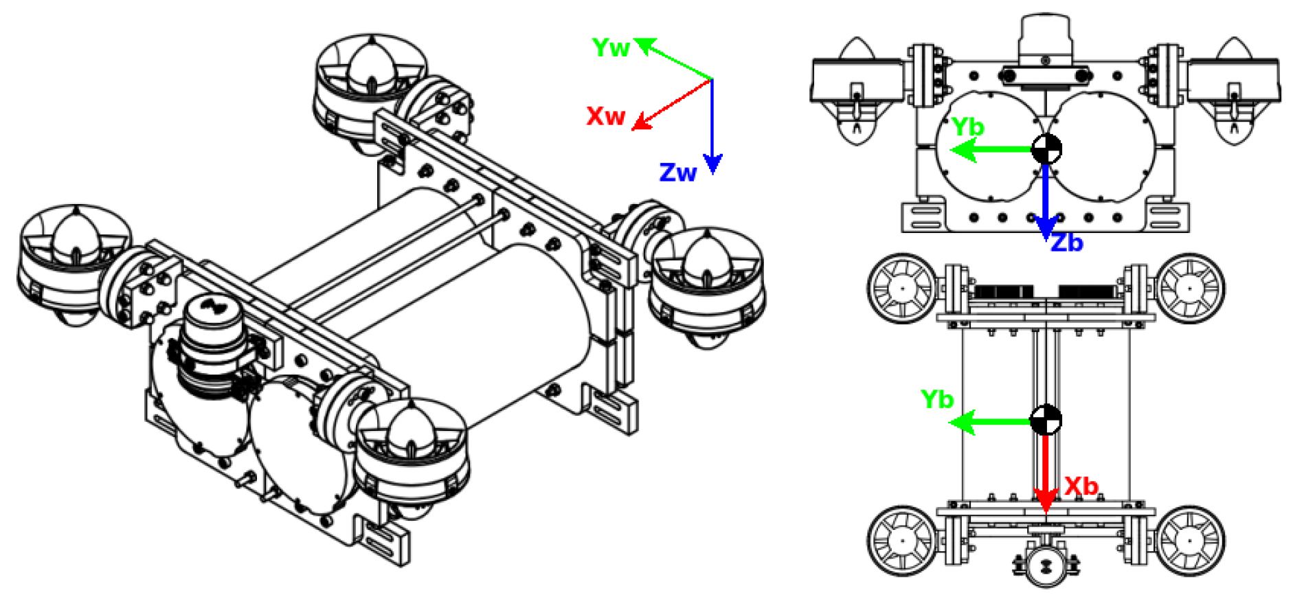
Figure 1.
Visualisation of the centre of mass (com) from two different points of view. Subindex ”w” means with respect to the world frame, while subindex ”b” means with respect to the body frame.
Figure 1.
Visualisation of the centre of mass (com) from two different points of view. Subindex ”w” means with respect to the world frame, while subindex ”b” means with respect to the body frame.
Figure 2.
The proposed methodology for obtaining the hydrodynamic coefficients from the experimental procedure. On the right side, the two experiments based on free decay tests are shown. On the left side, a description of the simulation procedure to obtain the values for the drag coefficient and linear and nonlinear term coefficients is shown.
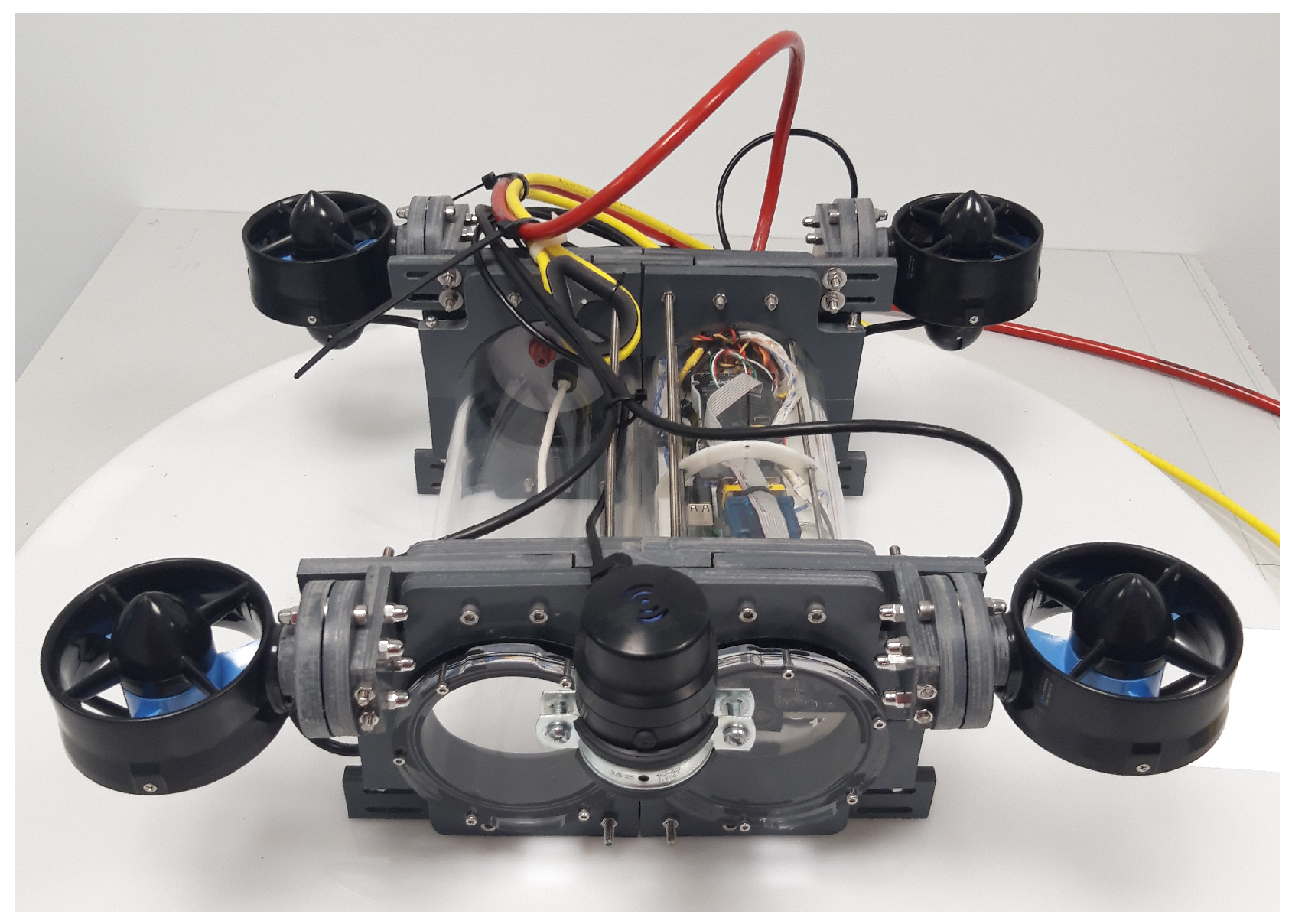
Figure 3.
The underwater drone robot. The right enclosure is used for the robot’s movement and navigation electronics, and the left enclosure is used for the waterproof payload (e.g., the electronics for a robotic arm).
Figure 3.
The underwater drone robot. The right enclosure is used for the robot’s movement and navigation electronics, and the left enclosure is used for the waterproof payload (e.g., the electronics for a robotic arm).
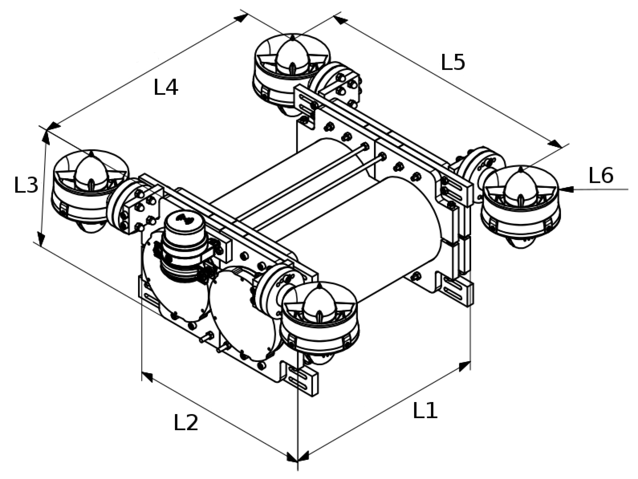
Figure 4.
In this schema, the lengths of the robots can be seen. These measurements take into account the dimensions of the experimental models. The values for the real robot are shown in
Table 1.
Figure 4.
In this schema, the lengths of the robots can be seen. These measurements take into account the dimensions of the experimental models. The values for the real robot are shown in
Table 1.
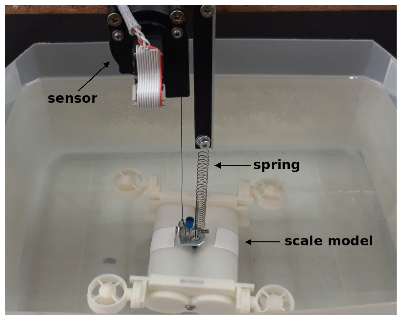
Figure 5.
The scheme used for the free decay test, where y is the length displacement of the model when it is oscillating and K is the spring constant. The sensor is a linear encoder, from which the information is sent to the Arduino, which records the data using the ROS framework. Afterward, the information is processed using the Matlab software.
Figure 6.
The values for the free decay test are obtained using the recovery force from a spring. The parameters required for obtaining the values used in this case are shown in
Table 2.
Figure 6.
The values for the free decay test are obtained using the recovery force from a spring. The parameters required for obtaining the values used in this case are shown in
Table 2.
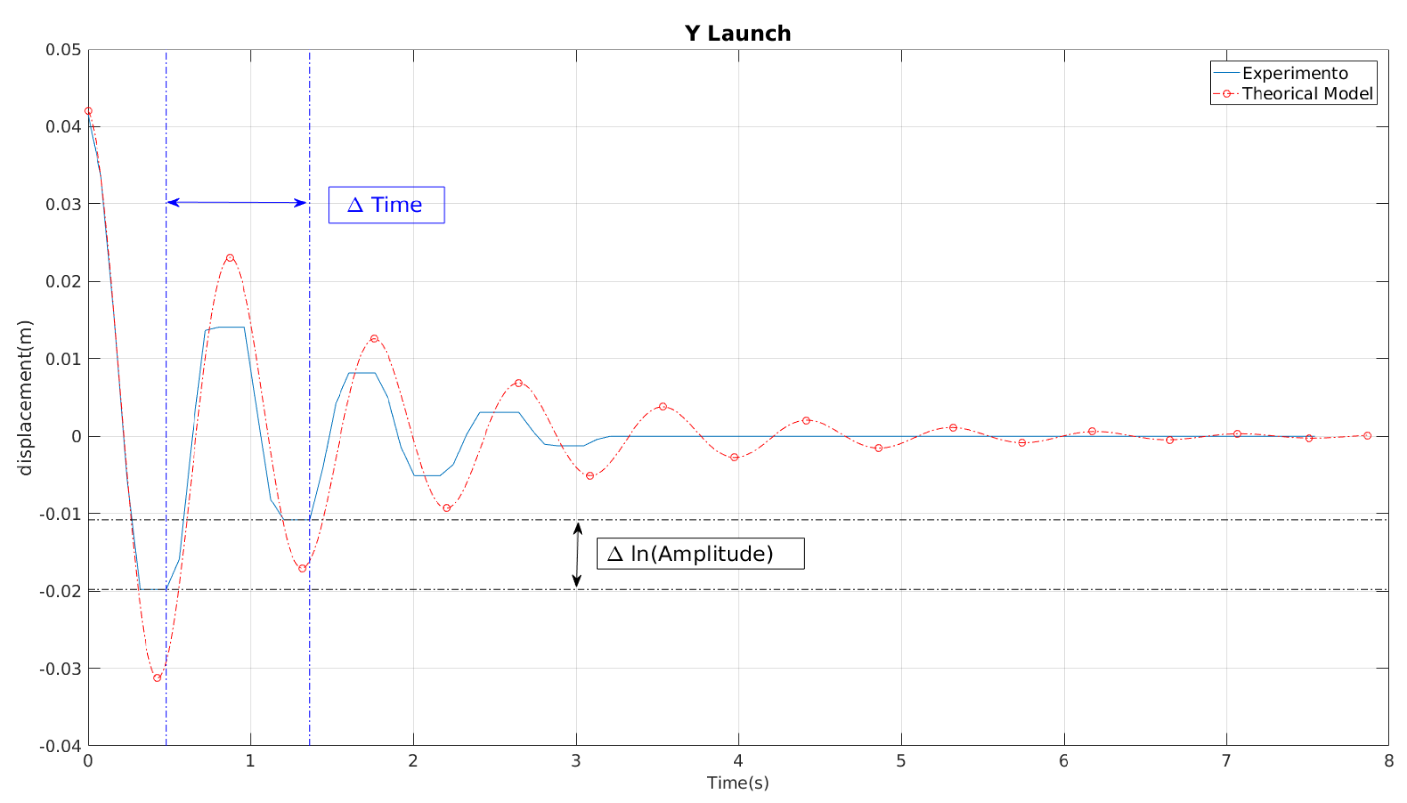
Figure 7.
The behaviour of a launch on the Y-axis for 4 cm of amplitude. The value of (time) is the distance between two consecutive peaks. The value of (ln(Amplitude)) is the logarithmic variation between the two values. The blue line is the result of the experiment and the red line is the response of the reconstructed model from those values.
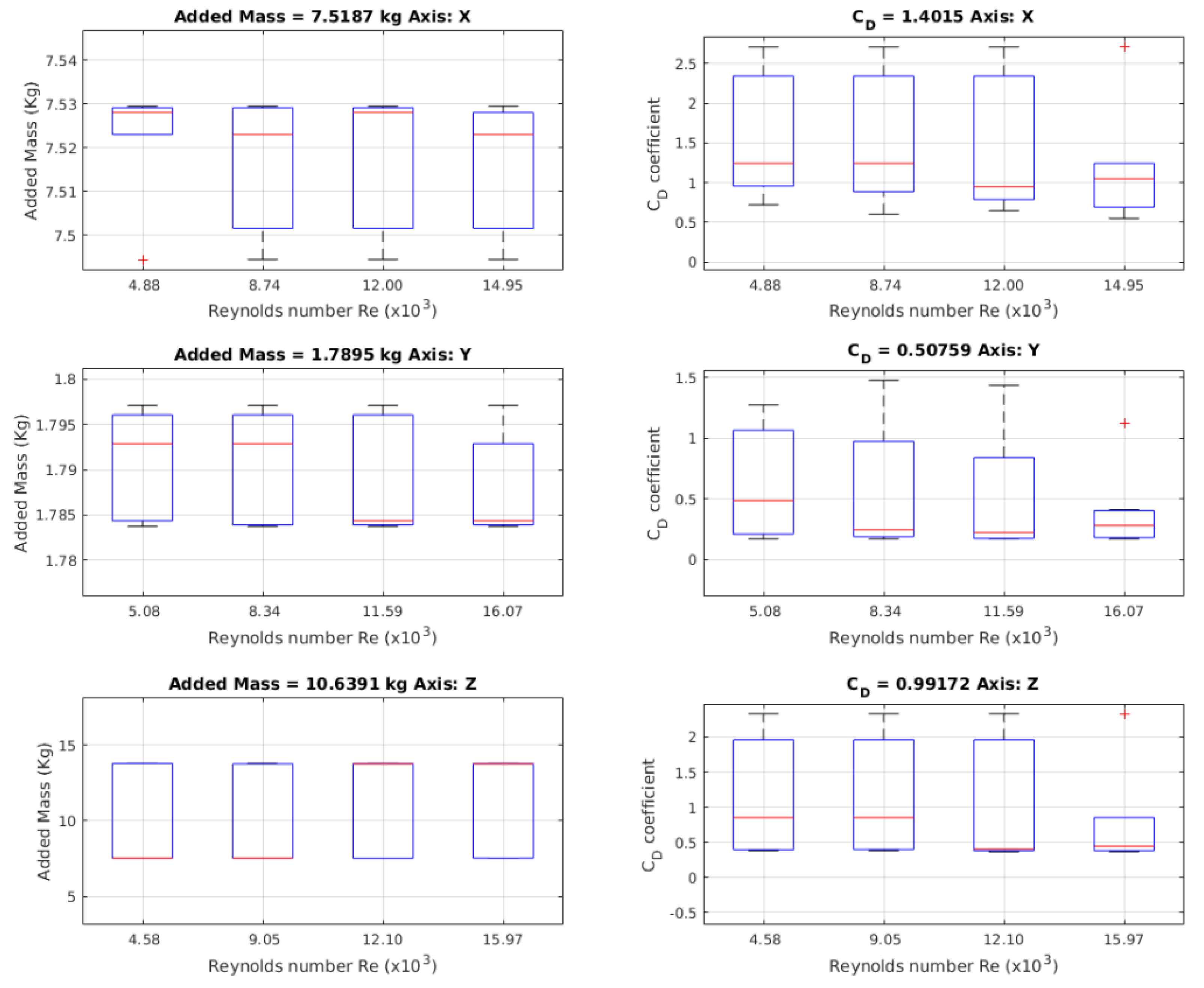
Figure 8.
Values for the added mass obtained using a free decay experiment by least squares as in the Chin method. On the left, the results for the values for added mass are shown. On the right, the values of drag coefficients are shown.
Figure 8.
Values for the added mass obtained using a free decay experiment by least squares as in the Chin method. On the left, the results for the values for added mass are shown. On the right, the values of drag coefficients are shown.
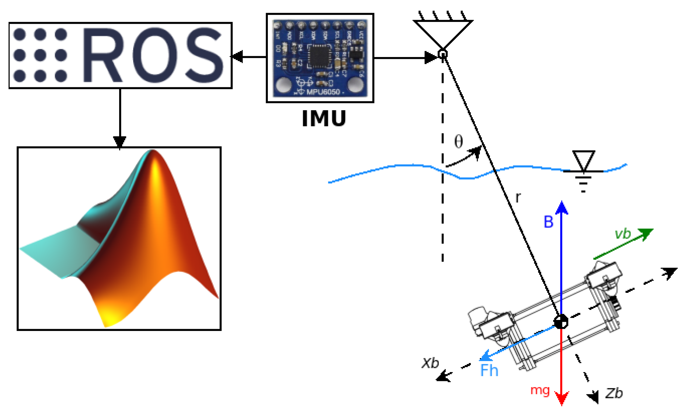
Figure 9.
On the right, the free body diagram used for modelling the body oscillating underwater is shown, where is the angle; r is the pendulum length; B is the buoyancy; m is the mass; g is the gravity acceleration (9.79 ); v is the body velocity; X and Z are the axes of the reference body system, respectively; and F is the hydrodynamical force. The angle is measured by an IMU, which sends the info to ROS, after which it is processed in Matlab.
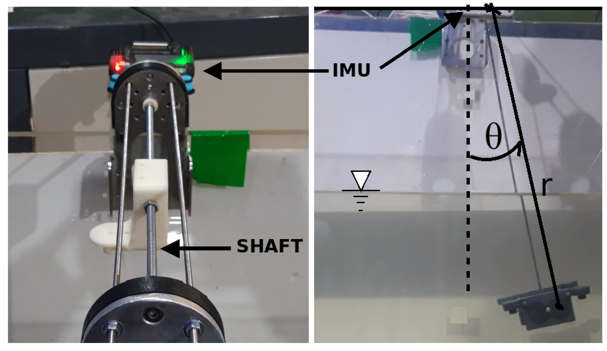
Figure 10.
Diagram of the free decay pendulum test, where is the angle with respect to the stability point and L is the length of the pendulum.
Figure 10.
Diagram of the free decay pendulum test, where is the angle with respect to the stability point and L is the length of the pendulum.
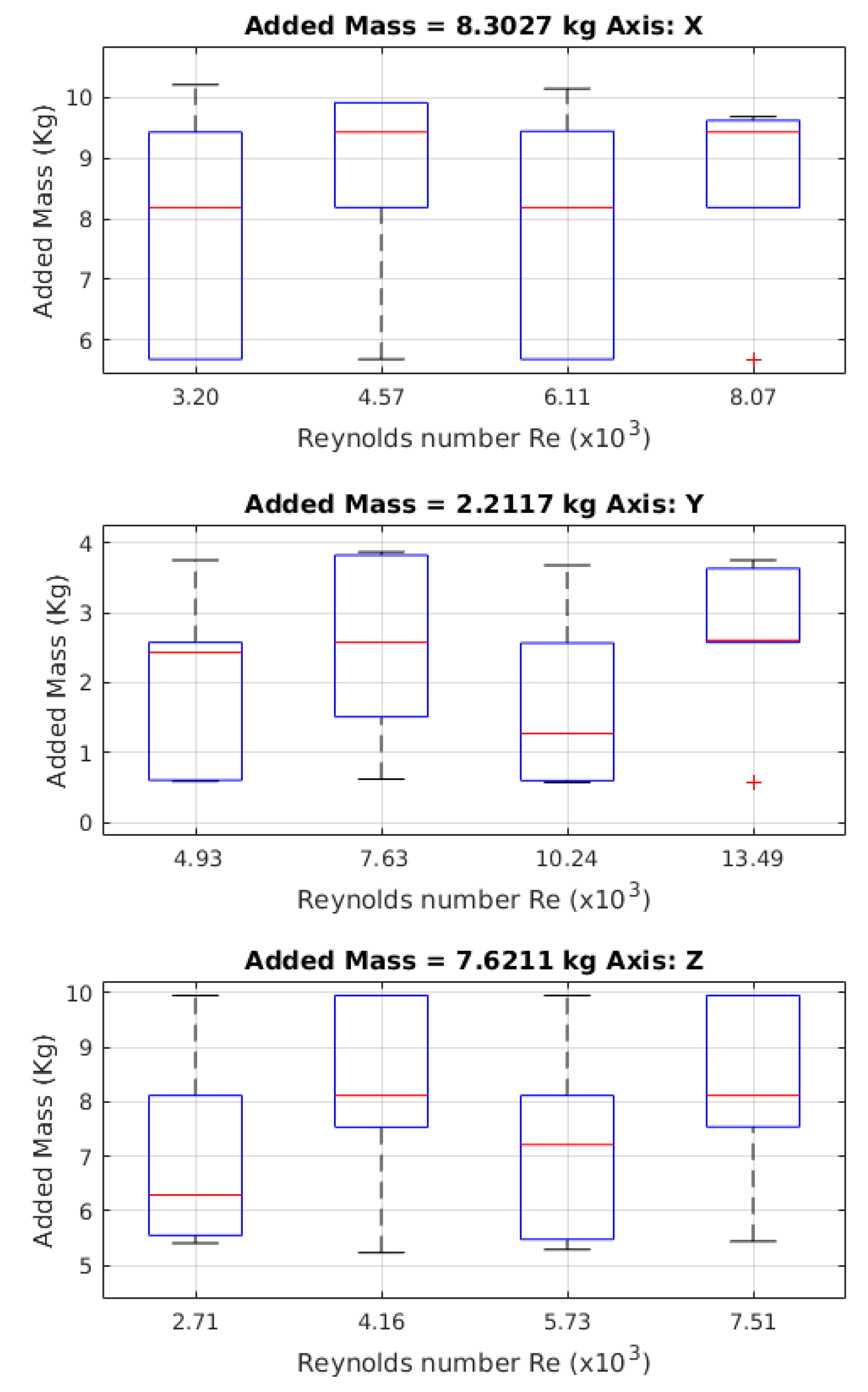
Figure 11.
Values obtained for the mass added using the free decay pendulum test. The values of the red crosses are outliers.
Figure 11.
Values obtained for the mass added using the free decay pendulum test. The values of the red crosses are outliers.
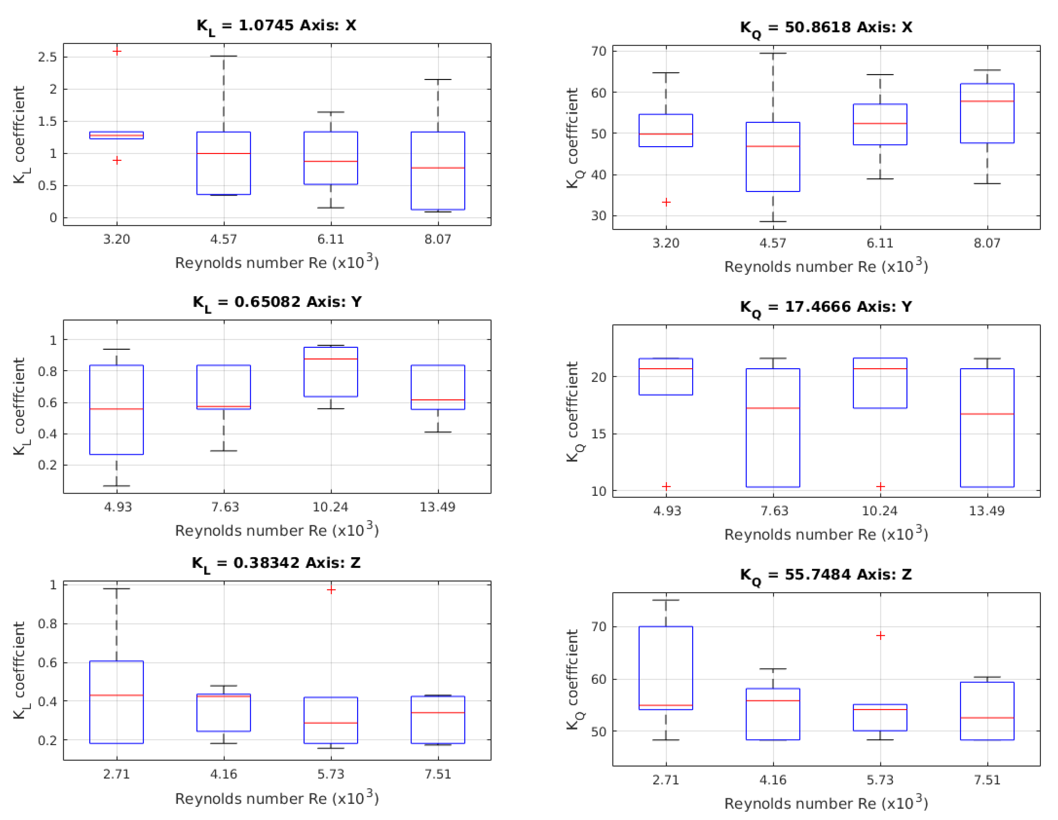
Figure 12.
Values of the linear coefficient obtained in the free decay pendulum test. This value is not present in the Morison equation, but is added to take into account other hydrodynamic phenomena.
Figure 12.
Values of the linear coefficient obtained in the free decay pendulum test. This value is not present in the Morison equation, but is added to take into account other hydrodynamic phenomena.
Figure 13.
Values for the added mass using the Morison equation for the free decay pendulum test. This is a novel implementation to obtain these values for this kind of test.
Figure 13.
Values for the added mass using the Morison equation for the free decay pendulum test. This is a novel implementation to obtain these values for this kind of test.
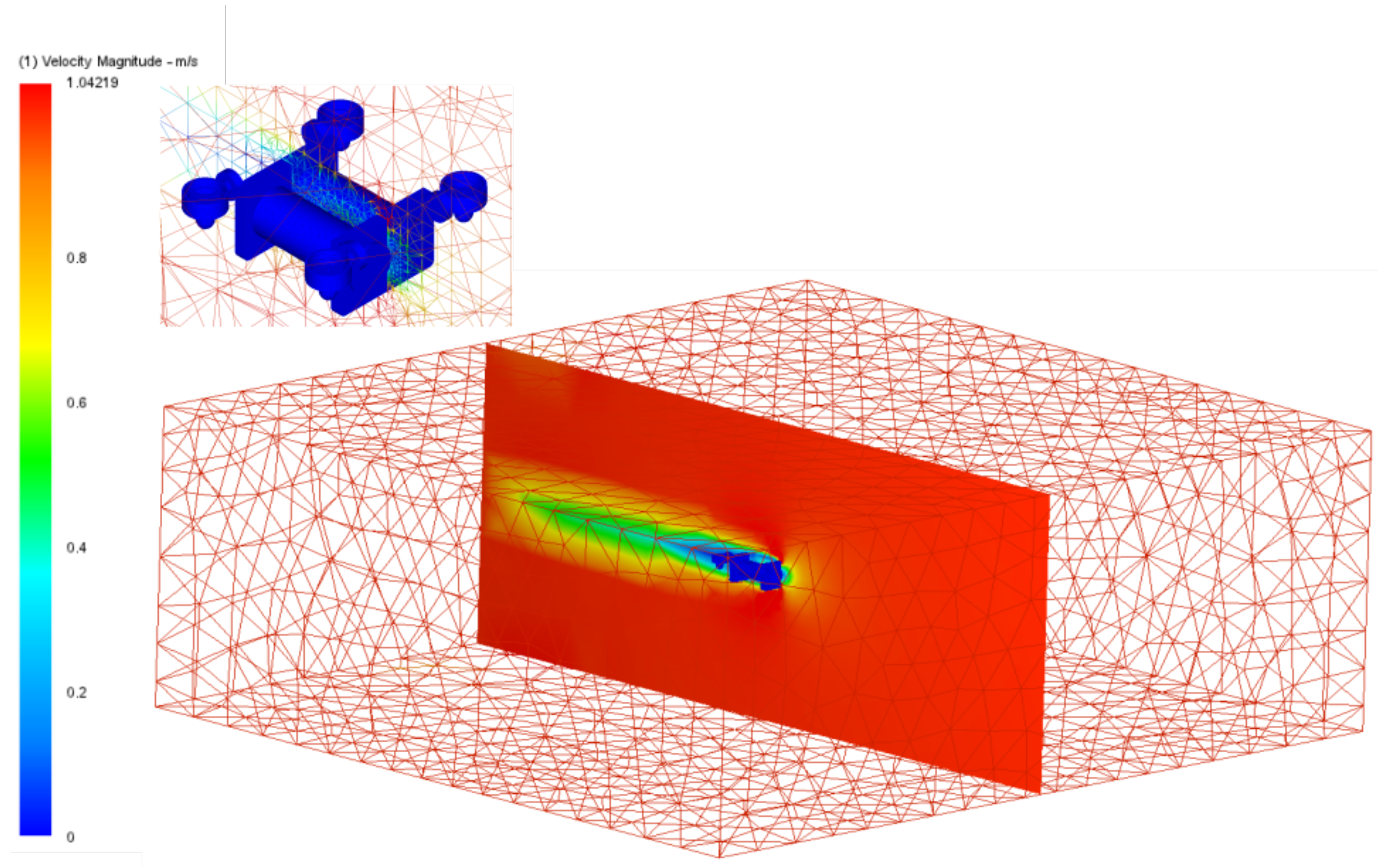
Figure 14.
The mesh used in the simulation of the Autodesk CFD software. The size corresponds to the volume used for the fluid, which is considered to have a distance of at least 10 times the length of the robot on that axis. At the top, the variation of the triangle size in the mesh near to the robot is shown. The robot is in blue.
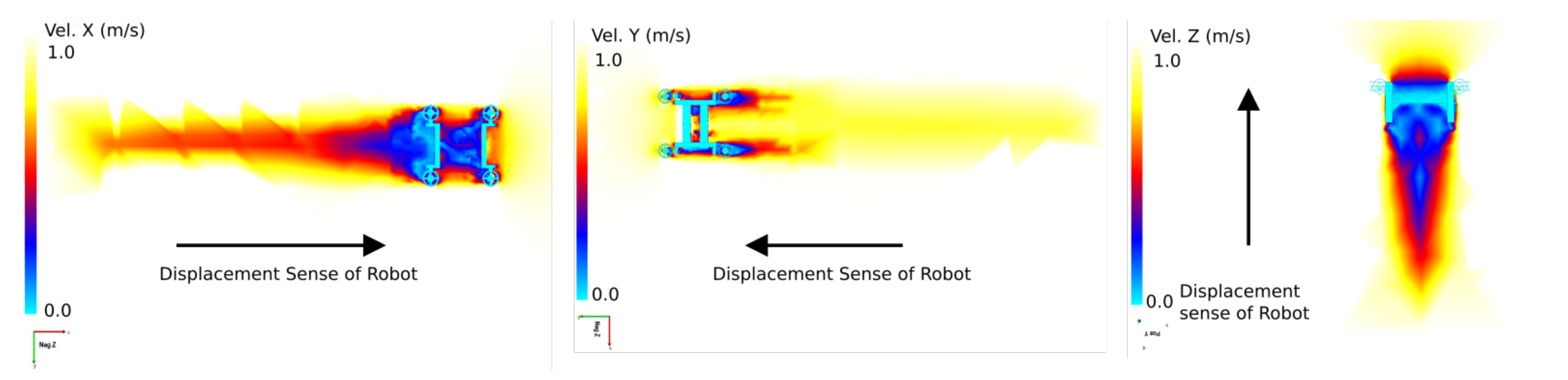
Figure 15.
Three different results for the CFD simulation. On the left, velocity is shown in the X-axis. In the middle it is shown in the Y-axis and on the right in the Z-axis. These results were obtained at 1 . The dark blue zones are values close to 0 .
Figure 15.
Three different results for the CFD simulation. On the left, velocity is shown in the X-axis. In the middle it is shown in the Y-axis and on the right in the Z-axis. These results were obtained at 1 . The dark blue zones are values close to 0 .
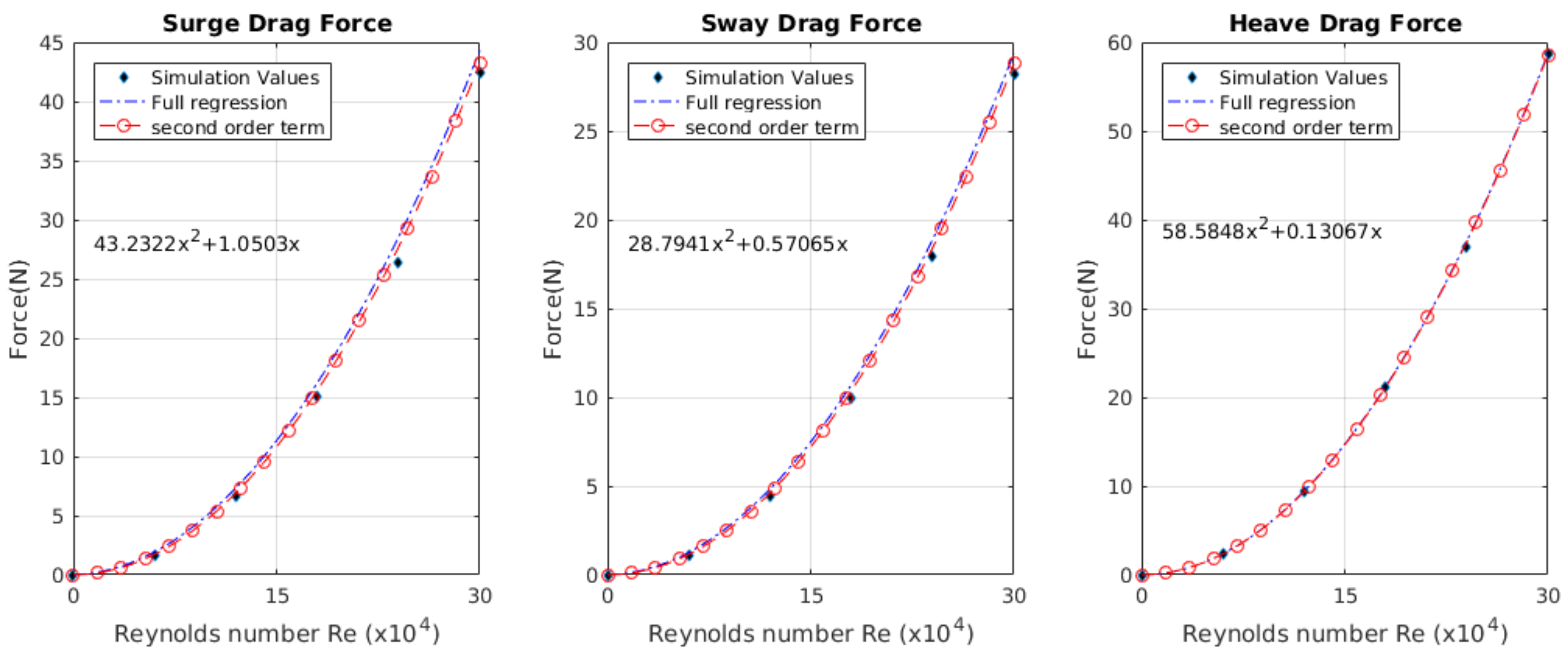
Figure 16.
The values of the regressions obtained for the X, Y and Z axes, in terms of their surge, sway, and heave speeds, respectively. The black diamonds are the values obtained using the CFD simulation, the regression with all the terms is the dotted blue line and the red line shows the model using just the quadratic coefficient.
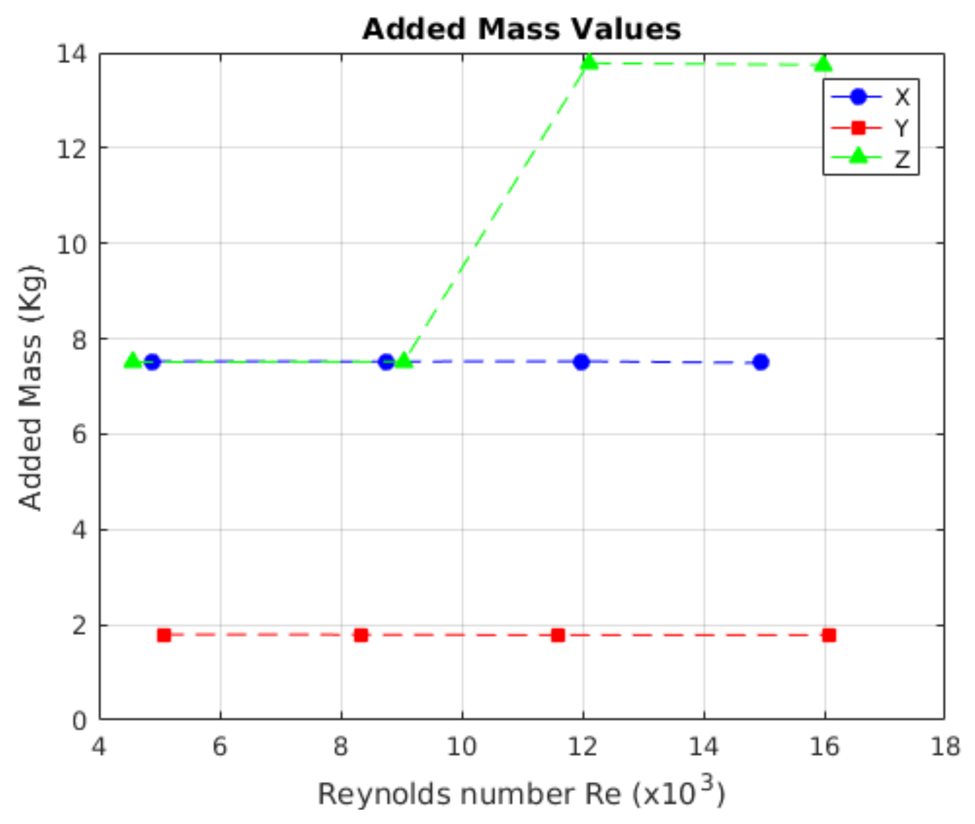
Figure 17.
Behaviour of the added mass. The values for each axis are similar at all speeds.
Figure 17.
Behaviour of the added mass. The values for each axis are similar at all speeds.
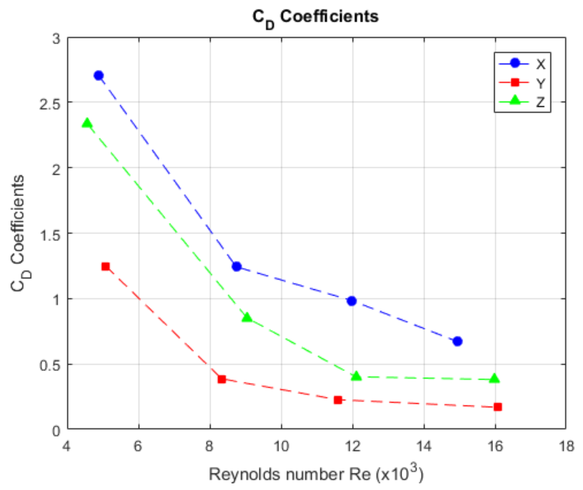
Figure 18.
The behaviour of the value of the drag coefficient with respect to the speed in Reynolds number.
Figure 18.
The behaviour of the value of the drag coefficient with respect to the speed in Reynolds number.
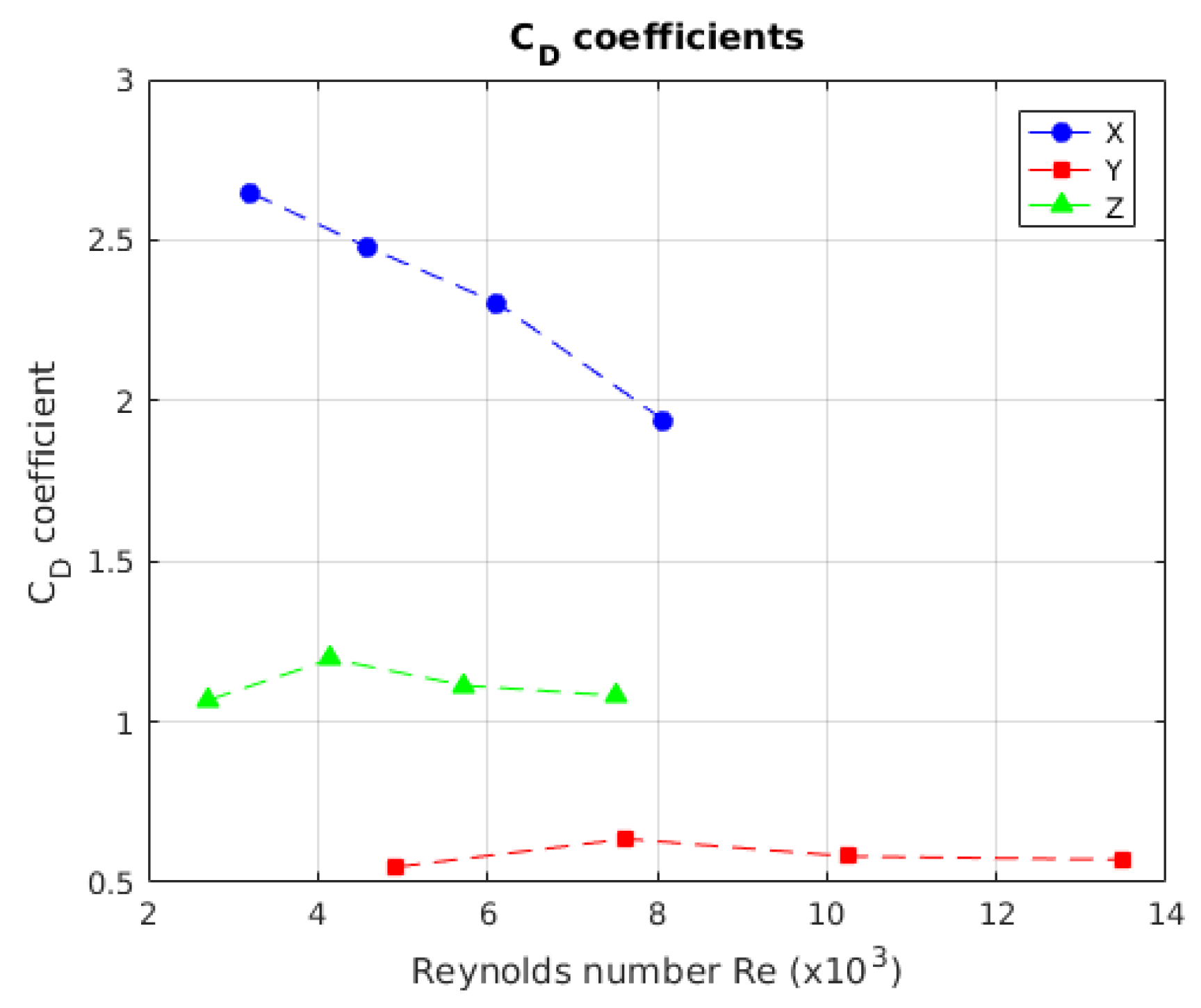
Figure 19.
Behaviour of the drag coefficient with respect to speed. It is not possible to determine a characteristic behaviour for each axis.
Figure 19.
Behaviour of the drag coefficient with respect to speed. It is not possible to determine a characteristic behaviour for each axis.
Table 1.
Physical characteristics of the real robot
Table 1.
Physical characteristics of the real robot
| Dimension | Value |
|---|
| Weight (kg) | 9.36 |
| Volume (mm) | 528,797 |
| L1 (m) | 0.298 |
| L2 (m) | 0.269 |
| L3 (m) | 0.169 |
| L4 (m) | 0.348 |
| L5 (m) | 0.395 |
| L6 (m) | 0.045 |
Table 2.
Parameters of the model for the free decay test.
Table 2.
Parameters of the model for the free decay test.
| Parameter | Value |
|---|
| Weight (kg) | 0.97 |
| Volume (mm) | 344,868 |
| Material | Acrylonitrile butadiene styrene (ABS) and lead |
| Scale | 30% |
Table 3.
Parameters of the model for the free decay pendulum test.
Table 3.
Parameters of the model for the free decay pendulum test.
| Parameter | Value |
|---|
| Weight (kg) | 0.146 |
| Volume (mm) | 107,597 |
| Material | PVC |
| Scale | 22% |
Table 4.
Summary of parameters for the Computational Fluid Dynamic (CFD) simulation configuration.
Table 4.
Summary of parameters for the Computational Fluid Dynamic (CFD) simulation configuration.
| Mesh Configuration | Solver Setting |
|---|
| Resolution factor | 1 | Solution mode | Transient |
| Edge growth rate | 1.1 | Advection scheme | Monotone streamline upwind |
| Layer factor | 0.45 | Turbulence model | k-epsilon |
| Layer gradation | 1.05 | Time step size | 0.1 s |
| Number of nodes | 46,879 | Iterations | 500 |
| Number of elements | 204,258 | Time Stop | 50 s |
Table 5.
Values Obtained through the CFD Simulation.
Table 5.
Values Obtained through the CFD Simulation.
| Axis | X | Y | Z |
|---|
| K Coefficient | 1.0503 | 0.5706 | 0.1306 |
| K Coefficient | 43.2322 | 28.7941 | 58.5848 |
| R | 0.9960 | 0.9963 | 0.9967 |
| K Coefficient | 42.0253 | 28.1384 | 58.4346 |
| Coefficient | 1.7021 | 0.6226 | 1.2929 |
| R | 0.9961 | 0.9964 | 0.9967 |
Table 6.
Stochastic values for added mass in the free decay test.
Table 6.
Stochastic values for added mass in the free decay test.
| | | X | Y | Z |
|---|
| L | L | p-value | p-value | p-value |
| z-value | z-value | z-value |
| 1 | 2 | 0.1983 | 0.1202 | 0.0393 |
| −1.286 | −1.553 | 2.0603 |
| 1 | 3 | 1.0000 | 0.4382 | 0.0047 |
| 0 | −0.775 | 2.8235 |
| 1 | 4 | 0.6076 | 0.1210 | 1.0000 |
| 0.5133 | −1.550 | 0 |
| 2 | 3 | 0.0020 | 0.2470 | 1.0000 |
| 3.0836 | −1.157 | 0 |
| 2 | 4 | 0.6995 | 0.0717 | 0.5986 |
| −0.385 | −1.8 | −0.5263 |
| 3 | 4 | 0.2485 | 0.04 | 0.0127 |
| −1.153 | −2.053 | 0 |
Table 7.
Values obtained in the free decay test.
Table 7.
Values obtained in the free decay test.
| Axis | X | Y | Z |
|---|
| Damping Coefficient, | 0.1971 | 0.109 | 0.1418 |
| Drag Coefficient, | 1.4015 | 0.5075 | 0.9917 |
| Natural Frequency, () | 7.1142 | 7.8268 | 6.8188 |
| Added Mass Coefficient (Cm) | 0.8172 | 0.1945 | 1.1564 |
Table 8.
Stochastic values for K in the free decay pendulum test.
Table 8.
Stochastic values for K in the free decay pendulum test.
| | | X | Y | Z |
|---|
| L | L | p-value | p-value | p-value |
| z-value | z-value | z-value |
| 1 | 2 | 0.9362 | 0.8102 | 0.2980 |
| −0.080 | −0.240 | −1.040 |
| 1 | 3 | 0.3785 | 0.8102 | 0.2980 |
| −0.880 | −0.240 | −1.040 |
| 1 | 4 | 0.0656 | 0.8102 | 0.2280 |
| −1.841 | −0.240 | −1.201 |
| 2 | 3 | 0.3785 | 0.8102 | 0.8102 |
| −0.880 | −0.240 | −0.240 |
| 2 | 4 | 0.1735 | 0.8102 | 0.5752 |
| −1.361 | −0.240 | −0.560 |
| 3 | 4 | 0.9362 | 0.8102 | 1.0000 |
| −0.080 | −0.240 | 0.0 |
Table 9.
Stochastic values for K in the free decay pendulum test.
Table 9.
Stochastic values for K in the free decay pendulum test.
| | | X | Y | Z |
|---|
| L | L | p-value | p-value | p-value |
| z-value | z-value | z-value |
| 1 | 2 | 0.1735 | 0.4712 | 0.2298 |
| −1.361 | 0.7205 | −1.201 |
| 1 | 3 | 0.3785 | 0.0453 | 0.5752 |
| 0.8807 | 2.0016 | 0.5604 |
| 1 | 4 | 0.6889 | 0.0082 | 0.0131 1 |
| 0.4003 | 2.6421 | 2.482 |
| 2 | 3 | 0.3785 | 0.0927 | 0.0927 |
| 0.8807 | 1.6813 | 1.6813 |
| 2 | 4 | 0.2980 | 0.0131 | 0.0051 |
| 1.0408 | 2.482 | 2.8022 |
| 3 | 4 | 0.8102 | 0.4712 | 0.1735 |
| 0.2401 | 0.7205 | 1.3611 |
Table 10.
Values Obtained through the free decay pendulum test.
Table 10.
Values Obtained through the free decay pendulum test.
| Axis | X | Y | Z |
|---|
| K Coefficient | 1.0745 | 0.6508 | 0.3834 |
| K Coefficient | 50.8618 | 17.4666 | 55.7484 |
| Coefficient | 2.3432 | 0.5838 | 1.1145 |
| Added Mass Coefficient (Cm) | 0.9024 | 0.2404 | 0.8283 |


