Performance Improvement of Time-Differenced Carrier Phase Measurement-Based Integrated GPS/INS Considering Noise Correlation

Abstract
:1. Introduction
2. Theory
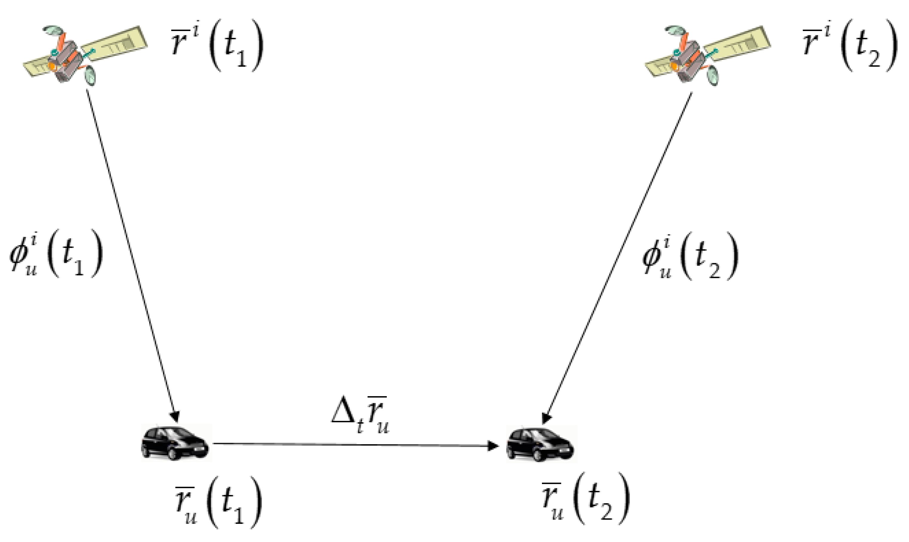
2.1. Time-Differenced Carrier Phase (TDCP) Measurements
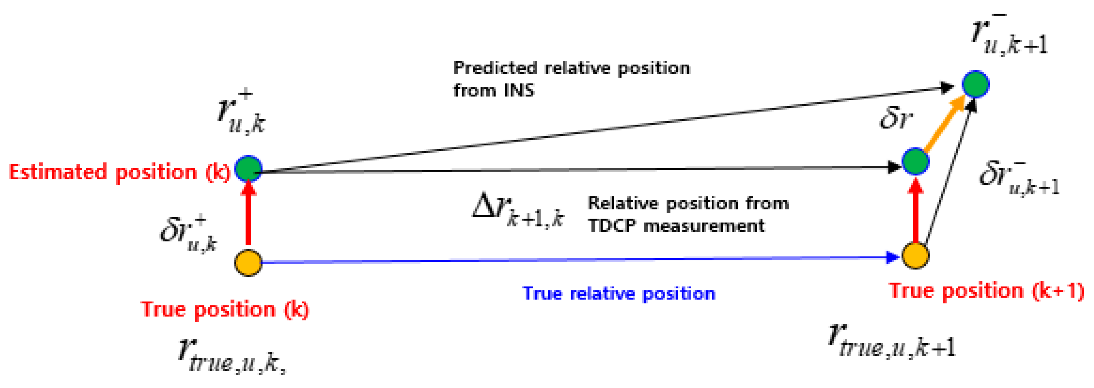
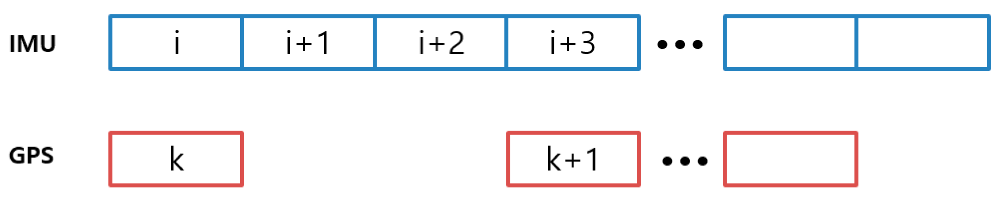
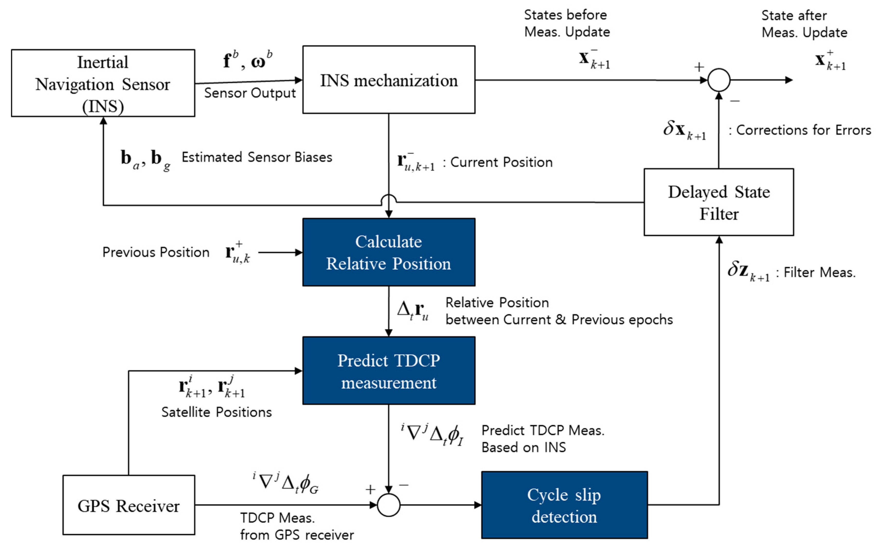
2.2. TDCP-Based Global Positioning System/Inertial Navigation System (GPS/INS).
3. Simulation and Experimental Results
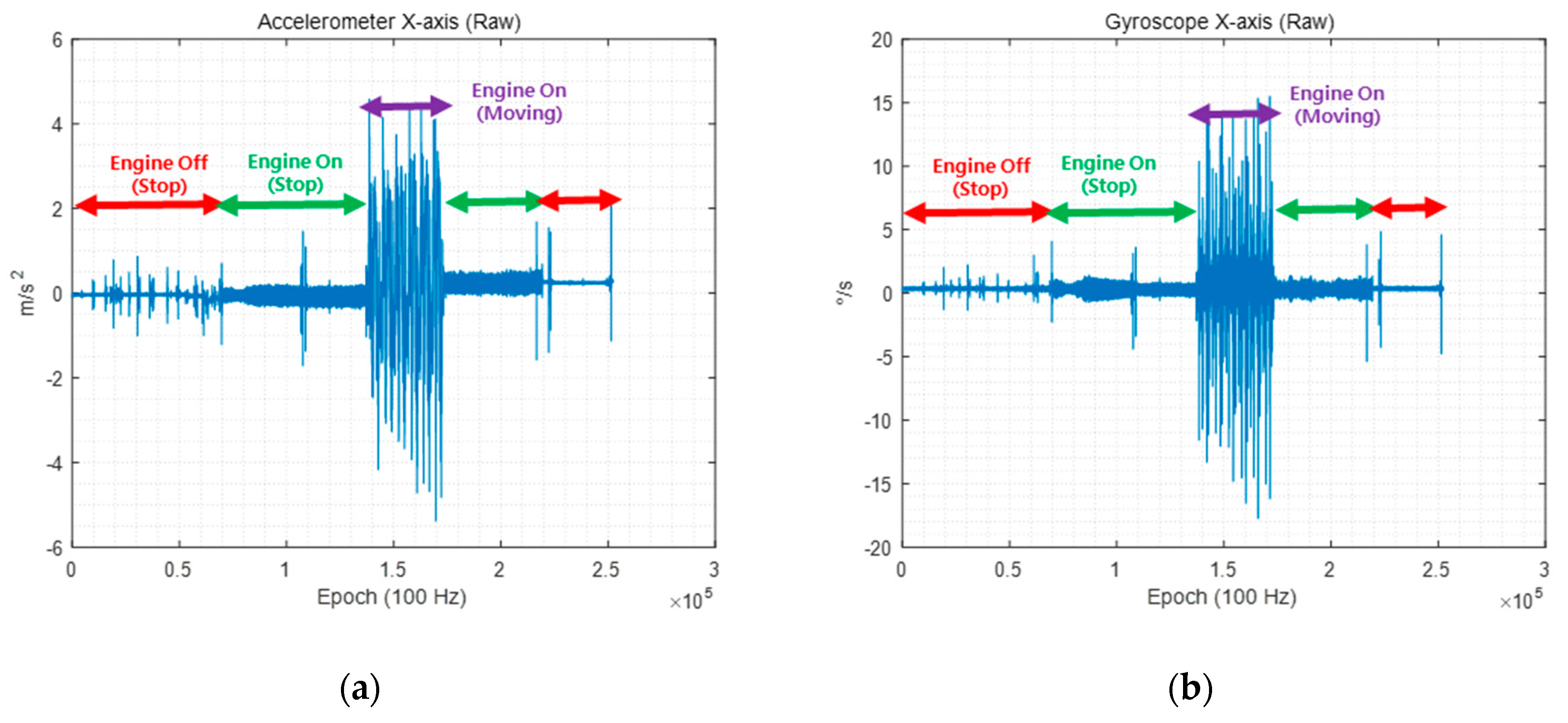
3.1. Preliminary Test
3.2. Simulation
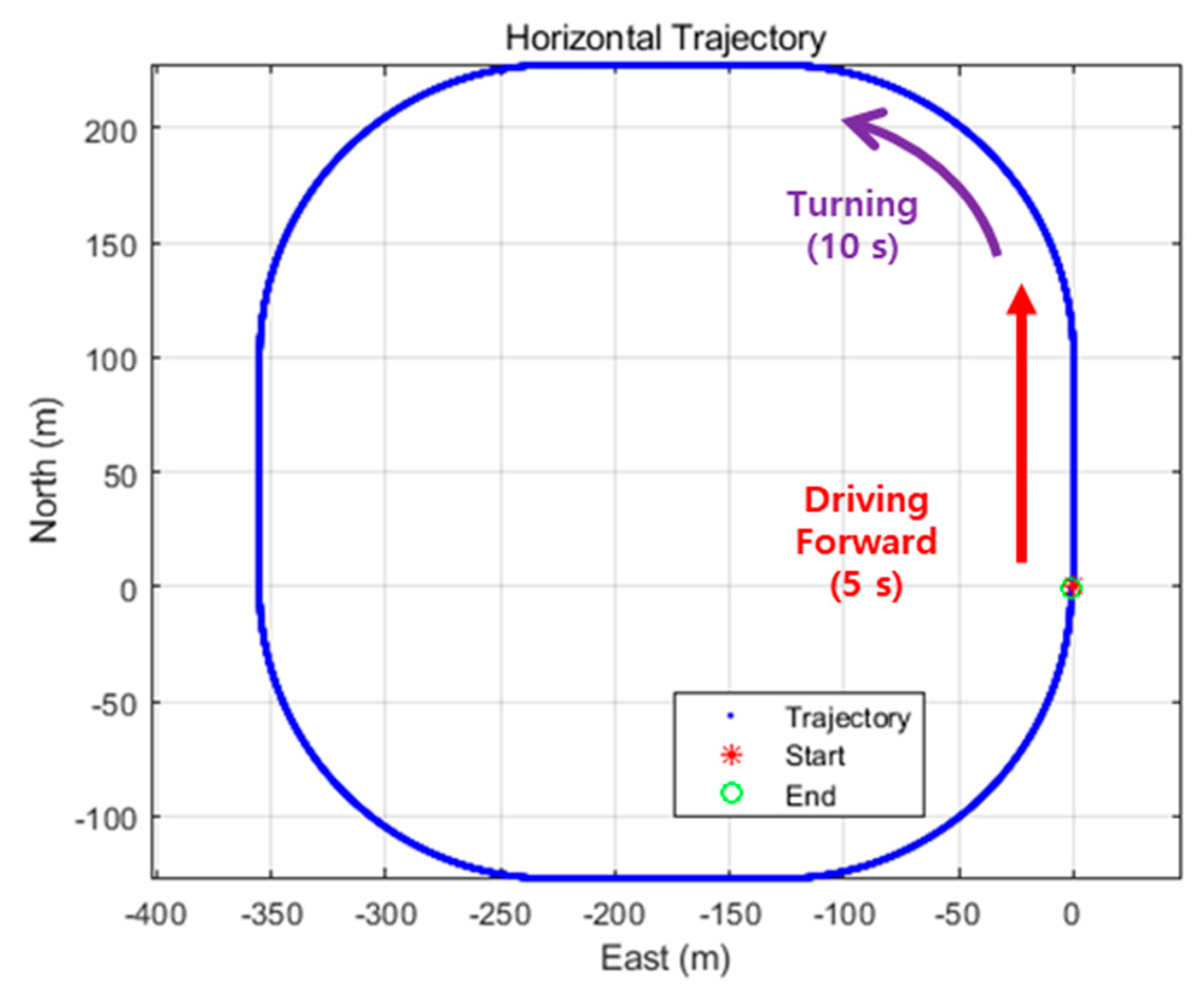
3.2.1. Simulation Environment
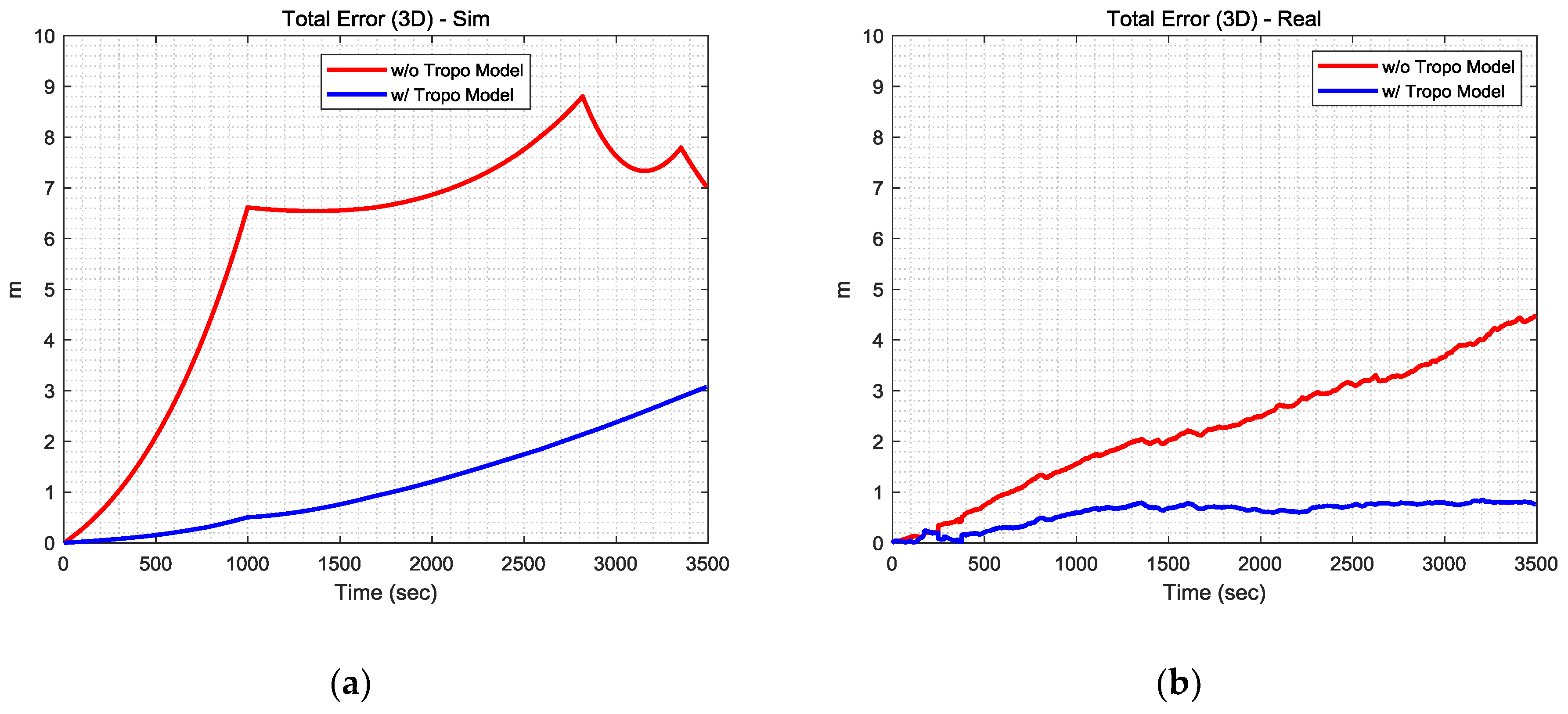
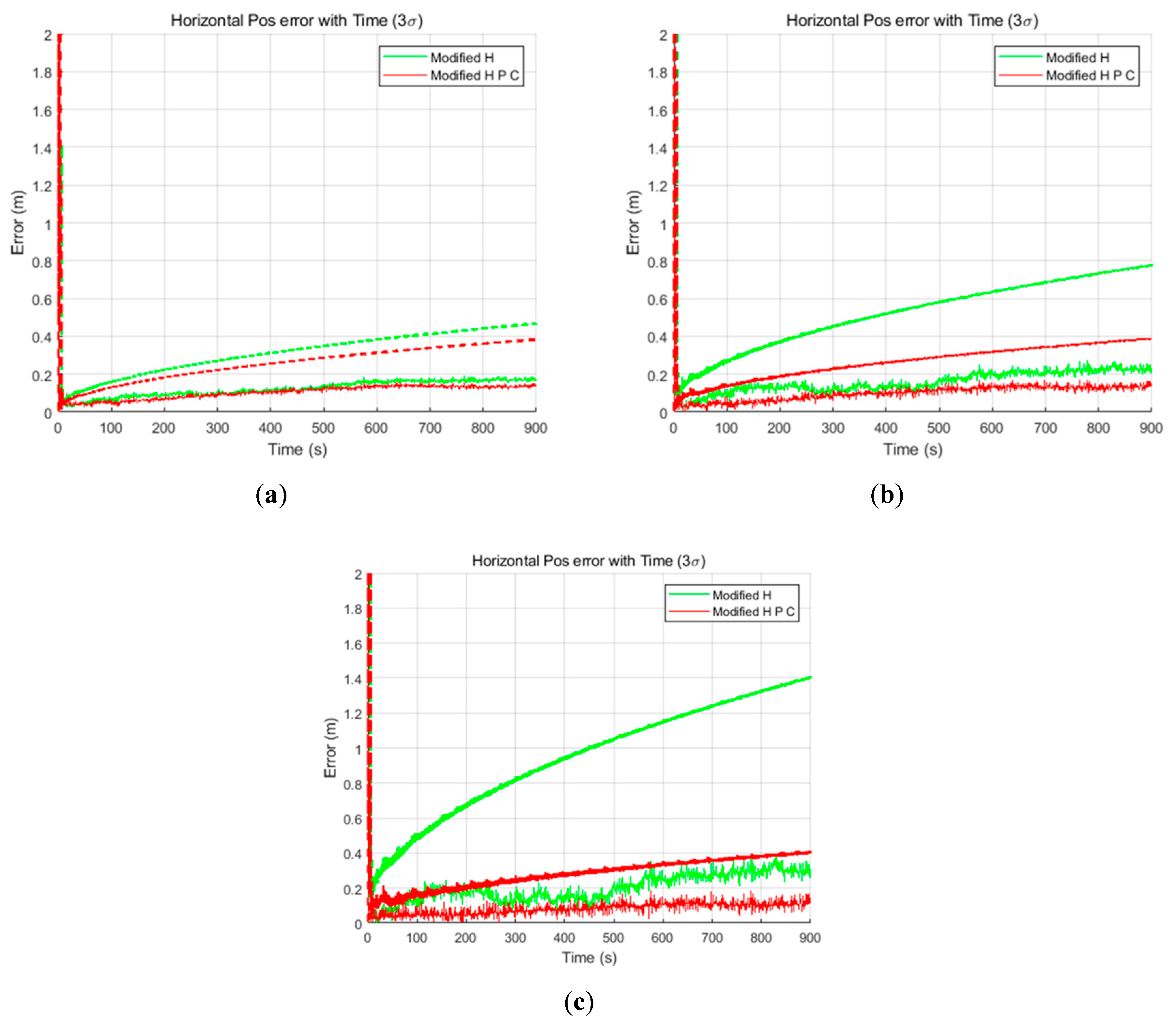
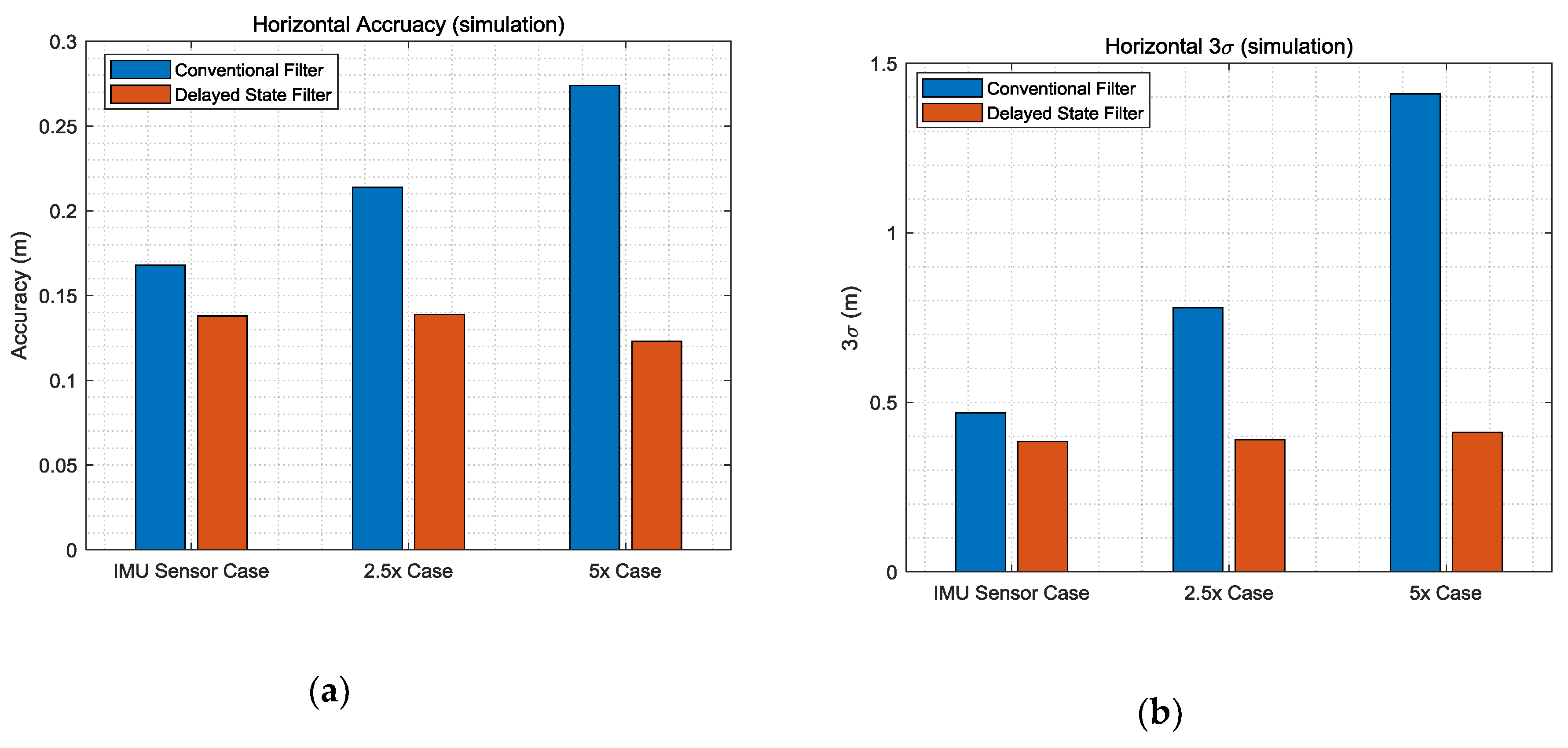
3.2.2. Simulation Results
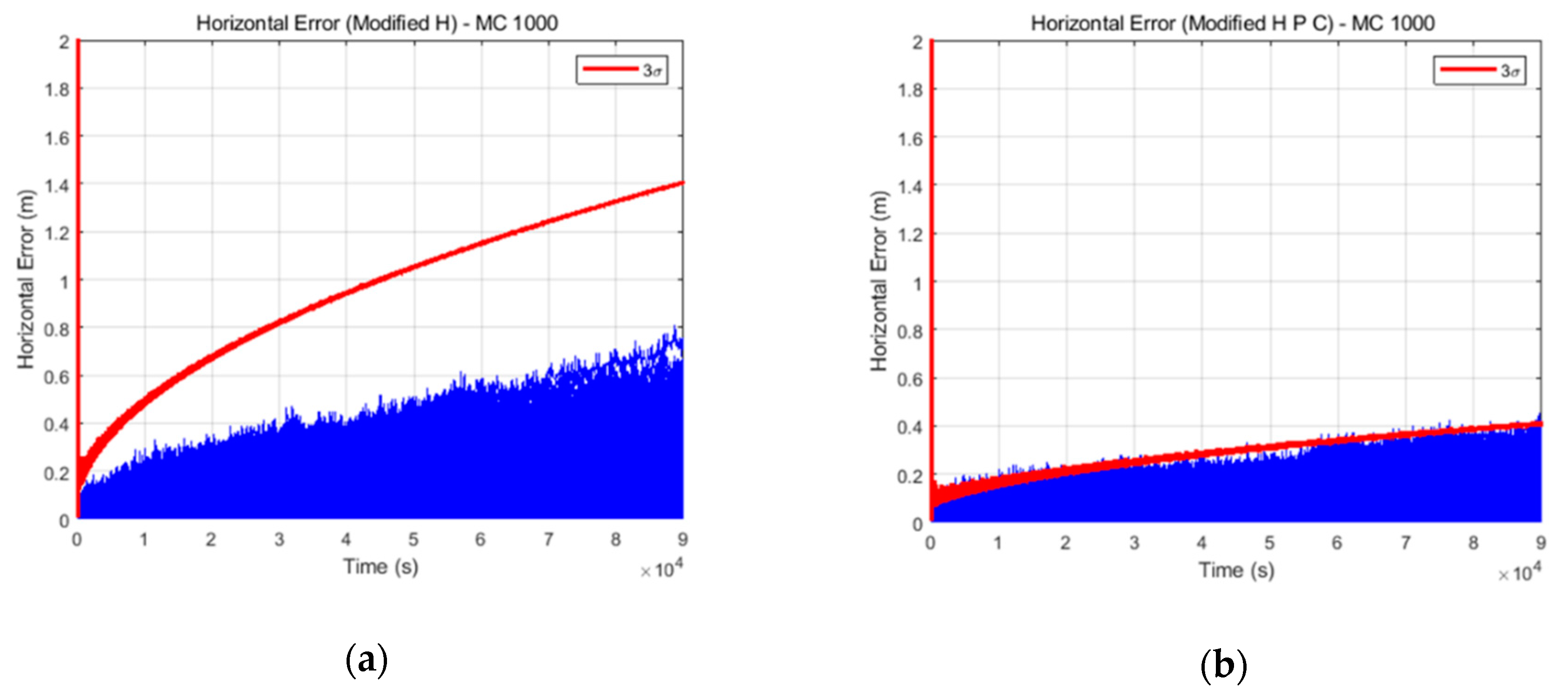
3.2.3. Monte Carlo Simulation Results
3.3. Experiment
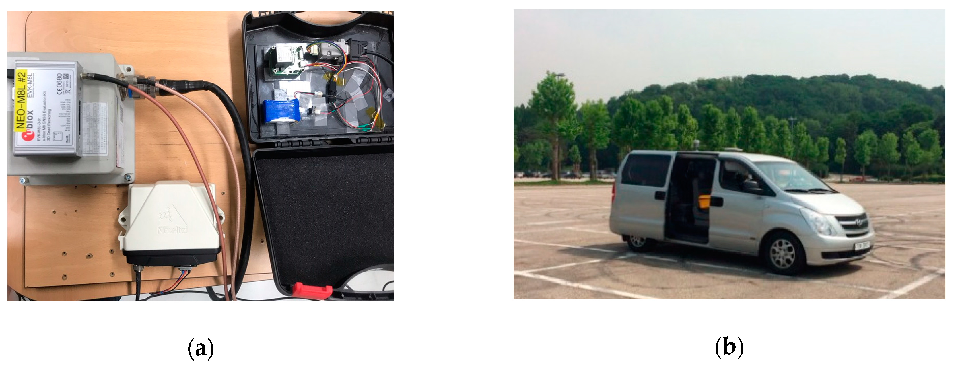
3.3.1. Experimental Environment
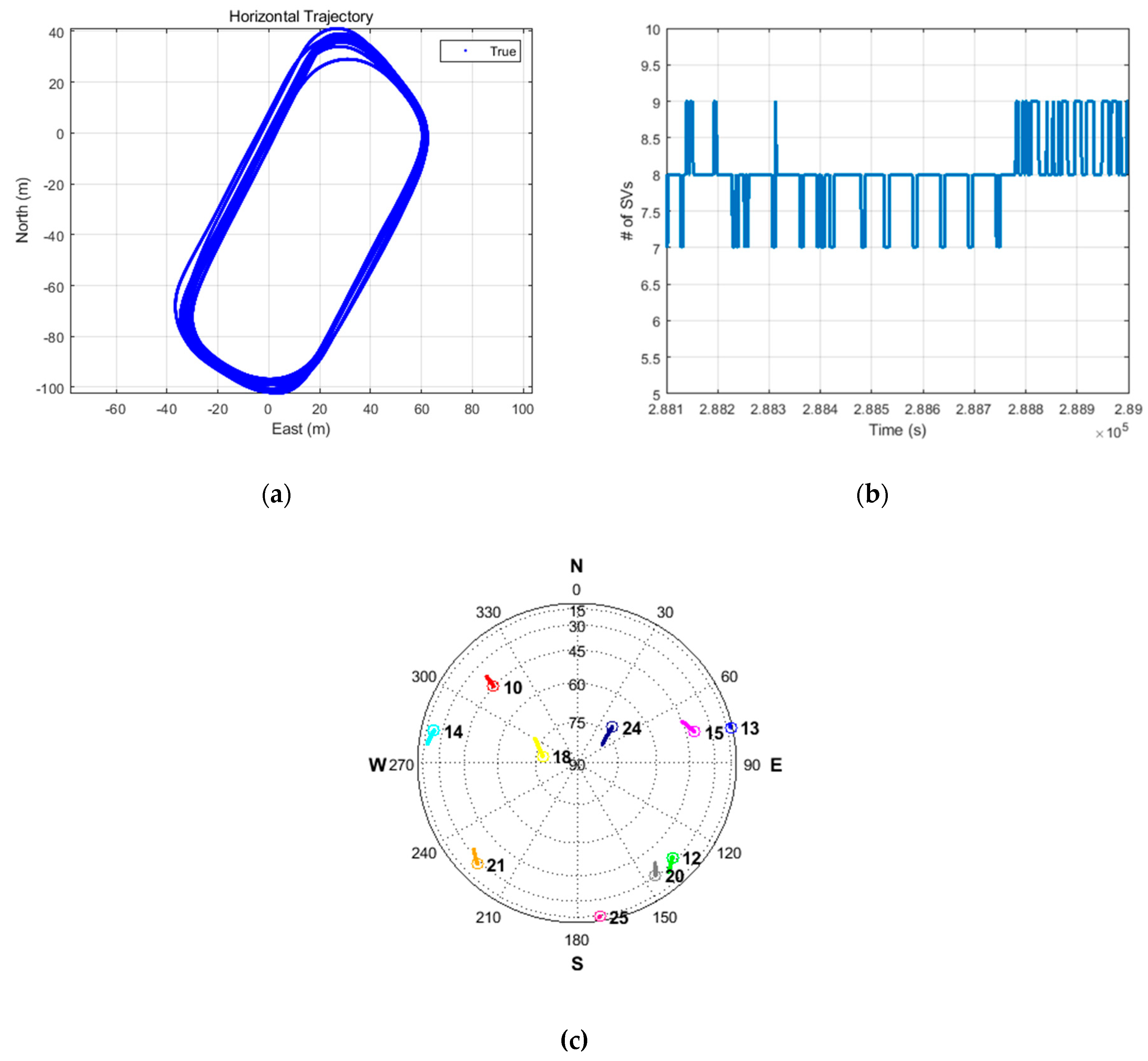
3.3.2. Experimental Results
4. Conclusions
Author Contributions
Funding
Conflicts of Interest
References
- Hieu, L.N.; Nguyen, V.H. Loosely Coupled GPS/INS Integration with Kalman Filtering for Land Vehicle Applications. In Proceedings of the 2012 International Conference on Control, Automation and Information Sciences (ICCAIS), Ho Chi Minh City, Vietnam, 26–29 November 2012. [Google Scholar]
- Yoon, D.; Kee, C.; Seo, J.; Park, B. Position accuracy improvement by implementing the DGNSS-CP algorithm in smartphones. Sensors 2016, 16, 910. [Google Scholar] [CrossRef] [PubMed]
- Ding, W.; Wang, J.; Rizos, C.; Kinlyside, D. Improving adaptive kalman estimation in GPS/INS integration. J. Navig. 2007, 60, 517–529. [Google Scholar] [CrossRef]
- Falco, G.; Pini, M.; Marucco, G. Loose and tight GNSS/INS integrations: Comparison of performance assessed in real urban scenarios. Sensors 2017, 17, 255. [Google Scholar] [CrossRef] [PubMed]
- Li, Z.; Wang, D.; Dong, Y.; Wu, J. An enhanced tightly-coupled integrated navigation approach using phase-derived position increment (PDPI) measurement. Optik (Stuttg) 2018, 156, 135–147. [Google Scholar] [CrossRef]
- Teunissen, P.J.G.; De Jonge, P.J.; Tiberius, C.C.J.M. Performance of the LAMBDA Method for Fast GPS Ambiguity Resolution. Navigation 1997, 44, 373–383. [Google Scholar] [CrossRef]
- Takasu, T.; Yasuda, A. Kalman-filter-based integer ambiguity resolution strategy for long-baseline RTK with ionosphere and troposphere estimation. Ion Ntm 2010, 2010, 161–171. [Google Scholar]
- Cai, C.; Gao, Y. Precise Point Positioning Using Combined GPS and GLONASS Observations. J. Glob. Position. Syst. 2007, 6, 13–22. [Google Scholar] [CrossRef] [Green Version]
- Ding, W.; Wang, J. Precise velocity estimation with a stand-alone GPS receiver. J. Navig. 2011, 64, 311–325. [Google Scholar] [CrossRef]
- Soon, B.K.H.; Scheding, S.; Lee, H.K.; Lee, H.K.; Durrant-Whyte, H. An approach to aid INS using time-differenced GPS carrier phase (TDCP) measurements. GPS Solut. 2008, 12, 261–271. [Google Scholar] [CrossRef]
- Freda, P.; Angrisano, A.; Gaglione, S.; Troisi, S. Time-differenced carrier phases technique for precise GNSS velocity estimation. GPS Solut. 2015, 19, 335–341. [Google Scholar] [CrossRef]
- Wendel, J.; Trommer, G.F. Tightly coupled GPS/INS integration for missile applications. Aerosp. Sci. Technol. 2004, 8, 627–634. [Google Scholar] [CrossRef]
- Wendel, J.; Meister, O.; Mönikes, R.; Trommer, G.F. Time-differenced carrier phase measurements for tightly coupled GPS/INS integration. In Proceedings of the 2006 IEEE/ION Position, Location, And Navigation Symposium, San Diego, CA, USA, 25–27 April 2006. [Google Scholar]
- Han, S.; Wang, J. Integrated GPS/INS navigation system with dual-rate Kalman Filter. GPS Solut. 2012, 16, 389–404. [Google Scholar] [CrossRef]
- Zhao, Y. Applying Time-Differenced Carrier Phase in Nondifferential GPS/IMU Tightly Coupled Navigation Systems to Improve the Positioning Performance. IEEE Trans. Veh. Technol. 2017, 66, 992–1003. [Google Scholar] [CrossRef]
- Travis, W.E. Path Duplication Using GPS Carrier Based Relative Position for Automated Ground Vehicle Convoys; Auburn University: Auburn, AL, USA, 2010. [Google Scholar]
- RTCA SC-159. Minimum Operational Performance Standards for Global Positioning System/Wide Area Augmentation System Airborne Equipment; RTCA: Washington, DC, USA, 2006. [Google Scholar]
- Park, B. A Study on Reducing Temporal and Spatial Decorrelation Effect in GNSS Augmentation System: Consideration of the Correction Message Standardization; Seoul National University: Seoul, Korea, 2008. [Google Scholar]
- Crustal Dynamics Data Information System. Available online: https://cddis.nasa.gov/Data_and_Derived_Products/GNSS/atmospheric_products.html (accessed on 8 July 2019).
- Saastamoinen, J. Atmospheric Correction for Troposphere and Stratosphere in Radio Ranging of Satellites; Henriksen, S.W., Mancini, A., Chovitz, B.H., Eds.; The Use of Artificial Satellites for Geodesy, Geophysics Monograph Series; Amer Geophysical Union: Washington, DC, USA, 1972. [Google Scholar]
- Park, B.; Kee, C. The compact network RTK method: An effective solution to reduce GNSS temporal and spatial decorrelation error. J. Navig. 2010, 63, 343–362. [Google Scholar] [CrossRef]
- Brown, R.; Hwang, P. Introduction to Random Signals and Applied Kalman Filtering with MatLab Excercises, 4th ed.; Wiley: Hoboken, NJ, USA, 2012; ISBN 9780470609699. [Google Scholar]
- Kim, Y.; Song, J.; Ho, Y.; Park, B.; Kee, C. Optimal Selection of an Inertial Sensor for Cycle Slip Detection Considering Single-frequency RTK/INS Integrated Navigation. Trans. Jpn. Soc. Aeronaut. Space Sci. 2016, 59, 205–217. [Google Scholar] [CrossRef] [Green Version]
- Tan, T.D.; Ha, L.M.; Anh, N.T. A Real-time Vibration Monitoring for Vehicle Based on 3-DOF MEMS Accelerometer. In Proceedings of the International Conference on Computational Intelligence and Vehicular System (CIVS2010), Seoul, Korea, 22–23 September 2010; pp. 1–5. [Google Scholar]
- Kane, T.O.; Ringwood, J.V. Vehicle Speed Estimation Using GPS/RISS (Reduced Inertial Sensor System). In Proceedings of the 24th IET Irish Signals and Systems Conference (ISSC 2013), Letterkenny, Ireland, 20–21 June 2013. [Google Scholar]
- Kim, M. Pseudolite/Ultra Low-Cost IMU Integrated Robust Indoor Navigation System through Real-time Cycle Slip Detection and Compensation; Seoul National University: Seoul, Korea, 2017. [Google Scholar]
- Analog Devices. Available online: https://www.analog.com/en/products/adis16405.html (accessed on 3 February 2019).
- Inertial Measurement Units and Inertial Navigation. Available online: https://www.vectornav.com/support/library/imu-and-ins (accessed on 8 July 2019).
- Zhu, N.; Marais, J.; Betaille, D.; Berbineau, M. GNSS Position Integrity in Urban Environments: A Review of Literature. IEEE Trans. Intell. Transp. Syst. 2018, 19, 2762–2778. [Google Scholar] [CrossRef] [Green Version]


| Conventional Filter (Modified H) | Delayed State Filter (Modified H, R, and C) | |
|---|---|---|
| Filter Configuration |
| Noise (σ) | Accelerometer (m/s2) | Gyroscope (°/s) | ||||
|---|---|---|---|---|---|---|
| x-axis | y-axis | z-axis | x-axis | y-axis | z-axis | |
| Engine Off (Stop) | 0.0118 | 0.0111 | 0.0119 | 0.0547 | 0.0502 | 0.0448 |
| Engine On (Stop) | 0.1095 | 0.1203 | 0.0433 | 0.2659 | 0.2633 | 0.0562 |
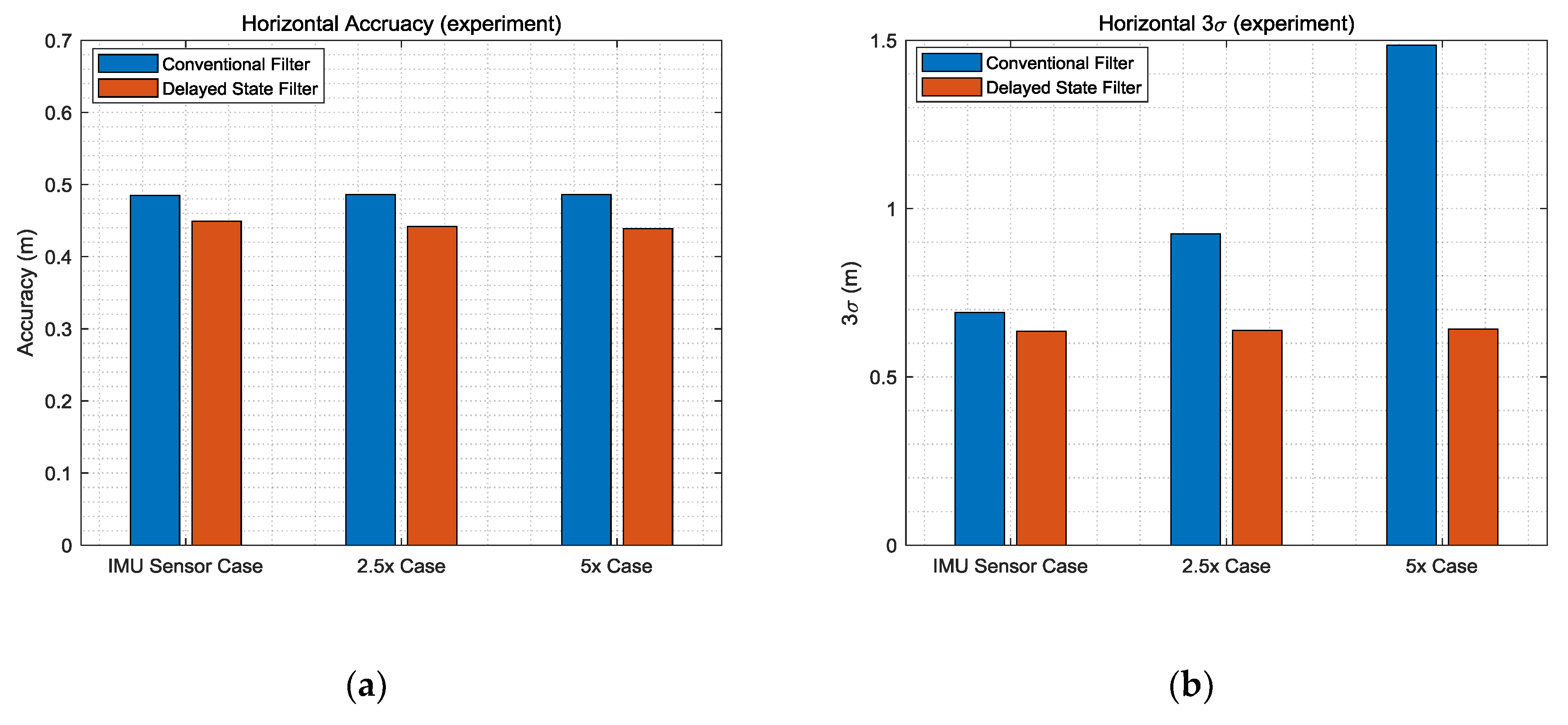
| Meter | IMU Sensor Case | 2.5× Case | 5× Case | |||
|---|---|---|---|---|---|---|
| 3σ | Accuracy | 3σ | Accuracy | 3σ | Accuracy | |
| Conventional Filter | 0.469 m | 0.168 m | 0.779 m | 0.214 m | 1.410 m | 0.274 m |
| Delayed State Filter | 0.384 m | 0.138 m | 0.390 m | 0.139 m | 0.412 m | 0.123 m |
| Time (s) | Conventional Filter | Delayed State Filter |
| Meter | Conventional Filter | Delayed State Filter | ||
|---|---|---|---|---|
| 3σ | Accuracy (RMS 1) | 3σ | Accuracy (RMS 1) | |
| Horizontal | 1.411 m | 0.255 m | 0.417 m | 0.142 m |
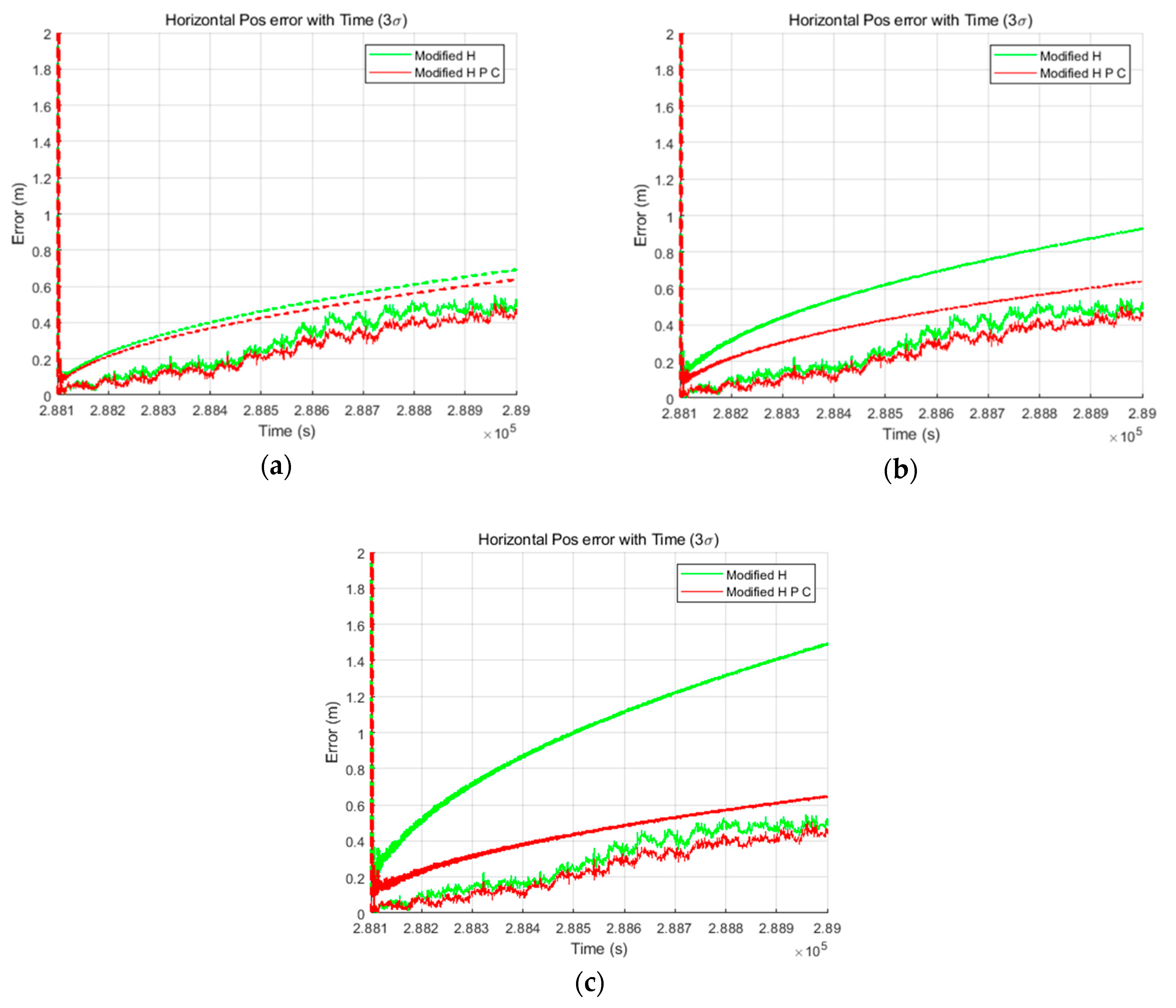
| Meter | IMU Sensor Case | 2.5× Case | 5× Case | |||
|---|---|---|---|---|---|---|
| 3σ | Accuracy | 3σ | Accuracy | 3σ | Accuracy | |
| Conventional Filter | 0.691 m | 0.485 m | 0.925 m | 0.486 m | 1.486 m | 0.486 m |
| Delayed State Filter | 0.636 m | 0.449 m | 0.638 m | 0.442 m | 0.642 m | 0.439 m |
© 2019 by the authors. Licensee MDPI, Basel, Switzerland. This article is an open access article distributed under the terms and conditions of the Creative Commons Attribution (CC BY) license (http://creativecommons.org/licenses/by/4.0/).
Share and Cite
Kim, J.; Kim, Y.; Song, J.; Kim, D.; Park, M.; Kee, C. Performance Improvement of Time-Differenced Carrier Phase Measurement-Based Integrated GPS/INS Considering Noise Correlation. Sensors 2019, 19, 3084. https://doi.org/10.3390/s19143084
Kim J, Kim Y, Song J, Kim D, Park M, Kee C. Performance Improvement of Time-Differenced Carrier Phase Measurement-Based Integrated GPS/INS Considering Noise Correlation. Sensors. 2019; 19(14):3084. https://doi.org/10.3390/s19143084
Chicago/Turabian StyleKim, Jungbeom, Younsil Kim, Junesol Song, Donguk Kim, Minhuck Park, and Changdon Kee. 2019. "Performance Improvement of Time-Differenced Carrier Phase Measurement-Based Integrated GPS/INS Considering Noise Correlation" Sensors 19, no. 14: 3084. https://doi.org/10.3390/s19143084