Physical Extraction and Feature Fusion for Multi-Mode Signals in a Measurement System for Patients in Rehabilitation Exoskeleton

Abstract
:1. Introduction
2. Methods
2.1. Inertial Measurement Unit (IMU)
2.1.1. Overview
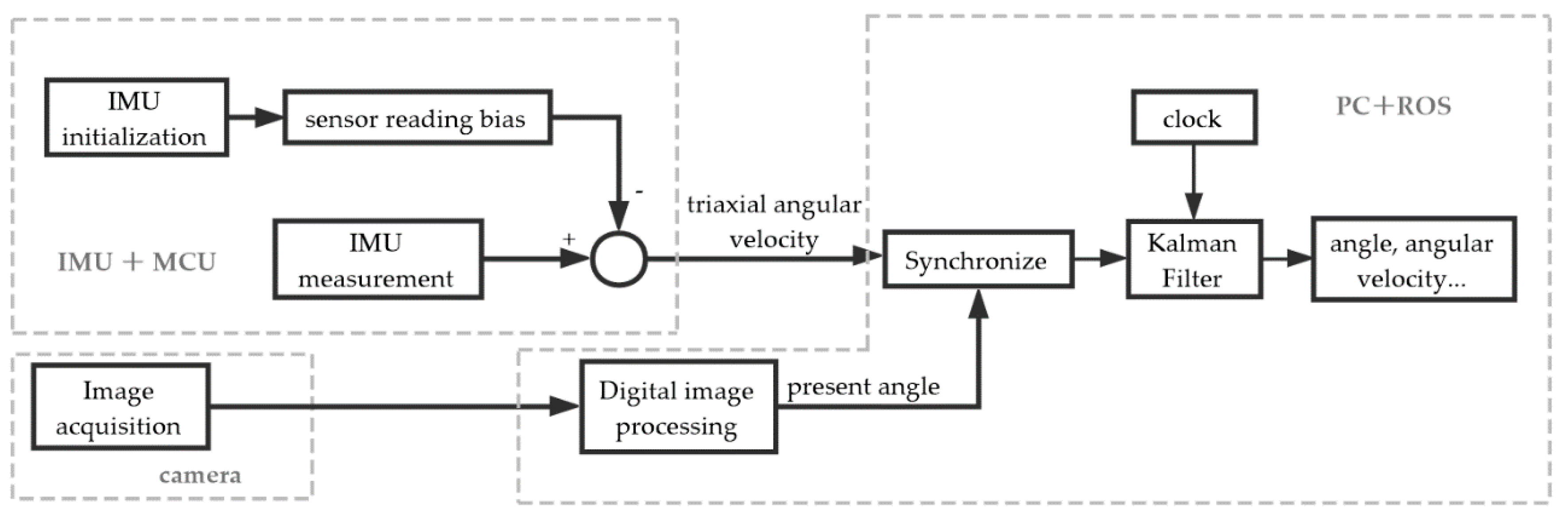
2.1.2. Algorithm
2.1.3. Hardware Implementation
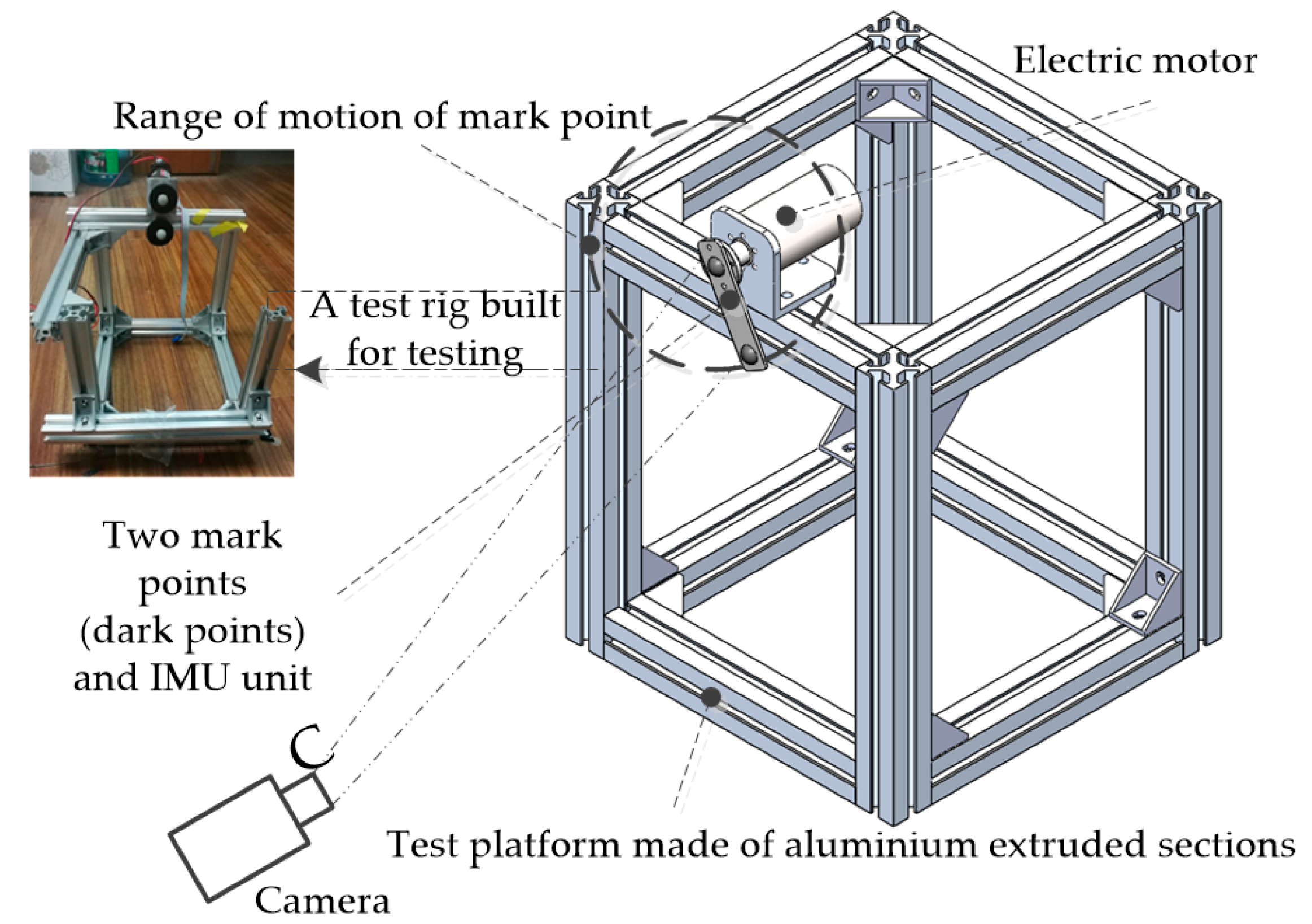
2.2. Visual Measurement Unit (VMU)
2.2.1. Overview
2.2.2. Architecture Implementation
2.3. Data Fusion Unit
2.3.1. Overview
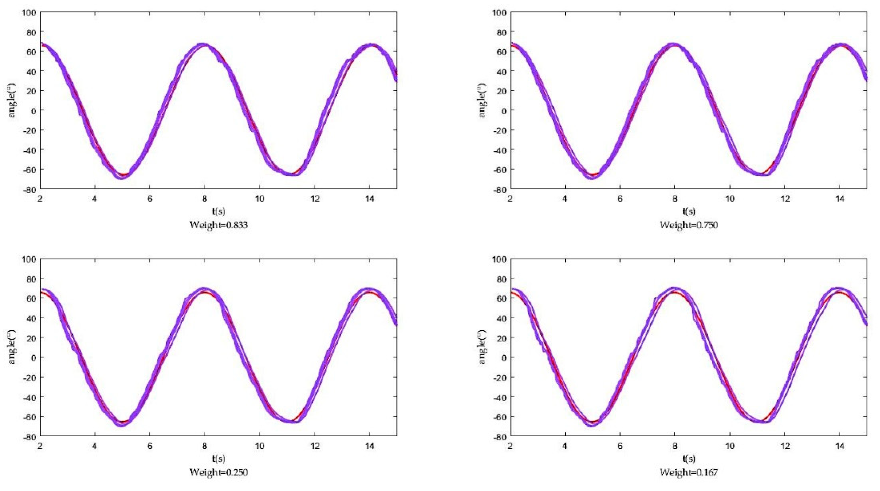
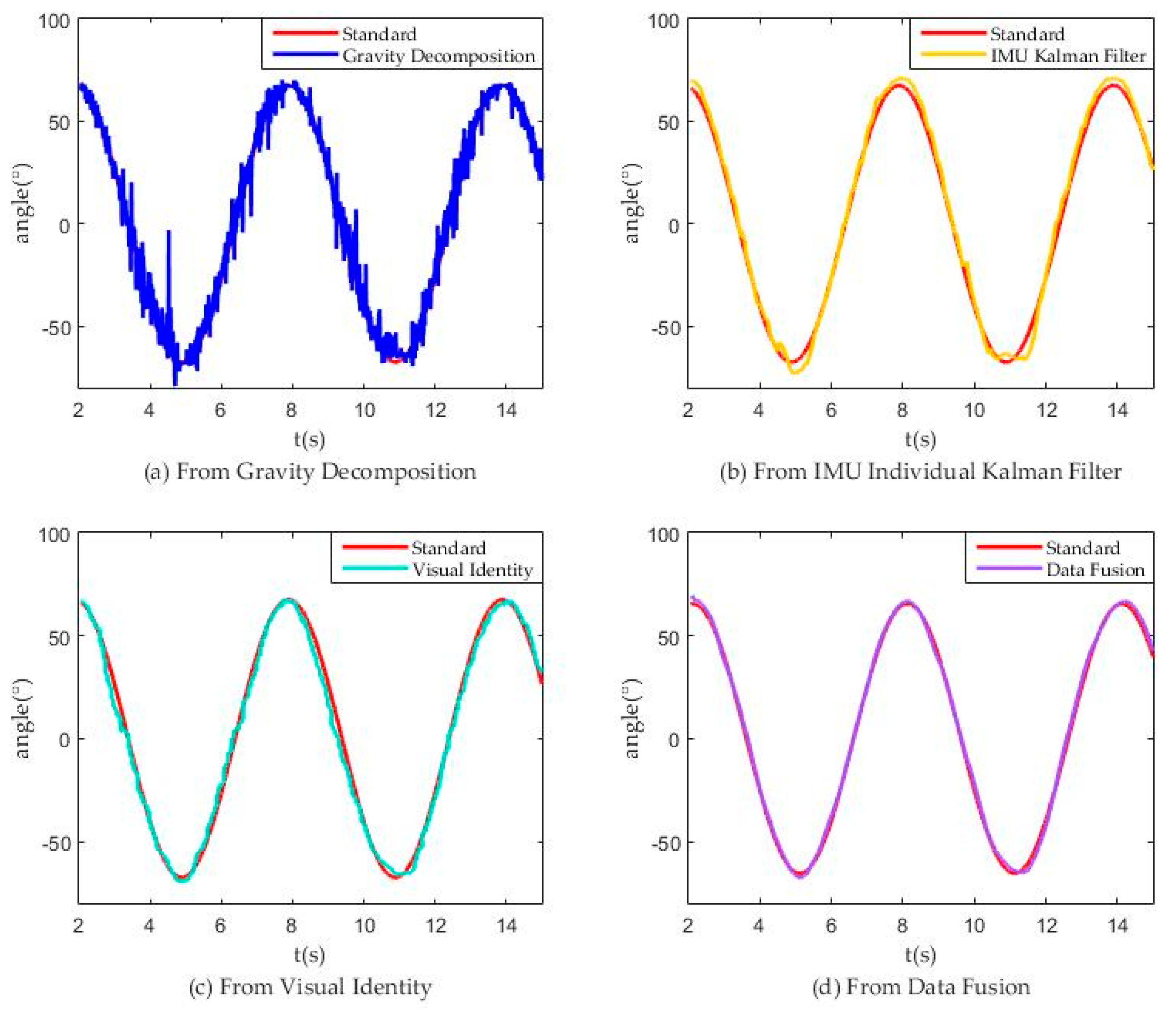
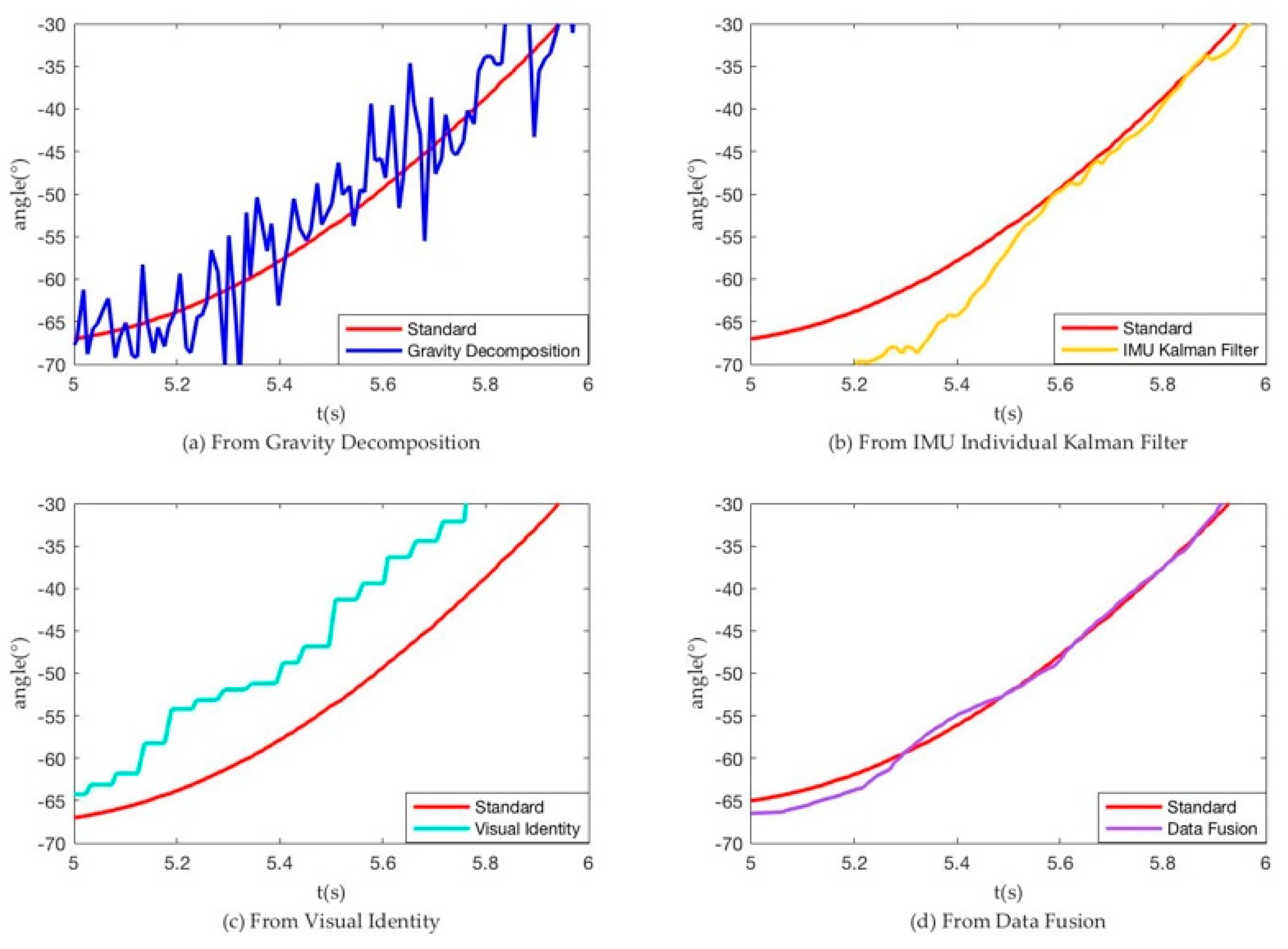
2.3.2. Fusion Algorithm
2.3.3. Proof of Algorithm
3. Tests and Results
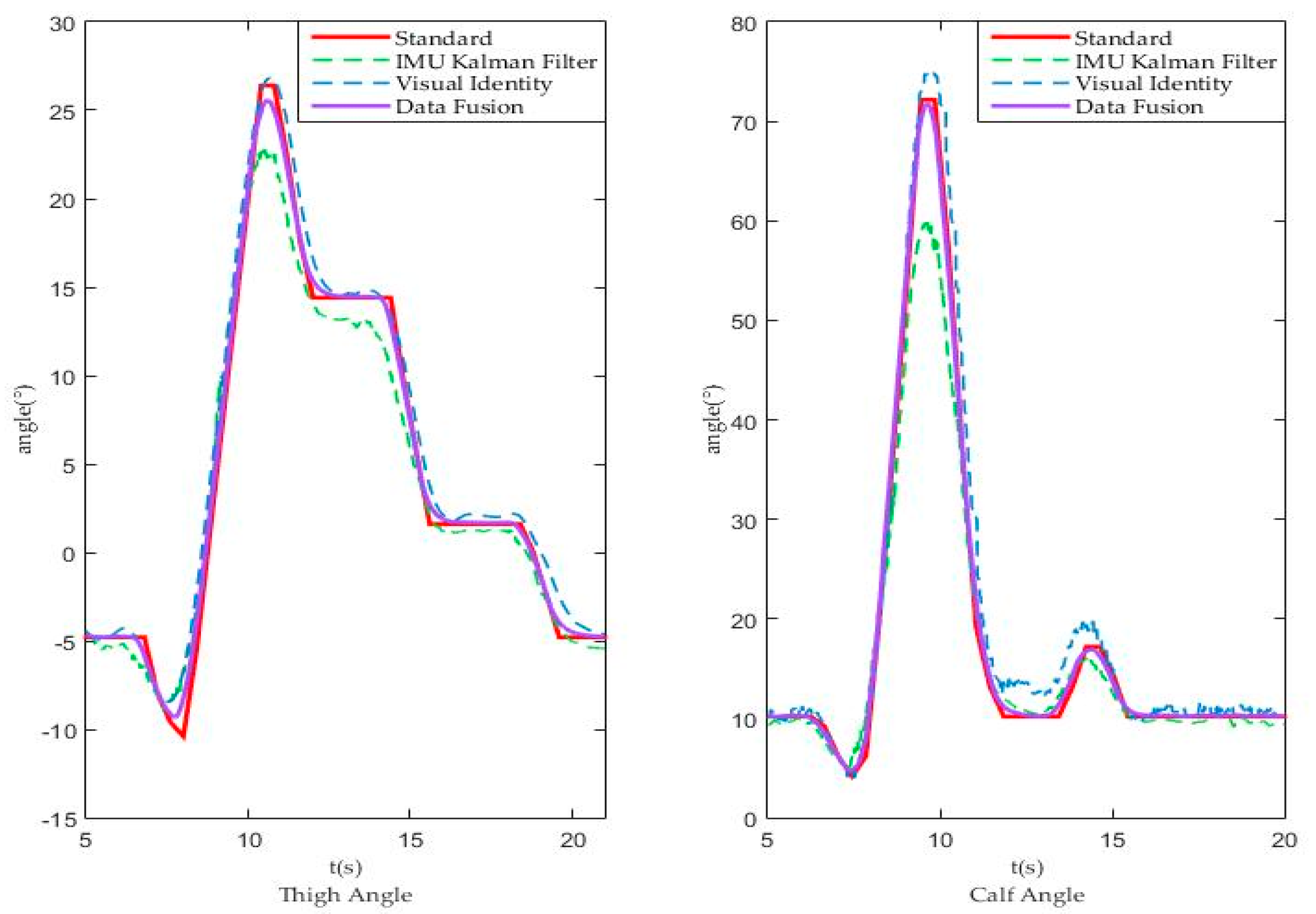
3.1. Exoskeleton Test without Load
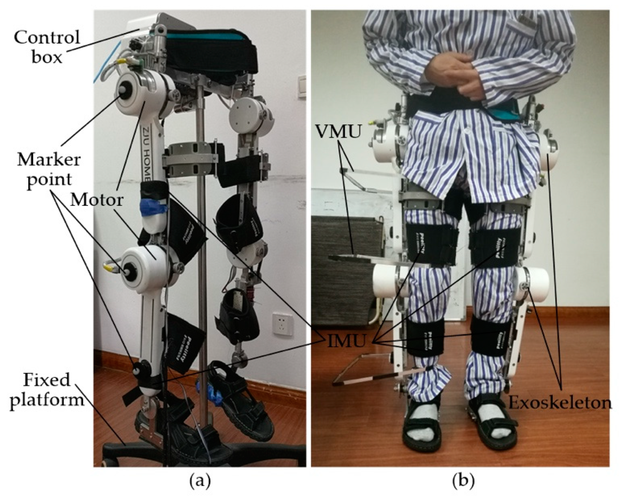
3.2. Human Test with Exoskeleton
4. Discussion and Future Study
Author Contributions
Funding
Acknowledgments
Conflicts of Interest
References
- Taylor, R.H.; Stoianovici, D. Medical robotics in computer-integrated surgery. IEEE Trans. Robot. Autom. 2003, 19, 765–781. [Google Scholar] [CrossRef]
- Han, J.; Lian, S.; Guo, B.; Li, X.; You, A. Active rehabilitation training system for upper limb based on virtual reality. Adv. Mech. Eng. 2017, 12. [Google Scholar] [CrossRef]
- Lim, D.H.; Kim, W.S.; Kim, H.J.; Han, C.S. Development of real-time gait phase detection system for a lower extremity exoskeleton robot. Int. J. Precis. Eng. Manuf. 2017, 18, 681–687. [Google Scholar] [CrossRef]
- Li, J.; Shen, B.; Chew, C.M.; Teo, C.L.; Poo, A.N. Novel Functional Task-Based Gait Assistance Control of Lower Extremity Assistive Device for Level Walking. IEEE Trans. Ind. Electron. 2016, 63, 1096–1106. [Google Scholar] [CrossRef]
- Onen, U.; Botsali, F.M.; Kalyoncu, M.; Tinkir, M.; Yilmaz, N.; Sahin, Y. Design and Actuator Selection of a Lower Extremity Exoskeleton. IEEE/ASME Trans. Mechatron. 2014, 19, 623–632. [Google Scholar] [CrossRef]
- Mancisidor, A.; Zubizarreta, A.; Cabanes, I.; Portillo, E.; Jung, J.H. Virtual Sensors for Advanced Controllers in Rehabilitation Robotics. Sensors 2017, 18, 785. [Google Scholar] [CrossRef] [PubMed]
- Zeilig, G.; Weingarden, H.; Zwecker, M.; Dudkiewicz, I.; Bloch, A.; Esquenazi, A. Safety and tolerance of the ReWalk™ exoskeleton suit for ambulation by people with complete spinal cord injury: A pilot study. J. Spinal Cord Med. 2012, 35, 96–101. [Google Scholar] [CrossRef] [PubMed]
- Kiguchi, K.; Hayashi, Y. An EMG-Based Control for an Upper-Limb Power-Assist Exoskeleton Robot. IEEE Trans. Syst. Man Cybern. Part B Cybern. 2012, 42, 1064–1071. [Google Scholar] [CrossRef] [PubMed]
- Baunsgaard, C.; Nissen, U.; Brust, A.; Frotzler, A.; Ribeill, C.; Kalke, Y.; Biering-Sorensen, F. Gait training after spinal cord injury: Safety, feasibility and gait function following 8 weeks of training with the exoskeletons from Ekso Bionics. Spinal Cord 2018, 56, 106–116. [Google Scholar] [CrossRef] [PubMed]
- Crowley, J.L. Mathematical foundations of navigation and perception for autonomous mobile robot. In Proceedings of the International Workshop on Reasoning with Uncertainty in Robotics, Amsterdam, The Netherlands, 4–6 December 1995. [Google Scholar]
- Park, K.; Chung, D.; Chung, H.; Lee, J.G. Dead Reckoning Navigation of a Mobile Robot Using an Indirect Kalman Filter. In Proceedings of the IEEE International Conference on Multi-Sensor Fusion and Integration for Intelligent Systems, Washington, DC, USA, 8–11 December 1996. [Google Scholar]
- Kalman, R.E. A new approach to linear filtering and prediction problems. J. Basic Eng. 1960, 82, 35–45. [Google Scholar] [CrossRef]
- Welch, G.; Bishop, G. An introduction to the Kalman filter. In Proceedings of the SIGGRAPH, Angeles, CA, USA, 12–17 August 2001; Volume 8, pp. 2759–3175. [Google Scholar]
- Jung, P.G.; Oh, S.; Lim, G.; Kong, K. A Mobile Motion Capture System Based on Inertial Sensors and Smart Shoes. J. Dyn. Syst. Meas. Control 2014, 136, 011002. [Google Scholar] [CrossRef]
- Herda, L.; Fua, P.; Plänkers, R.; Boulic, R.; Thalmann, D. Using Skeleton-Based Tracking to Increase the Reliability of Optical Motion Capture. Hum. Mov. Sci. J. 2001, 20, 313–341. [Google Scholar] [CrossRef]
- Zhang, J.T.; Novak, A.C.; Brouwer, B.; Li, Q. Concurrent validation of Xsens MVN measurement of lower limb joint angular kinematics. Inst. Phys. Eng. Med. 2013, 34, 765–781. [Google Scholar] [CrossRef] [PubMed]
- Li, M.; Zheng, L.; Xu, T.; Wo, H.; Farooq, U.; Tan, W.; Bao, C.; Wang, X.; Dong, S.; Guo, W.; et al. A flexible sensing system capable of sensations imitation and motion monitoring with reliable encapsulation. Sens. Actuators A Phys. 2018, 279, 424–432. [Google Scholar] [CrossRef]
- Mengüç, Y.; Park, Y.L.; Pei, H.; Vogt, D.; Aubin, P.M.; Winchell, E.; Fluke, L.; Stirling, L.; Wood, R.J.; Walsh, C.J. Wearable soft sensing suit for human gait measurement. Int. J. Robot. Res. 2014, 33, 1748–1764. [Google Scholar] [CrossRef]
- Bonato, P. Wearable Sensors and Systems. IEEE Eng. Med. Biol. Mag. 2010, 29, 25–36. [Google Scholar] [CrossRef] [PubMed]
- Zhang, W.; Tomizuka, M.; Byl, N. A Wireless Human Motion Monitoring System Based on Joint Angle Sensors and Smart Shoes. ASME J. Dyn. Syst. Meas. Control 2016, 138, 111004. [Google Scholar] [CrossRef]
- Pan, M.; Wood, E.F. Data assimilation for estimating the terrestrial water budget using a constrained ensemble Kalman filter. J. Hydrometeorol. 2006, 7, 534–547. [Google Scholar] [CrossRef]
- Grosu, V.; Grosu, S.; Vanderborght, B.; Lefeber, D.; Rodriguez-Guerrero, C. Multi-Axis Force Sensor for Human–Robot Interaction Sensing in a Rehabilitation Robotic Device. Sensors 2017, 17, 1294. [Google Scholar] [CrossRef] [PubMed]
- Moore, T.; Stouch, D. A Generalized Extended Kalman Filter Implementation for the Robot Operating System. Adv. Intell. Syst. Comput. 2015, 302, 335–348. [Google Scholar] [CrossRef]
- Yang, W.; Yang, C.J.; Xu, T. Human hip joint center analysis for biomechanical design of a hip joint exoskeleton. Front. Inf. Technol. Electron. Eng. 2016, 17, 792–802. [Google Scholar] [CrossRef]
- Hall, D.L.; Llinas, J. An introduction to multi-sensor data fusion. Proc. IEEE 1997, 1, 6–23. [Google Scholar] [CrossRef]
- Dong, J.; Zhuang, D.; Huang, Y.; Fu, J. Advances in Multi-Sensor Data Fusion: Algorithms and Applications. Sensors 2009, 9, 7771–7784. [Google Scholar] [CrossRef] [PubMed] [Green Version]


| Practical Angle (°) | Measurement Angle (°) | Relative Error (%) |
|---|---|---|
| 0 | 0.69 | / |
| 15 | 15.44 | 2.93 |
| 30 | 30.24 | 0.8 |
| 45 | 45.12 | 0.27 |
| 60 | 60.12 | 0.2 |
| 75 | 75.08 | 0.11 |
| 90 | 89.65 | 0.39 |
© 2018 by the authors. Licensee MDPI, Basel, Switzerland. This article is an open access article distributed under the terms and conditions of the Creative Commons Attribution (CC BY) license (http://creativecommons.org/licenses/by/4.0/).
Share and Cite
Yang, C.; Wei, Q.; Wu, X.; Ma, Z.; Chen, Q.; Wang, X.; Wang, H.; Fan, W. Physical Extraction and Feature Fusion for Multi-Mode Signals in a Measurement System for Patients in Rehabilitation Exoskeleton. Sensors 2018, 18, 2588. https://doi.org/10.3390/s18082588
Yang C, Wei Q, Wu X, Ma Z, Chen Q, Wang X, Wang H, Fan W. Physical Extraction and Feature Fusion for Multi-Mode Signals in a Measurement System for Patients in Rehabilitation Exoskeleton. Sensors. 2018; 18(8):2588. https://doi.org/10.3390/s18082588
Chicago/Turabian StyleYang, Canjun, Qianxiao Wei, Xin Wu, Zhangyi Ma, Qiaoling Chen, Xin Wang, Hansong Wang, and Wu Fan. 2018. "Physical Extraction and Feature Fusion for Multi-Mode Signals in a Measurement System for Patients in Rehabilitation Exoskeleton" Sensors 18, no. 8: 2588. https://doi.org/10.3390/s18082588