Attention-Based Recurrent Temporal Restricted Boltzmann Machine for Radar High Resolution Range Profile Sequence Recognition


College of Electronic Science, National University of Defense Technology, Changsha 410073, China
*
Author to whom correspondence should be addressed.
Sensors 2018, 18(5), 1585; https://doi.org/10.3390/s18051585
Submission received: 30 March 2018
/
Revised: 13 May 2018
/
Accepted: 14 May 2018
/
Published: 16 May 2018
(This article belongs to the Section Remote Sensors)
Abstract
:The High Resolution Range Profile (HRRP) recognition has attracted great concern in the field of Radar Automatic Target Recognition (RATR). However, traditional HRRP recognition methods failed to model high dimensional sequential data efficiently and have a poor anti-noise ability. To deal with these problems, a novel stochastic neural network model named Attention-based Recurrent Temporal Restricted Boltzmann Machine (ARTRBM) is proposed in this paper. RTRBM is utilized to extract discriminative features and the attention mechanism is adopted to select major features. RTRBM is efficient to model high dimensional HRRP sequences because it can extract the information of temporal and spatial correlation between adjacent HRRPs. The attention mechanism is used in sequential data recognition tasks including machine translation and relation classification, which makes the model pay more attention to the major features of recognition. Therefore, the combination of RTRBM and the attention mechanism makes our model effective for extracting more internal related features and choose the important parts of the extracted features. Additionally, the model performs well with the noise corrupted HRRP data. Experimental results on the Moving and Stationary Target Acquisition and Recognition (MSTAR) dataset show that our proposed model outperforms other traditional methods, which indicates that ARTRBM extracts, selects, and utilizes the correlation information between adjacent HRRPs effectively and is suitable for high dimensional data or noise corrupted data.
1. Introduction
A high-resolution range profile (HRRP) is the amplitude of the coherent summations of the complex time returns from target scatters in each range cell, which represents the projection of the complex returned echoes from the target scattering centers on to the radar line-of-sight (LOS) [1]. The HRRP recognition has been studied for decades in the field of RATR because it contains important structural information such as the target size and the distribution of scattering points [1,2,3,4]. In addition, the HRRP is easy to obtain, store, and process. For the problem of HRRP recognition, a large number of scholars have conducted extensive research [1,5,6,7]. The reported methods can be summarized as extracted features of HRRPs after dividing the full target radar aspect angles into several frames and performing the target detection to select the region of interest in an HRRP. The difference between these methods lies in feature extraction. Common feature extraction techniques include HRRP templates, HRRP stochastic modeling, time-frequency transform features, and invariant features [8,9]. These feature extraction techniques all have clear physical meaning and are conducive for promotion. However, most traditional recognition methods utilize the single HRRP rather than HRRP sequences, which ignores the temporal and spatial correlation within the sample.
Noting strong relativity is contained between the adjacent HRRP, sequential HRRP is of potential usage for recognition. To make use of the spatial and temporal correlation in a sequence, HMM is often utilized for sequential problems such as sequential event detection in wireless sensor networks and radar HRRP sequence recognition [10,11]. This method utilizes the sequence information of HRRP and considers the structure information inside the target. In addition, the problem of azimuth sensitivity is solved by framing [12,13,14]. However, the model can only represent local dependencies between states and has a high computational complexity, which means it is not efficient at dealing with high dimensional sequential data. Recently, deep learning has been gradually applied to radar. Ahmet Elbir constructed a CNN model as a multi-class classification framework to select antennas in a cognitive radar scenario, which is an essential application of deep learning in the radar field [15]. However, the provided method still does not consider the situation of high dimensional sequential data.
Dealing with high dimensional sequential data has also been widely studied in the machine learning community. Recently, a time-series model, which is potentially better studied to capture dependency structures, relies on the use of Recurrent Neural Networks (RNNs). However, there are many parameters that need to be trained in the model, which leads to the problem of gradient dissipation or gradient explosion in the training process [16]. The Residual Network (ResNet) can effectively solve the problem of gradient dissipation or gradient explosion by sharing the cross layer parameter and retaining the intermediate features [17]. However, the model has no obvious advantages in the processing of sequential data. Following the invention of the fast learning algorithm named contrastive divergence algorithm (CD) [18] and its successful application to Restricted Boltzmann Machine (RBM) learning, the Recurrent Temporal Restricted Boltzmann Machine (RTRBM) has been proposed as a generative model for high dimensional sequences [19,20,21,22,23,24]. More specifically, the RTRBM model is constructed by rolling multiple RBMs over time [21] where each RBM has a contextual hidden state that is received from the previous RBM and is used to modulate its hidden units. Add to it, RBM is a bipartite graphical model that uses a layer of “hidden” binary variables or units to model the probability distribution of a layer of “visible” variables [24,25,26,27,28]. Based on this, the RTRBM model introduces the correlation matrix between the hidden layers of adjacent RBMs to tack the correlation inside the data into consideration [19]. The model has achieved great success in extracting internal correlations between adjacent HRRPs and capturing spatial and temporal patterns in highly dimensional sequential data. In the traditional method based on RTRBM, only one hidden layer (at time frame t) is utilized for the recognition. However, in the training process of the RTRBM model, the gradient of the parameters is propagating with time series, the ‘vanishing gradient problem’ appears easily when T becomes longer. Therefore, with the time series propagating, the model cannot extract deeper features and the sequential correlation features cannot transmit to the next RBM smoothly in the learning process. As such, it is necessary to consider feature vectors at all the T time sequences. Considering that the contribution of each feature vector to the recognition is different and has been ignored in the traditional method based on RTRBM, it is essential for the recognition method to gain the ability to pay more attention to the important feature parts.
In order to solve the problems which have been put forward, a new method that combines the RTRBM model with the attention mechanism [29] for sequential radar HRRP recognition is proposed in this paper. The attention mechanism was first proposed in the field of the visual image in Reference [30] and has shown good performance on a range of tasks including machine translation, machine comprehension, and Relation classification [31,32,33,34,35,36]. Therefore, it is theoretically possible for HRRP sequence recognition when utilizing the attention mechanism. In ARTRBM, the combination of RTRBM and the attention mechanism makes the model focus its attention on specific features, which are important for the classification task. More specifically, this model encodes the HRRPs sequence through the RTRBM model and then calculates the weight coefficient for each hidden unit, according to their contributions to the recognition performance. Then the features are utilized to construct the attention layer for the recognition task. This combination brings performance improvements for high recognition accuracy achievement and strong robustness to noise. To verify the effectiveness of the proposed model, two experiments are executed, which utilizes the HRRP data converted from the SAR data of MSTAR [37]. Experimental results indicate the superior performance of the proposed model against HMM, Class RBM, and Principle Component Analysis (PCA). Additionally, the proposed model can still achieve an ideal accuracy when the intensity of noise is lower than −15, which confirms its strong robustness to noise.
This paper is organized as follows. In Section 2, the RBM and RTRBM are briefly introduced as a preparation for the proposal of the method. In Section 3, the proposed model for sequential HRRP recognition is presented in detail, which is followed by the training method for the proposed model in Section 4. After that, several experiments on the MSTAR dataset have been performed to evaluate our model in Section 5. Lastly, we conclude our work in Section 6.
2. Preliminaries
In this section, we will go over the salient properties of the Restricted Boltzmann Machine (RBM) briefly and then give preliminaries about Recurrent Temporal Restricted Boltzmann Machine (RTRBM), which is a temporal extension of RBMs.
2.1. Restricted Boltzmann Machine
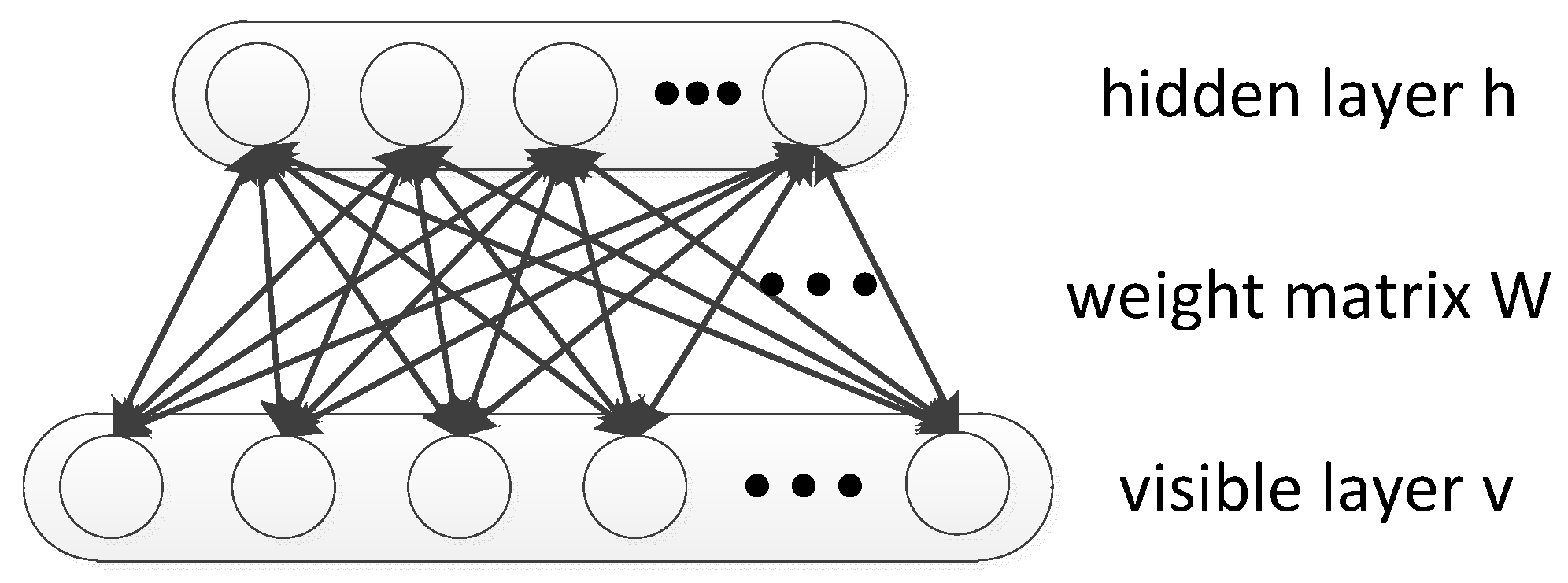
The RBM is an undirected graphical model that uses a layer of hidden variables to model a joint distribution over the visible variables [16]. The graphical depiction of the RBM is depicted in Figure 1. The two layers are fully connected to each other by a weight matrix W but there exists no connections between units within the same layer [28,38]. On the problem of HRRP-based RATR, visible units can be an HRRP sample and the hidden layer can be used to extract the features.
The RBM defines the joint distribution over visible units and hidden units , which is shown in the equation below [24].
where is the partition function, which is given by adding all possible pairs of visible and hidden vectors. Additionally, E is an energy function defined below.
where consists of the model parameters, represent the weight matrix connecting visible and hidden vectors, and and are the biases of the visible and hidden layers, respectively.
2.2. Recurrent Temporal Restricted Boltzmann Machine
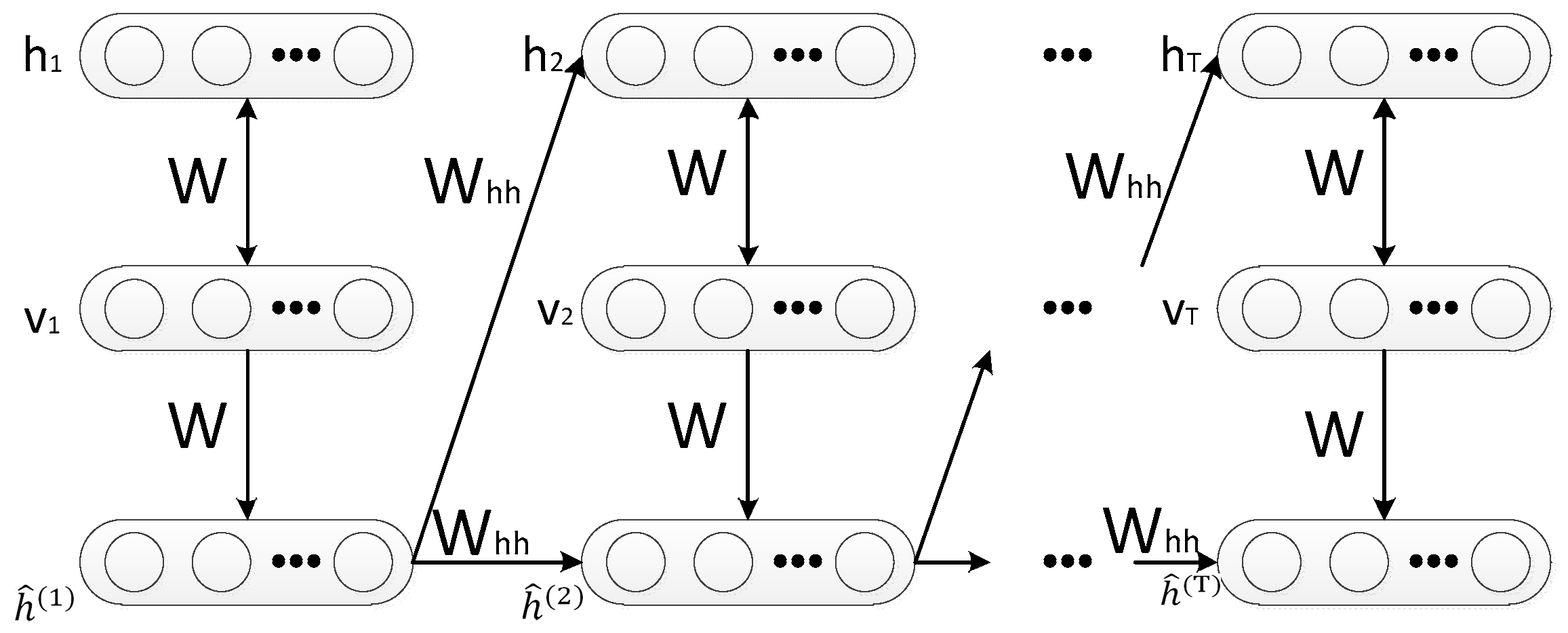
The Recurrent Temporal Restricted Boltzmann Machine is a generative model for modeling high-dimensional sequences, which was constructed by rolling multiple RBMs over time. In detail, the RBM at time step t is connected at t − 1 through the weight matrix and is conditioned on it. The dependency on is the major difference compared to the RBM. It is worth noting that this horizontal deep architecture is different from the Deep Brief Networks (DBN), which stacks RBMs vertically [39]. Therefore, more sequence information can be extracted by RTRBM and performs better in many application scenarios such as radar HRRP target recognition.
The graphical model for the RTRBM is illustrated in Figure 2.
The model gives five parameters . Here W is the weight matrix between the visible and the hidden layer of the RBM at each time frame. stands for the directed weights, which connect the hidden layer at time t – 1 and t, and is a vector of initial mean-file values of the hidden units. The motivation for the choice of is that, using the RBM associated with time instant t, we have that ; i.e., it is the expected value of the hidden units vector. In addition, and are the biases of visible and hidden layers. respectively. In RTRBM, the RBM at time frame t is conditioned on itself at time step t − 1 through a set of time dependent model parameters such as the visible and hidden layer biases and that depend on [40].
while is the mean-filed value of , which is represented in detail below.
Given hidden inputs (t > 1), the conditional distributions are factorized and takes the form below.
Therefore, the joint probability distribution of the visible and hidden units of the RTRBM with length T takes the form below [21].
where denotes the normalization factors for the RBM at T = t and is the energy function at the time step t, which is defined by the equation below.
Furthermore, given the hidden inputs , all the RBMs are decoupled. Therefore, sampling can be performed using block Gibbs sampling for each RBM independently. This fact is useful in deriving the CD algorithm, which is a stochastic approximation and utilizes a few Gibbs sampling steps to estimate the gradient of parameters [18,41].
3. The Proposed Model
Based on the original RTRBM, the newly proposed model brings the idea of the attention mechanism, which is named Attention based RTRBM. The graphical structure of the proposed model is demonstrated in Figure 3. In the proposed model, RTRBM is utilized to extract features from the input data and store the extracted features in the hidden vector. A new hidden layer is introduced to RTRBM by the weighted sum in all hidden layers for the reason of measuring the role of each hidden vector in recognition tasks and then the new hidden layer is used for classification.
In the context of radar HRRP recognition, the input data is the raw HRRPs sequence and the output y is a sequence of the class label. Each feature vector is extracted from the RTRBM, which is treated as an encoder to form a sequential representation.
The upper half of Figure 3 represents the attention mechanism in the ARTRBM model. The fundamental principle of the attention mechanism can be expressed as the classifier paying more attention to the major part rather than all the extracted feature vectors.
As is shown in Figure 3, stands for the weight coefficient for the hidden layer at time step t. The layer is determined by the hidden layer of each time step and corresponds to the weight matrix, which connects the layer s and output layer y. Additionally, y is a vector representing the class label in which all values are set to 0 except at the position corresponding to a label y, which is set to 1.
In order to detail and describe the process of our model, the flowchart about ARTRBM is shown below.
As shown in Figure 4, the basic process of the attention mechanism can be summarized in three steps. First, computing the feature energy and weight coefficients which represent the contribution of extracted feature vectors for recognition. Afterward, the final hidden layer s is constructed, which is determined by the hidden layers of all time steps. Finally, the layer s is used in the final classification task.
In the attention mechanism, the final feature vector is obtained by the weighted summation of the hidden layers of each time, which can be expressed in the equation below.
where the weight coefficient can be defined as:
where represents the vector of the jth row elements of the matrix and corresponds to the hidden layer energy at time frame j. The weight coefficient represents the role of the hidden layer feature in recognition. The attention mechanism [30,41,42] is also determined by the parameter . By training the parameters and , the model can assign the hidden layer with different weights at different moments, which makes the model more focused on the parts that play a major role in the recognition tasks.
4. Learning the Parameters of the Model
In the proposed model, the RTRBM plays a role of the encoder, which describes the joint probability distribution . According to Equation (3) and Equation (7), the energy function can be computed and is shown below.
In order to learn the parameters, first, we need to obtain the partial derivatives of with respect to the parameters. We use CD approximation [15,17] to compute these derivatives, which require the gradients of energy function (10) to be based on all the model parameters. Afterward, we separate the energy function into the following two terms , where:
Therefore, the gradients of representing the parameters were separated into two parts. It is straightforward to calculate the gradients of , and calculating would be more complex. To compute , we first compute , which can be computed recursively using the back propagation-through-time (BPTT) algorithm (David Rumelhart, Geoffrey Hinton et al., 1986) and the chain rule. Therefore, the model parameters can be updated via gradient ascent, which is shown in the equation below.
where represents the universal mean of the gradient function under the conditional probability and can be expressed using the equation below.
Therefore, Equation (12) can be derived as:
Specifically, and are shown in Appendix A.
We extract the features from the input data with the RTRBM model, which are stored in at every time step. Then we use as the input for the attention mechanism and compute the final hidden layer s using Equation (8). To learn the parameters of the attention mechanism, we need to choose an appropriate objective function. Here we use a close variant of perplexity known as cross entropy, which represents the divergence between the entropy calculated from the predicted distribution and that of the correct prediction label (and can be interpreted as the distance between these two distributions). It can be computed using all the units of the layer and expressed as:
where is the set of training examples, n represents the serial number of the training sample, and is the final hidden layer while corresponds to the target labels. By taking Equations (8) and (9) into the objective function (15), the gradient can be calculated and is derived below.
where:
and:
with:
where y and denotes the correct label and the output label, respectively. is the weight matrix that connects layer and label vector y while the logic function is applied to each element of the argued vector. Therefore, the gradients can be exactly computed. The brief deduction process and results are show in Appendix B.
The pseudo code of the model parameter update for the proposed model is summarized in Algorithm 1, which is shown below.
| Algorithm 1. Pseudo code for the learning steps of Attention based RTRBM model |
| Input: training pair: {v_train; y_train}, hidden layer size: dim_h; |
| learning rate: ; momentum: ; and weightcost: . |
| Output: label vector y |
| # Section 1: Extract features using RTRBM |
| (1): Calculate according to Equation (4). |
| (2): Calculate and respectively, |
| according to Equation (5). |
| (3): Calculate the L2 reconstruction error: . |
| (4): Update parameters of this section: , |
| (5): Repeat step (1) to (4) for 1000 epochs and save the trained for test phase. |
| # Section 2: Classification with Attention mechanism |
| (1): Calculate according to Equation (9). |
| (2): Calculate according to Equation (8). |
| (3): Calculate the cross entropy according to Equation (15). |
| (4): Update parameters of this section: |
| (5): Repeat step (1) to (4) for 1000 epochs and save the trained for the test phase. |
5. Experiments
In order to evaluate the proposed recognition model, several experiments on the MSTAR dataset have been presented. First, arranging the training and testing HRRP sequences was introduced in Section 5.1. Afterward, we completed two experiments with different purposes in Section 5.2. The first section compared the performance of our proposed model with several other comparative models and the second section tested the recognition ability of our model with different noise intensities.
5.1. The Dataset
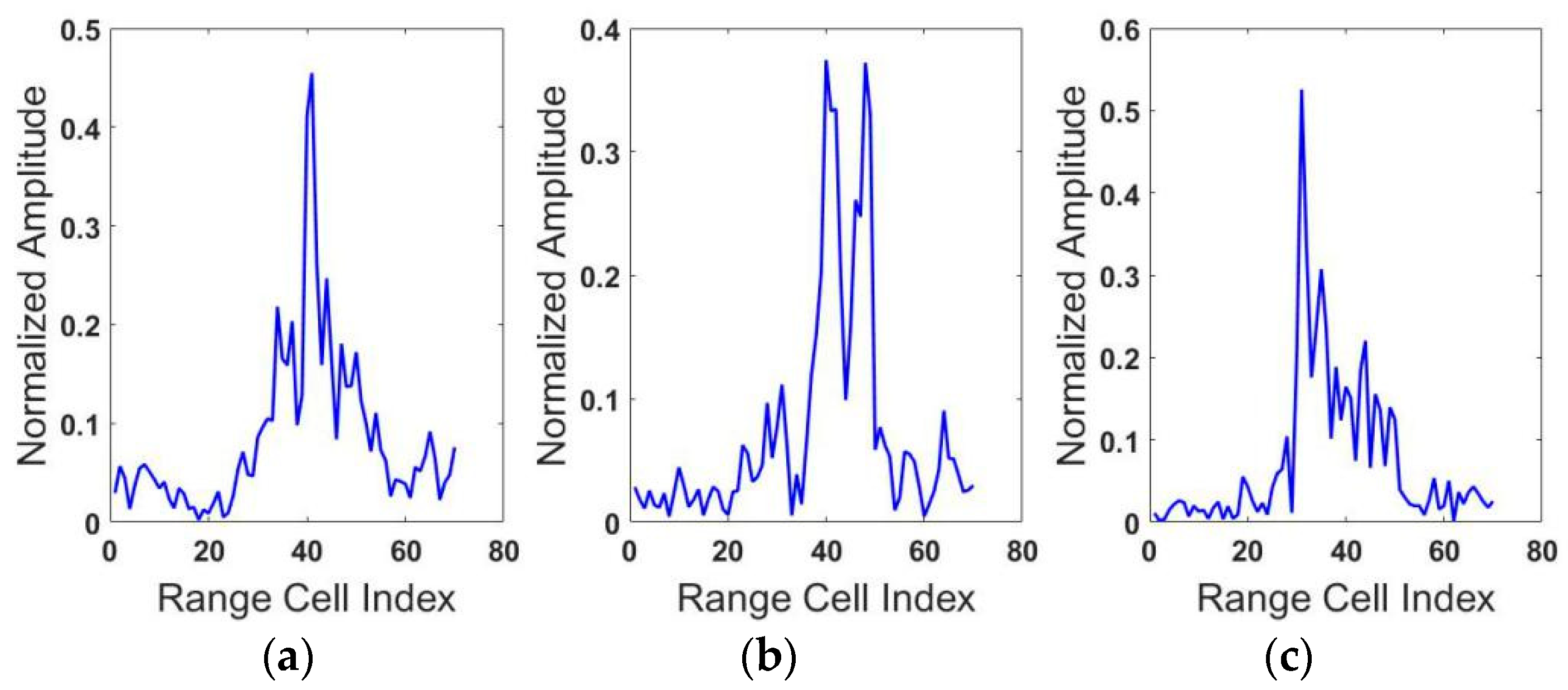
In order to show the clear comparisons between our results with those in other papers more easily, the publicly-available MSTAR (Moving and Stationary Target Acquisition and Recognition) dataset, which has been widely used in related research was chosen in our experiments [12]. MSTAR is funded by DARPA and is the standard dataset of the SAR automatic target recognition algorithm. More detailed, the MASTAR dataset includes 10 kinds of targets data (X band) under different azimuth angles and we chose three of the most similar targets for the experiment, which are the T72 main battle tank, the BMP2 armored personal carrier, and the BTR70 armored personal carrier. In order to make the MSTAR dataset suitable for our model, we first transformed the two-dimensional SAR into a one-dimensional HRRP vector to train our proposed model. The HRRP of the three targets are shown in Figure 5.
All three classes of targets cover 0 to 360 degrees of aspect angles and their distance and azimuth resolutions are 0.3 m [43,44]. In the dataset, each target is obtained under the depression angle of 15° and 17°. The HRRPs of 17 degree of depression angle were used as the training data while the HRRPs of 15° were used as the test data. The size of the training and testing dataset is briefly illustrated in Table 1.
We can see from the table that there are three targets in the table. The targets BMP2 and T72 contain three similar models, respectively, while BTR70 contains one model. Taking BMP2 as an example, we use Sn_C9563 to train the ARTRBM model and test it with Sn_C9563, Sn_C9566, and Sn_C21. In this way, the generalization performance of our model can be examined. The training set and testing set contain 6980 HRRPs and 13,650 HRRPs, respectively.
We divided the 360° of aspect angles into 50 aspect frames uniformly. Each frame covers 7.2°. In each frame, an HRRP is sampled at intervals of 0.1 degrees. Therefore, each frame contains 72 HRRPs. Additionally, the composition of the sequential HRRP datasets is shown in Figure 6.
To make the process more clearly, suppose that each HRRP sequence contains HRRPs and the steps to construct the sequential HRRP are shown as Algorithm 2 [45].
| Algorithm 2. The composition of the sequential HRRP datasets. |
| Step 1: Start from the aspect frame 1 to L. The first HRRPs in frame 1 to L are chosen to form the first HRRP sequence with length L. Slide one HRRP to the right and the second HRRPs in aspect frame 1 to L are chosen to form the second HRRP sequence. Repeat this algorithm until the end of each frame. |
| Step 2: Slide one frame to the right and repeat step 1 to construct the following sequences. |
| Step 3: Repeat step 2 until the end of all aspect frames. If the remaining frame is less than L, then the first frames are cyclically used one by one to form the remaining sequences. |
In many studies, the clutter is removed to get “clean” HRRPs. We directly used the raw HRRPs. The only preprocessing was normalizing the magnitude of each HRRP to its total energy. This setting could make the experiments more closed to real recognition scenarios.
5.2. Experiments
5.2.1. Experiment 1: Investigating the Influence of Hidden Layer Size on Recognition Performance
In this experiment, we will investigate the influence of the size of the hidden layer on recognition performance. In order to explore this problem, two groups of contrastive experiments were organized for different purposes. The first group is aimed at comparing the performance of the Attention-based RTRBM model with contrast models on different hidden layer sizes while the second is to investigate whether the attention mechanism really works and how much effect it has on performance.
Before conducting the experiments, we analyzed the influence rising from the length of the RTRBM model at first. According to Table 2, it shows that when T is increased by more than 15, stable test accuracy can be achieved. In addition, we can further improve the recognition rate by adding hidden units. Therefore, to seek a balance between recognition accuracy and computational complexity, T = 15 is adopted for the recognition task.
(A) Comparing the Performance of the Proposed Model with the Traditional Models
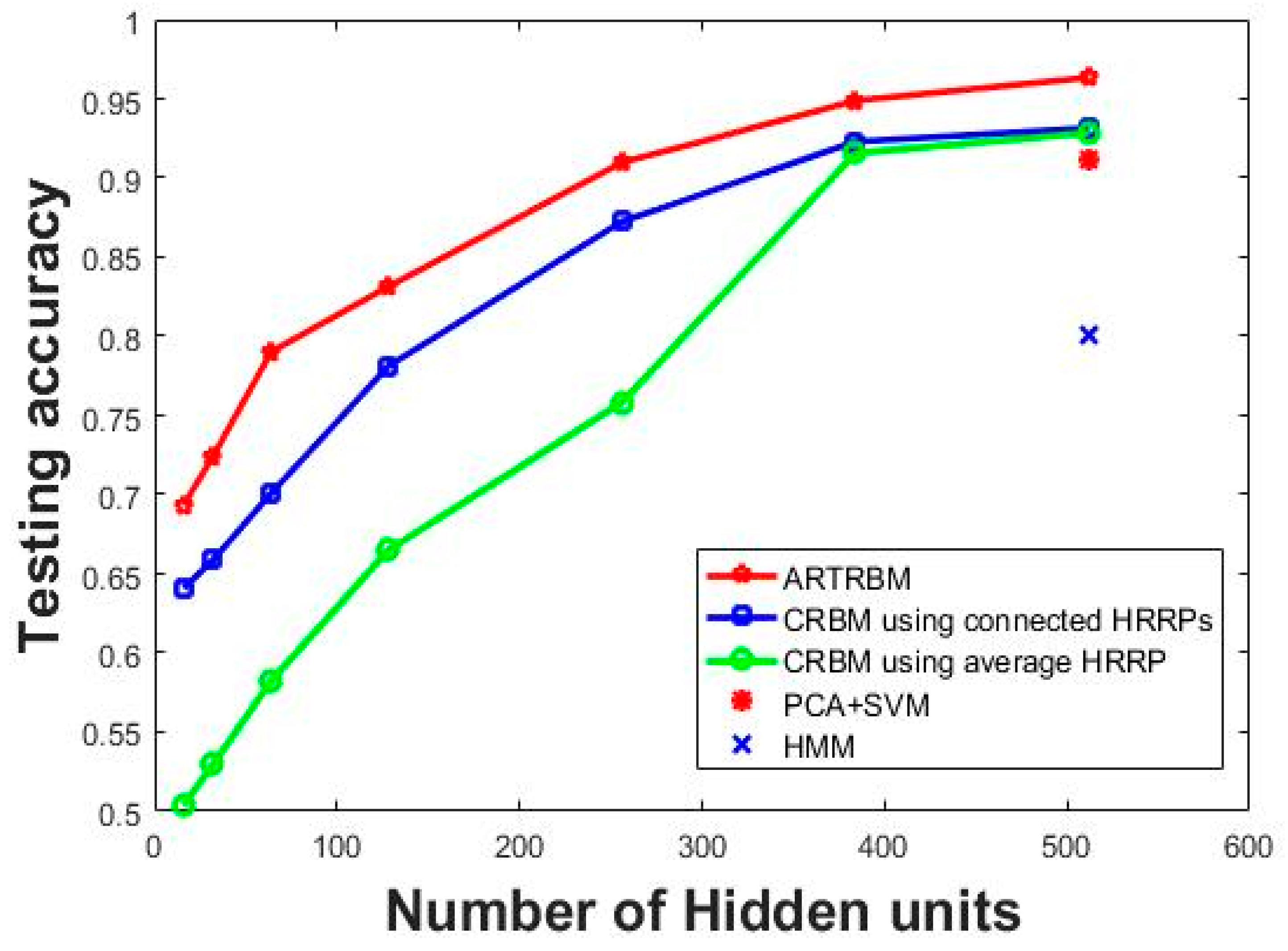
In the first group of contrast experiment, Class RBM (CRBM) with different hidden layer sizes (number of hidden nodes = 16, 32, 64, 128, 256, 384, 512) were trained as comparisons to the proposed method. We carry out the contrast experiments with two different data input methods by constructing an average HRRP with 15 adjacent HRRPs and connecting 15 HRRPs end-to-end. The recognition performance of each model is shown in Figure 7 where the test accuracy is computed by averaging the test results of the three targets.
It can be seen in Figure 7 that the superior recognition performance of Attention-based RTRBM against the other two models. Additionally, our proposed model gets optimal recognition accuracy on each size of the hidden layer, which shows the strong ability to deal with high dimensional sequences. The explanation for this result is that the proposed model can extract more separable features through the RTRBM model and make better use of them using the attention mechanism. Class RBM with average HRRP performs not as good as the other two models, but gets ideal recognition accuracy when the number of hidden nodes increased to 384, which reflects that Class RBM needs more hidden units to reach high recognition accuracy.
We design another baseline using PCA to reduce the dimension of input data. There are 15 features retained after PCA and the classifier is the Support Vector Machine (SVM). We repeat the baseline five times and the average test accuracy is 91.22%. Since the contrast experiment PCA+SVM does not contain hidden units, we mark the results of the model at 512 hidden units in Figure 7. Therefore, we can compare the PCA+SVM model with the best results of other methods. Additionally, the test performance of the HMM model is lower than 80% when the sequence length is 15, which is provided by Reference [12]. Similarly, we mark the results HMM at 512 hidden units in Figure 7 to compare with the best results of other methods. Then we can conclude from Figure 7 that the correlation matrix between the adjacent hidden layers helps RTRBM to extract more discriminatory features and the weight coefficients make the attention mechanism select more separable features, which means that ARTRBM is more suitable for the radar HRRP sequence recognition task.
To gain insight into the performance of three methods on different targets, we list the confusion matrix for the three targets in Table 3. The number of hidden units for all the methods is 384.
As shown in Table 3, the misclassification of BMP2 lowers the average accuracy. One possible reason is that the features learned by the three models are not discriminatory enough to recognize the true targets and another reason may be summarized as we train the models only on BMP2 (Sn_C9563). However, test models on three types of the targets BMP2 and the three types of BMP2 (shown in Figure 8) has a low similarity, which is lower than the three types of T72. However, our proposed model still achieves higher accuracy than two contrast models on the classification of BMP2, which indicates that Attention-based RTRBM is a better choice when there is a great difference between the training and testing dataset.
(B) Evaluating the Impact of Attention Mechanism on Recognition Performance
In the second contrastive experiments group, we designed several ways in which, without attention mechanism, we complete the comparison. In addition, the purpose is to investigate the impact of attention, which is the mechanism in the recognition performance.
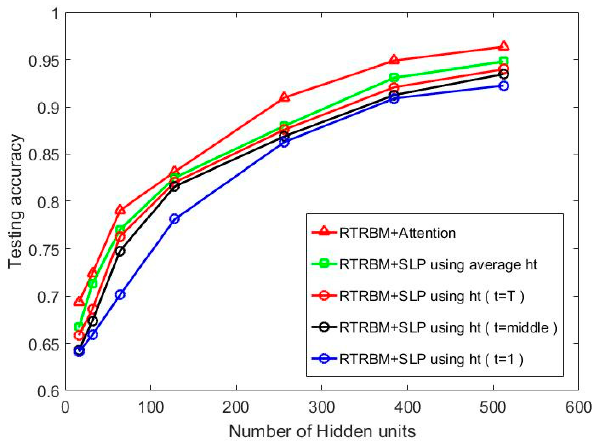
The feature information are extracted by RTRBM and contained in the hidden layer, which are expressed as . We use (the feature of the first, middle, last, and the average of all time frames) as input data, respectively, and classify it with a Single Layer Perceptron (SLP) model. In other words, we can regard the baselines as special forms of ARTRBM that set the coefficients to and respectively. For fair comparison, in this experiment, T is set to 15 and the number of hidden units is 384, which can achieve an ideal accuracy with low computation complexity. Therefore, represents the hidden features when t = 8.
As shown in Figure 9, the proposed model achieves higher recognition accuracy than the other four methods at all hidden layer sizes. This result indicates that the attention mechanism can select discriminatory features more efficiently than other methods that select average or any single . It is worth noting in the figure that choosing average performs better than the other three contrastive experiments. In addition, with the time step t increases, RTRBM+SLP models perform better. This is not surprising since the latter contains more temporal and spatial correlation information through the correlation matrix . However, even the RTRBM+SLP model using still performs worse as our proposed model. Therefore, the attention mechanism greatly contributes to the recognition performance.
5.2.2. Experiment 2: Investigating the Influence of SNR on Recognition Performance
For applications in real scenarios, white Gaussian noise of different Signal-to-Noise (SNR) increasing from −10dB to 30dB were added to the testing data to investigate the robustness of the proposed model. In addition, the test data with different SNR are shown in Figure 10.
As shown in Figure 10, white Gaussian noise of different SNRs is superimposed on the test HRRP sequence. Each row in the figure represents the index of range cell while each column shows the number of testing data. We use T72 as example, which contains 5820 HRRP samples.
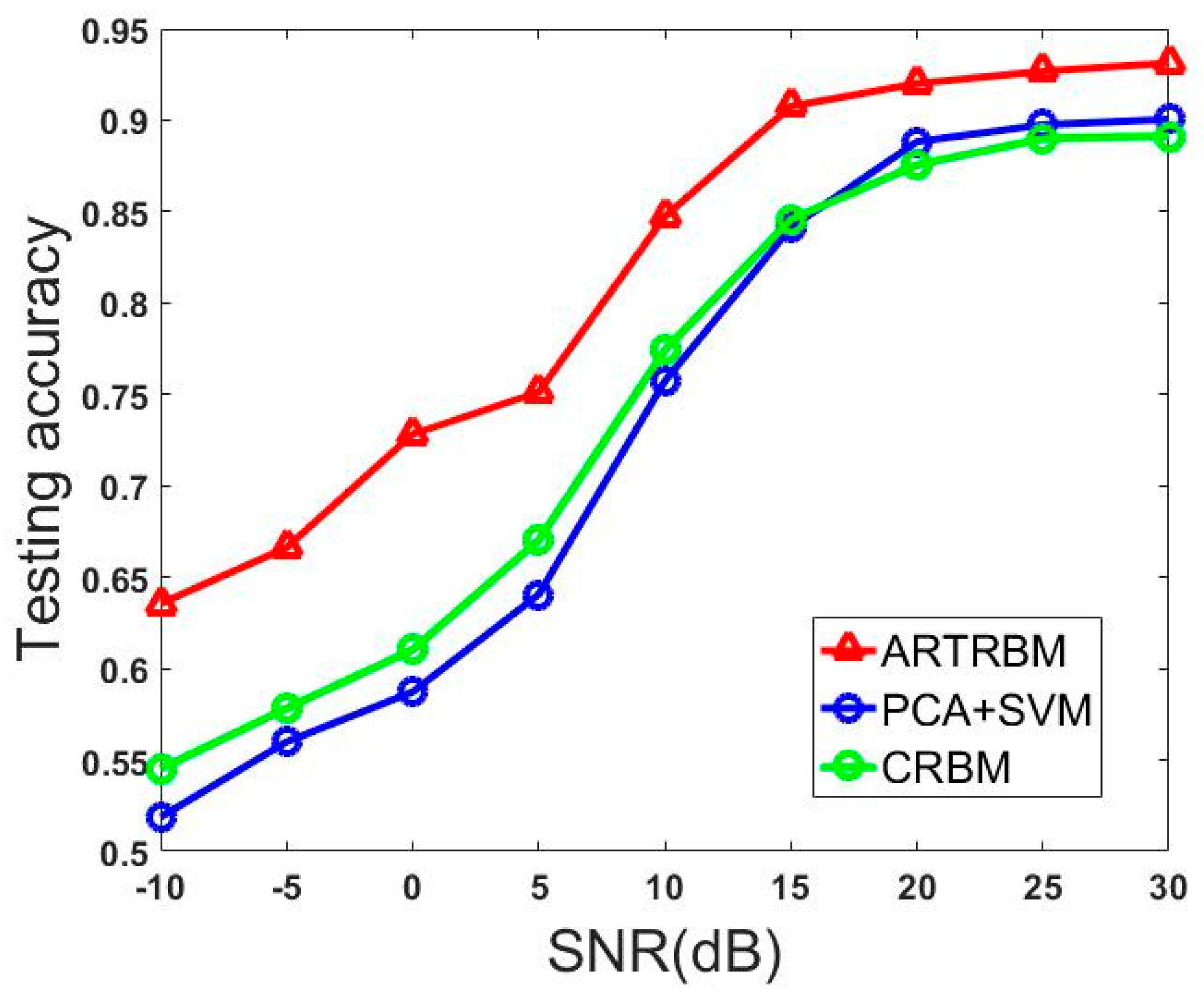
In this example, we trained the ARTRBM using the HRRP sequence with T = 15 and 384 hidden units. We choose the Class RBM with 384 hidden units as the contrast experiment and the data input method connected 15 HRRPs end to end, which performs better than all other contrastive experiments in Experiment 1. Another contrast experiment uses PCA to reduce the dimension to 15 of input data and the classifier is the Support Vector Machine (SVM).
Figure 11 shows the recognition performance of three models with different SNR. It is obvious that our proposed model achieves better performance than the other two models at all SNR levels and it gets more than 10% advantage over the other two models at −10dB. Additionally, the testing accuracy keeps stable at a high level, which is near the average accuracy in Table 2 (0.9488) when the SNR is higher than 15dB, which inflects that our proposed model has a certain anti-noise ability. The accuracy of the proposed model decreases to about 65% with the decrease of SNR. However, this number is less than 55% for CRBM. This result shows the strong anti-noise power of ARTRBM. Considering the working environment of the radar system, the training samples are often corrupted by noise. The model we proposed is a better choice to perform the HRRP sequence recognition task.
6. Conclusions
In this paper, attention-based RTRBM is proposed for target recognition based on the HRRP sequence. Compared with the reported methods, the proposed method has some compelling advantages. First, it introduces the correlation matrix between the hidden layers to extract more correlation information, which makes the extracted features hold the previous and current information. Afterward, it efficiently deals with high dimensional sequential data, which performs better than Class RBM using two different data input methods. Additionally, it can be effective for choosing and utilizing the important parts of the extracted features, which outperforms the RTRBM+SLP model using different input features. Additionally, the proposed model performs well in the case of strong noise, which indicates a strong robustness for the noise. In the near future, to better solve the problem of sequential HRRP recognition, we plan to combine other deeper models with an attention mechanism as a classifier for RTRBM or other sequential feature extraction models. Furthermore, in order to make the model more applicable to the real scenario, we will operate related experiments in the cases of different waveforms and pulse recurrence intervals (PRIs) or the case of the training phase and testing phase at different angular sampling rates. Additionally, we attempt to develop a model that can set the length of the attention mechanism adaptively. In this case, the number of T will not need to be set by experience, which may achieve a better performance.
Author Contributions
X.G. and Y.Z. conceived and designed the experiments. X.P. contributed the MSTAR dataset. Y.Z. performed the experiments. Y.Z. and X.P. analyzed the data. Y.Z. and J.Y. wrote the paper. X.L. supervised this paper.
Funding
This work is funded by the National Science Foundation of China under contract No.61501481 and the National Natural Science Foundation of China under contract No. 61571450.
Conflicts of Interest
The authors declare no conflict of interest.
Appendix A
According to Equation (11), we get:
In order to compute , we need to compute first, which is shown in the equation below.
Therefore, we get:
where
is calculated by Equation (4).
According to Equation (A1) and (A4), we get:
Similarly, the gradients can be represented by the equations below.
and the gradients are represented below.
Appendix B
According to Equation (15) and (17), we get:
where , and .
Similarly, we get:
Submitting Equations (15)–(17) into Equation (14), respectively, the gradients can be computed exactly, which are shown below.
where
References
- Du, L.; Liu, H.; Bao, Z. Radar HRRP statistical recognition: Parametric model and model selection. IEEE Trans. Signal Proc. 2008, 56, 1931–1944. [Google Scholar] [CrossRef]
- Webb, A.R. Gamma mixture models for target recognition. Pattern Recognit. 2000, 33, 2045–2054. [Google Scholar] [CrossRef]
- Du, L.; Wang, P.; Zhang, L.; He, H.; Liu, H. Robust statistical recognition and reconstruction scheme based on hierarchical Bayesian learning of HRR radar target signal. Expert Syst. Appl. 2015, 42, 5860–5873. [Google Scholar] [CrossRef]
- Zhou, D. Orthogonal maximum margin projection subspace for radar target HRRP recognition. Eurasip J. Wirel. Commun. Netw. 2016, 1, 72. [Google Scholar] [CrossRef]
- Zhang, J.; Bai, X. Study of the HRRP feature extraction in radar automatic target recognition. Syst. Eng. Electron. 2007, 29, 2047–2053. [Google Scholar]
- Du, L.; Liu, H.; Bao, Z.; Zhang, J. Radar automatic target recognition using complex high resolution range profiles. IET Radar Sonar Navi. 2007, 1, 18–26. [Google Scholar] [CrossRef]
- Feng, B.; Du, L.; Liu, H.W.; Li, F. Radar HRRP target recognition based on K-SVD algorithm. In Proceedings of the IEEE CIE International Conference on Radar, Chengdu, China, 24–27 October 2011; pp. 642–645. [Google Scholar]
- Huether, B.M.; Gustafson, S.C.; Broussard, R.P. Wavelet preprocessing for high range resolution radar classification. IEEE Trans. 2001, 37, 1321–1332. [Google Scholar] [CrossRef]
- Zhu, F.; Zhang, X.D.; Hu, Y.F. Gabor Filter Approach to Joint Feature Extraction and Target Recognition. IEEE Trans. Aerosp. Electron. Syst. 2009, 45, 17–30. [Google Scholar]
- Hu, P.; Zhou, Z.; Liu, Q.; Li, F. The HMM-based modeling for the energy level prediction in wireless sensor networks. In Proceedings of the IEEE Conference on Industrial Electronics and Applications (ICIEA 2007), Harbin, China, 23–25 May 2007; pp. 2253–2258. [Google Scholar]
- Rossi, S.P.; Ciuonzo, D.; Ekman, T. HMM-based decision fusion in wireless sensor networks with noncoherent multiple access. IEEE Commun. Lett. 2015, 19, 871–874. [Google Scholar] [CrossRef]
- Albrecht, T.W.; Gustafson, S.C. Hidden Markov models for classifying SAR target images. Def. Secur. Int. Soc. Opt. Photonics 2004, 5427, 302–308. [Google Scholar]
- Liao, X.; Runkle, P.; Carin, L. Identification of ground targets from sequential high range resolution radar signatures. IEEE Trans. 2002, 38, 1230–1242. [Google Scholar]
- Zhu, F.; Zhang, X.D.; Hu, Y.F.; Xie, D. Nonstationary hidden Markov models for multiaspect discriminative feature extraction from radar targets. IEEE Trans. Signal Proc. 2007, 55, 2203–2214. [Google Scholar] [CrossRef]
- Elbir, A.M.; Mishra, K.V.; Eldar, Y.C. Cognitive Radar Antenna Selection via Deep Learning. arXiv, 2018; arXiv:1802.09736. [Google Scholar]
- Su, B.; Lu, S. Accurate scene text recognition based on recurrent neural network. In Proceedings of the 12th Asia Conference on Computer Vision, Singapore, 1−5 November 2014; pp. 35–48. [Google Scholar]
- He, K.; Zhang, X.; Ren, S.; Sun, J. Deep Residual Learning for Image Recognition. In Proceedings of the IEEE Conference on Computer Vision and Pattern Recognition, Danvers, MA, USA, 27–30 June 2016; pp. 770–778. [Google Scholar]
- Hinton, G.E. Training products of experts by minimizing contrastive divergence. Neural Comput. 2002, 14, 1771–1800. [Google Scholar] [CrossRef] [PubMed]
- Sutskever, I.; Hinton, G.E.; Taylor, G.W. The Recurrent Temporal Restricted Boltzmann Machine. In Proceedings of the 25th International Conference on Machine Learning (ICML), Helsinki, Finland, 5–9 July 2008; pp. 536–543. [Google Scholar]
- Cherla, S.; Tran, S.N.; Garcez, A.D.A.; Weyde, T. Discriminative Learning and Inference in the Recurrent Temporal RBM for Melody Modelling. In Proceedings of the International Joint Coference on Neural Networks (IJCNN), Killarney, Ireland, 12–17 July 2015; pp. 1–8. [Google Scholar]
- Mittelman, R.; Kuipers, B.; Savarese, S.; Lee, H. Structured Recurrent Temporal Restricted Boltzmann Machines. In Proceedings of the 31st International Conference on Machine Learning, Beijing, China, 21–26 June 2014; pp. 1647–1655. [Google Scholar]
- Sutskever, I.; Hinton, G. Learning Multilevel Distributed Representations for High Dimentional Sequences. In Proceedings of the Eleventh International Conference on Artificial Intelegence and Statistics, Toronto, ON, Canada, 21−24 March 2007; pp. 548–555. [Google Scholar]
- Boulanger-Lewandowski, N.; Bengio, Y.; Vincent, P. Modeling Temporal Dependencies in High-Dimensional Sequences: Application to Polyphonic Music Generation and Transcription. In Proceedings of the 29th International Conference on Machine Learning, Edinburgh, UK, 27 June–3 July 2012. [Google Scholar]
- Martens, J.; Sutskever, I. Learning recurrent neural networks with Hessian-free optimization. In Proceedings of the 28th International Conference on Machine Learning (ICML-11), Bellevue, WA, USA, 28 June–2 July 2011; pp. 1033–1040. [Google Scholar]
- Smolensky, P. Information processing in dynamical systems: Foundations of harmony theory. Parallel Distrib. Exp. Microstruct. Found 1986, 1, 194–281. Available online: http://www.dtic.mil/dtic/tr/fulltext/u2/a620727.pdf (accessed on 5 March 2018).
- Fischer, A.; Igel, C. Training restricted Boltzmann machines: An introduction Pattern Recognition. Pattern Recognit. 2014, 47, 25–39. [Google Scholar] [CrossRef]
- Larochelle, H.; Bengio, Y. Classification using Discriminative Restricted Boltzmann Machines. In Proceedings of the 25th international conference on Machine learning, Helsinki, Finland, 5–9 July 2008; pp. 536–543. [Google Scholar]
- Salakhutdinov, R.; Mnih, A.; Hinton, G. Restricted Boltzmann Machines for collaborative filtering. In Proceedings of the 24th international conference on Machine learning, Corvalis, OR, USA, 20–24 June 2007; pp. 791–798. [Google Scholar]
- Chorowski, J.; Bahdanau, D.; Serdyuk, D.; Cho, K.; Bengio, Y. Attention Based Models for Speech Recognition. In Proceedings of the Advances in Neural Information Processing Systems, Montreal, QC, Canada, 8–13 December 2014. [Google Scholar]
- Mnih, V.; Heess, N.; Graves, A. Recurrent models of visual attention. In Proceedings of the Advances in Neural Information Processing Systems, Montreal, QC, Canada, 8–13 December 2014; pp. 2204–2212. [Google Scholar]
- Bahdanau, D.; Cho, K.; Bengio, Y. Neural Machine Translation by Jiontly to Align and Translate. arXiv, 2014; arXiv:1409.0473. [Google Scholar]
- Luong, M.; Manning, C.D. Effective Approaches to Attention based Machine Translation. arXiv, 2015; arXiv:1508.04025. [Google Scholar]
- Yin, W.; Ebert, S.; Schütze, H. Attention-Based Convolutional Neural Network for Machine Comprehension. arXiv, 2016; arXiv:1602.04341. [Google Scholar]
- Dhingra, B.; Liu, H.; Cohen, W.; Salakhutdinov, R. Gated-Attention Readers for Text Comprehension. arXiv, 2016; arXiv:1606.01549. [Google Scholar]
- Wang, L.; Cao, Z.; De Melo, G.; Liu, Z. Relation Classification via Multi-Level Attention CNNs. In Proceedings of the 54th Annual Meeting of the Association for Computational Linguistics, Berlin, Germany, 7–12 August 2016; pp. 1298–1307. [Google Scholar]
- Zhou, P.; Shi, W.; Tian, J.; Qi, Z.; Li, B.; Hao, H.; Xu, B. Attention-Based Bidirectional Long Short-Term Memory Networks for Relation Classification. In Proceedings of the 54th Annual Meeting of the Association for Computational Linguistics, Berlin, Germany, 7–12 August 2016; Volume 2, pp. 207–212. [Google Scholar]
- MSTAR (Public) Targets: T-72, BMP-2, BTR-70, SLICY. Available online: http://www.mbvlab.wpafb.af.mil/public/MBVDATA (accessed on 2 March 2018).
- Hinton, G.E. A practical guide to training restricted Boltzmann machines. In Neural Networks: Tricks of the Trade, 2nd ed.; Springer: Heidelberg, Germany; Dordrecht, The Netherlands; London, UK; New York, NY, USA, 2012; pp. 599–619. [Google Scholar]
- Hinton, G.E.; Salakhutdinov, R.R. Reducing the Dimensionality of Data with Neural Networks. Science 2006, 313, 504–507. [Google Scholar] [CrossRef] [PubMed]
- Odense, S.; Edwards, R. Universal Approximation Results for the Temporal Restricted Boltzmann Machine and Recurrent Temporal Restricted Boltzmann Machine. J. Mach. Learn. Res. 2016, 17, 1–21. [Google Scholar]
- Tieleman, T. Training restricted Boltzmann machines using approximations to the likelihood gradient. In Proceedings of the 25th international conference on Machine learning, Helsinki, Finland, 5–9 July 2008; pp. 1064–1071. [Google Scholar]
- Ghader, H.; Monz, C. What does Attention in Neural Machine Translation Pay Attention to. Available online: https://arxiv.org/pdf/1710.03348 (accessed on 7 March 2018).
- Zhao, F.; Liu, Y.; Huo, K.; Zhang, S.; Zhang, Z. Rarar HRRP Target Recognition Based on Stacked Autoencoder and Extreme Learning Machine. Sensors 2018, 18, 173. [Google Scholar] [CrossRef] [PubMed]
- Peng, X.; Gao, X.; Zhang, Y.; Li, X. An Adaptive Feature Learning Model for Sequential Radar High Resolution Range Profile Recognition. Sensors 2017, 17, 1675. [Google Scholar] [CrossRef] [PubMed]
- Vaawani, A.; Shazeer, N.; Parmar, N. Attention is all you need. In Proceedings of the 31st Annual Conference on Neural Information Processing Systems (NIPS), Long Beach, CA, USA, 4–9 December 2017; pp. 6000–6010. [Google Scholar]
Figure 1.
Graphical depiction of the RBM.

Figure 2.
Graphical structure of the RTRBM.

Figure 3.
Graphical structure of Attention-based RTRBM.

Figure 4.
The process of Attention-based RTRBM.
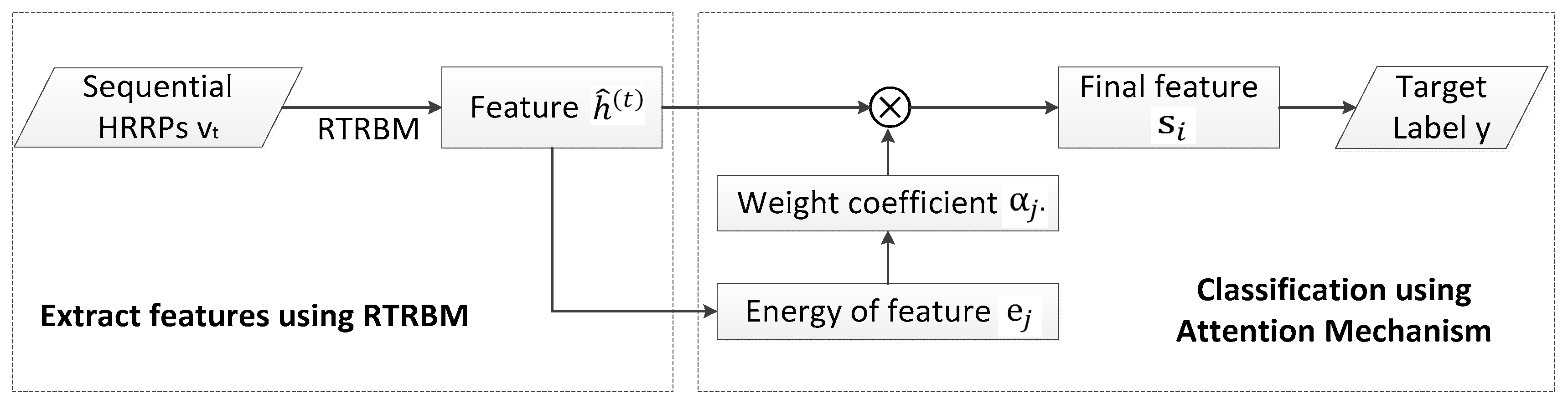
Figure 5.
HRRPs of the three targets. (a) BMP2(Sn_C9563), (b) T72(Sn-132), (c) BTR70(Sn_71).
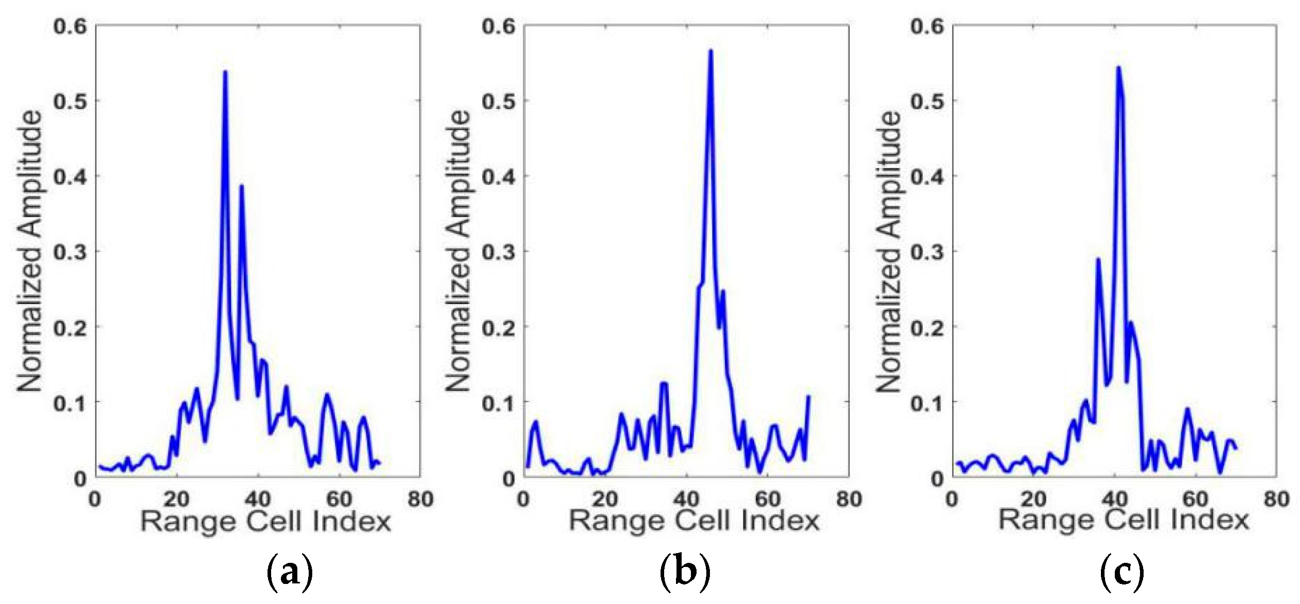
Figure 6.
The composition of the sequential HRRP datasets.
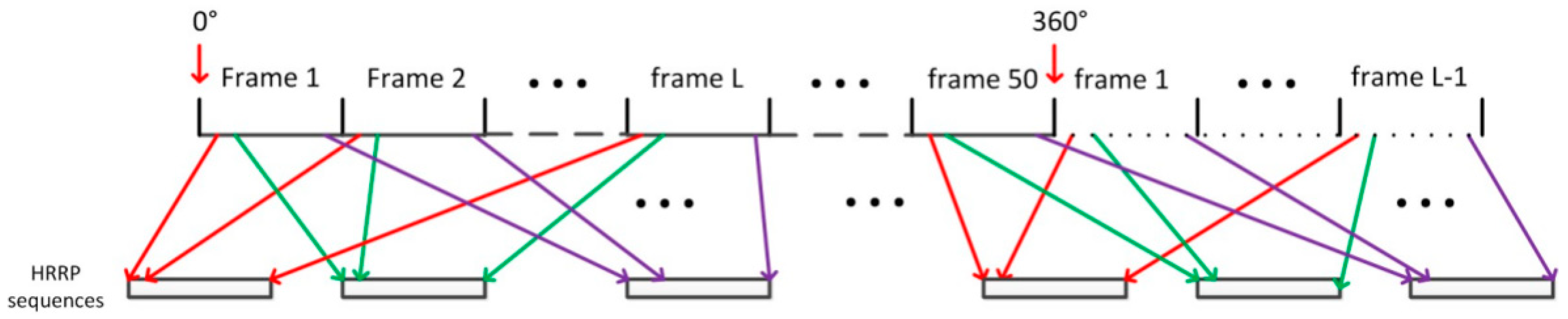
Figure 7.
The recognition performance on five models with a different number of hidden units at T = 15.
Figure 7.
The recognition performance on five models with a different number of hidden units at T = 15.

Figure 8.
Range profiles of three types of BMP2. (a) Sn_C9563, (b) Sn_C9566, (c) Sn_C21.

Figure 9.
Recognition performance on models trained with features extracted by RTRBM.

Figure 10.
Testing HRRP data with different SNR (a) SNR = 20 dB, (b) SNR = 10 dB, (c) SNR = 5 dB.
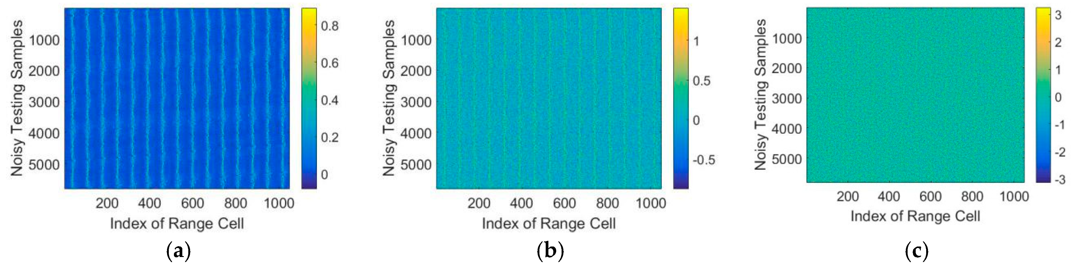
Figure 11.
Recognition performance on models tested with different SNR.


Table 1.
Training and testing set of HRRPs for three targets.
| Number | Training Set | Size | Testing Set | Size |
|---|---|---|---|---|
| 1 | BMP2 (Sn_C9563) | 2330 | BMP2 (Sn_C9563) | 1950 |
| BMP2 (Sn_C9566) | 1960 | |||
| BMP2 (Sn_C21) | 1960 | |||
| 2 | T72 (Sn_132) | 2320 | T72 (Sn_132) | 1960 |
| T72 (Sn_812) | 1950 | |||
| T72 (Sn_S7) | 1910 | |||
| 3 | BTR70 (Sn_C71) | 2330 | BTR70 (Sn_C71) | 1960 |
| Sum | Training Set | 6980 | Testing Set | 13650 |
Table 2.
The accuracy of different lengths of RTRBM.
| Length of RTRBM | T = 5 | T = 10 | T = 15 | T = 20 | T = 25 | T = 30 |
|---|---|---|---|---|---|---|
| Hidden Units | 128 | 128 | 128 | 128 | 128 | 128 |
| BMP2 | 0.5496 | 0.5556 | 0.6649 | 0.6856 | 0.6900 | 0.6915 |
| T72 | 0.7472 | 0.8345 | 0.8575 | 0.8545 | 0.8723 | 0.8789 |
| BTR70 | 0.7594 | 0.8803 | 0.9368 | 0.9402 | 0.9402 | 0.9428 |
| Average Accuracy | 0.6854 | 0.7535 | 0.8197 | 0.8268 | 0.8341 | 0.8377 |
Table 3.
Confusion matrix of the model with 384 hidden units.
| Methods | Attention Based RTRBM | CRBM (Connected HRRPs) | CRBM (Average HRRP) | ||||||
|---|---|---|---|---|---|---|---|---|---|
| Targets | BMP2 | T72 | BTR70 | BMP2 | T72 | BTR70 | BMP2 | T72 | BTR70 |
| BMP2 | 0.9053 | 0.0717 | 0.0230 | 0.8461 | 0.0821 | 0.0718 | 0.8547 | 0.0819 | 0.0634 |
| T72 | 0.0125 | 0.9758 | 0.0117 | 0.0187 | 0.9726 | 0.0087 | 0.0295 | 0.9516 | 0.0189 |
| BTR70 | 0.0347 | 0 | 0.9653 | 0.0448 | 0.0052 | 0.9500 | 0.0525 | 0.0094 | 0.9381 |
| Av. Acc. | 0.9448 | 0.9229 | 0.9157 | ||||||
© 2018 by the authors. Licensee MDPI, Basel, Switzerland. This article is an open access article distributed under the terms and conditions of the Creative Commons Attribution (CC BY) license (http://creativecommons.org/licenses/by/4.0/).
Share and Cite
MDPI and ACS Style
Zhang, Y.; Gao, X.; Peng, X.; Ye, J.; Li, X. Attention-Based Recurrent Temporal Restricted Boltzmann Machine for Radar High Resolution Range Profile Sequence Recognition. Sensors 2018, 18, 1585. https://doi.org/10.3390/s18051585
AMA Style
Zhang Y, Gao X, Peng X, Ye J, Li X. Attention-Based Recurrent Temporal Restricted Boltzmann Machine for Radar High Resolution Range Profile Sequence Recognition. Sensors. 2018; 18(5):1585. https://doi.org/10.3390/s18051585
Chicago/Turabian StyleZhang, Yifan, Xunzhang Gao, Xuan Peng, Jiaqi Ye, and Xiang Li. 2018. "Attention-Based Recurrent Temporal Restricted Boltzmann Machine for Radar High Resolution Range Profile Sequence Recognition" Sensors 18, no. 5: 1585. https://doi.org/10.3390/s18051585
Note that from the first issue of 2016, this journal uses article numbers instead of page numbers. See further details here.