On-Line Temperature Estimation for Noisy Thermal Sensors Using a Smoothing Filter-Based Kalman Predictor


School of Electronics and Information, Northwestern Polytechnical University, Xi’an 710072, China
*
Author to whom correspondence should be addressed.
Sensors 2018, 18(2), 433; https://doi.org/10.3390/s18020433
Submission received: 16 November 2017
/
Revised: 15 January 2018
/
Accepted: 26 January 2018
/
Published: 2 February 2018
(This article belongs to the Special Issue Advances in Infrared Imaging: Sensing, Exploitation and Applications)
Abstract
:Dynamic thermal management (DTM) mechanisms utilize embedded thermal sensors to collect fine-grained temperature information for monitoring the real-time thermal behavior of multi-core processors. However, embedded thermal sensors are very susceptible to a variety of sources of noise, including environmental uncertainty and process variation. This causes the discrepancies between actual temperatures and those observed by on-chip thermal sensors, which seriously affect the efficiency of DTM. In this paper, a smoothing filter-based Kalman prediction technique is proposed to accurately estimate the temperatures from noisy sensor readings. For the multi-sensor estimation scenario, the spatial correlations among different sensor locations are exploited. On this basis, a multi-sensor synergistic calibration algorithm (known as MSSCA) is proposed to improve the simultaneous prediction accuracy of multiple sensors. Moreover, an infrared imaging-based temperature measurement technique is also proposed to capture the thermal traces of an advanced micro devices (AMD) quad-core processor in real time. The acquired real temperature data are used to evaluate our prediction performance. Simulation shows that the proposed synergistic calibration scheme can reduce the root-mean-square error (RMSE) by 1.2 C and increase the signal-to-noise ratio (SNR) by 15.8 dB (with a very small average runtime overhead) compared with assuming the thermal sensor readings to be ideal. Additionally, the average false alarm rate (FAR) of the corrected sensor temperature readings can be reduced by 28.6%. These results clearly demonstrate that if our approach is used to perform temperature estimation, the response mechanisms of DTM can be triggered to adjust the voltages, frequencies, and cooling fan speeds at more appropriate times.
1. Introduction
The field of integrated circuit technology is entering the nanometer era. However, excessively increased power density leads to high chip temperature, which can result in thermal runaway. Elevated die temperature adversely affects the performance of multi-core processor systems, causing shortened lifetimes, increased cooling costs, and reduced reliability and device speed [1]. Therefore, reliable and effective thermal monitoring mechanisms are crucial to overcome this challenge. Dynamic thermal management (DTM) is often employed to continuously track the thermal behavior of processors during runtime [2]. Typically, on-die thermal sensors are widely deployed in modern multi-core processors to assist DTM [3]. According to the fine-grained temperature information collected by embedded thermal sensors, DTM techniques maintain the processor’s temperature within a preset range by reasonably assigning workload scheduling, and adjusting the voltages, frequencies, and cooling fan speeds appropriately [4,5]. In addition, in order to mitigate thermal emergencies on multi-core chips, only a fraction of cores can be simultaneously powered in the full performance mode, while other cores (i.e., dark cores) need to be power gated. In this so-called dark silicon problem [6,7,8,9] is important to ensure thermal-safe operation for modern chips, i.e., where the peak temperature does not exceed the safe-operating temperature, otherwise the response mechanisms of DTM are triggered.
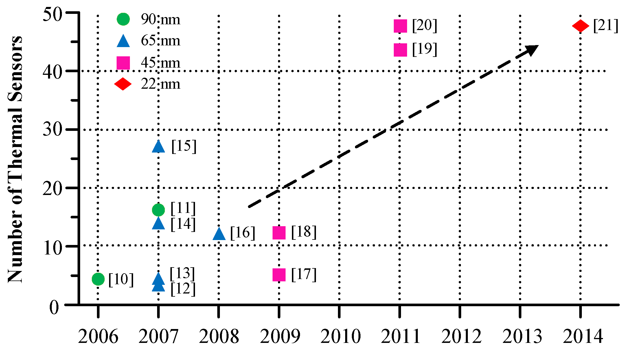
The number of on-die thermal sensors keeps growing in very large scale integration (VLSI) systems to enable the DTM of chip functionalities [10,11,12,13,14,15,16,17,18,19,20,21], as shown in Figure 1. The accuracy of on-chip sensor readings has a great influence on the effectiveness and reliability of DTM. However, embedded thermal sensors are inevitably accompanied by noise, including process variation, supply voltage fluctuations, and cross-coupling etc, which cause the observed temperature readings to deviate from the actual values. In the worst case, the temperature reading error of un-calibrated thermal sensors used in IBM25PPC750L processors (International Business Machines Corporation (IBM), Armonk, New York, United States of America) can be up to 34 C (at an actual temperature of 95 C) [22]. Therefore, blindly trusting the thermal sensors to be ideal can lead DTM strategies to make inaccurate decisions that result in false alarms or unnecessary responses.
Thermal monitoring and management in VLSI systems have been widely researched in recent years [23,24,25]. Nowroz et al. [26] utilized frequency-domain signal representations to devise both static and runtime thermal monitoring approaches. Unfortunately, this work does not consider the effect of inaccurate and noisy sensors. Reda et al. [27] proposed a new direction to simultaneously identify the thermal models and the fine-grain power consumption of a chip from just the measurements of the thermal sensors and the total power consumption. Although they verified the accuracy of this method and demonstrated its resilience to sensor noise, the problem of noise reduction for sensor measurements was not addressed. Effective temperature calibration can compensate for inaccuracies in temperature measurement, and help to improve thermal sensing accuracy. As a result, how to solve the problem of estimating temperatures for on-chip thermal sensors corrupted by noise is a major challenge.
A number of studies have taken into account the noise issue associated with sensor readings, such as the statistical methodology [28] and the multi-sensor collaborative calibration algorithm (MSCCA) [29]. However, these techniques lack the ability for real-time prediction which is required for proactive DTM techniques [30]. In [31,32], the authors proposed a scheme to make online temperature measurements significantly more accurate. They constructed an offline thermal equivalent resistor–capacitor (RC) model and reduced its complexity by a projection-based model order reduction method. This model can be used to convert the power dissipation to temperature in the prediction step of the Kalman filter. However, the derivation of such an RC model is not trivial due to the complexity of silicon materials. Unlike the above approach, we apply the polynomial fitting technique to convert the oscillation frequency of noisy sensors to temperature data and use the smoothing filter to obtain the prediction information. These two sources of temperature information are then combined in the Kalman filter to generate reliable temperature estimations. This direct method reduces the calibration cost because it eliminates the requirement for estimating the power consumption per functional unit. Specifically, the contributions of this work are as follows:
- The noise characteristics of on-chip thermal sensors based on the ring oscillator structure are systematically analyzed. On this basis, the polynomial fitting technique is used to establish the non-linear relationship between sensor temperature and oscillation frequency, which can improve the measurement accuracy.
- To tackle the challenge in temperature estimation of noisy thermal sensors, a smoothing filter-based Kalman prediction technique is proposed to correct the temperatures of on-die sensors in real-time.
- For the multi-sensor estimation scenario, the spatial correlations among different sensor locations are exploited. On this basis, a multi-sensor synergistic calibration algorithm (called MSSCA) is proposed to improve the simultaneous prediction accuracy of multiple sensors.
- Relative to the previous works relied on computer-based thermal simulation scheme, an infrared imaging-based temperature measurement technique is proposed to provide the accurate thermal characterizations of an AMD quad-core processor operating on different benchmarks. The captured real temperature data are used to evaluate our prediction approach.
The remainder of this paper is organized as follows: Section 2 provides the necessary motivation of this work, and presents the analysis of noisy sensor behavior. Section 3 presents the on-line temperature estimation technique using a smoothing filter-based Kalman predictor, and details the proposed multi-sensor synergistic calibration algorithm (MSSCA) that can improve the simultaneous prediction accuracy of multiple sensors. Section 4 describes the infrared temperature measurement setup required for capturing the thermal traces of real processors. The performance of our synergistic calibration scheme is validated in Section 5. Finally, we summarize the main conclusions of this work in Section 6.
2. Analysis of Noisy Sensor Behavior
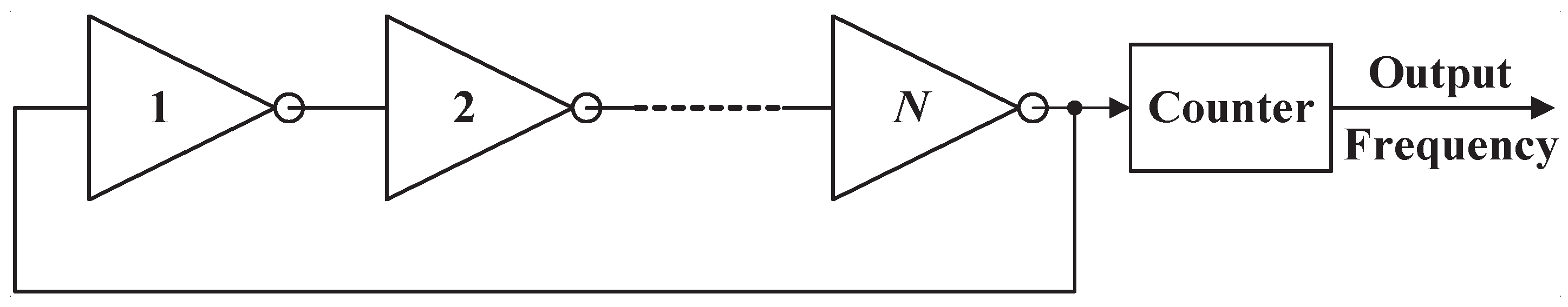
Due to the unpredictable behavior of the chip’s thermal profile, constantly monitoring the processor’s temperature using embedded thermal sensors is critical to ensuring long-term reliability of integrated circuit systems. A classical implementation of on-die thermal sensors is the ring oscillator, which has been known for nearly 30 years [33]. The structure of a typical ring oscillator mainly contains N (an odd number) stages of inverters and a counter, as depicted in Figure 2. Note that the output frequency of ring oscillator in Figure 2 represents the oscillation frequency.
The output frequency depends on the total time-delay of inverters, which is given by the following equation:
where denotes the time-delay with a single inverter switching from the high (low) voltage to the low (high) voltage. The expression for can be described as:
where C and are the effective load capacitance and the oxide capacitance per unit gate area, and are the supply voltage and the threshold voltage, and and are the width/length ratio and the electron mobility of n-metal-oxide-semiconductor (NMOS), respectively. Note that the expression for is identical to Equation (2) except that and need to be replaced with the corresponding parameters of p-metal-oxide-semiconductor (PMOS), i.e., and , respectively. According to Equations (1) and (2), the output frequency is easily affected by temperature since both and are sensitive to temperature. To describe the temperature effects more accurately, the following empirical equations can be used [34]:
where is the reference temperature. As we can see from Equations (3) and (4), drops by 2 mV when temperature increases by 1 C, and also decreases with a more complex relationship when temperature rises. Because dominates in the influence of time-delay, the overall effect appears a decrease of output frequency with temperature rise. Therefore, the output frequency observations can be used to measure the chip temperature.
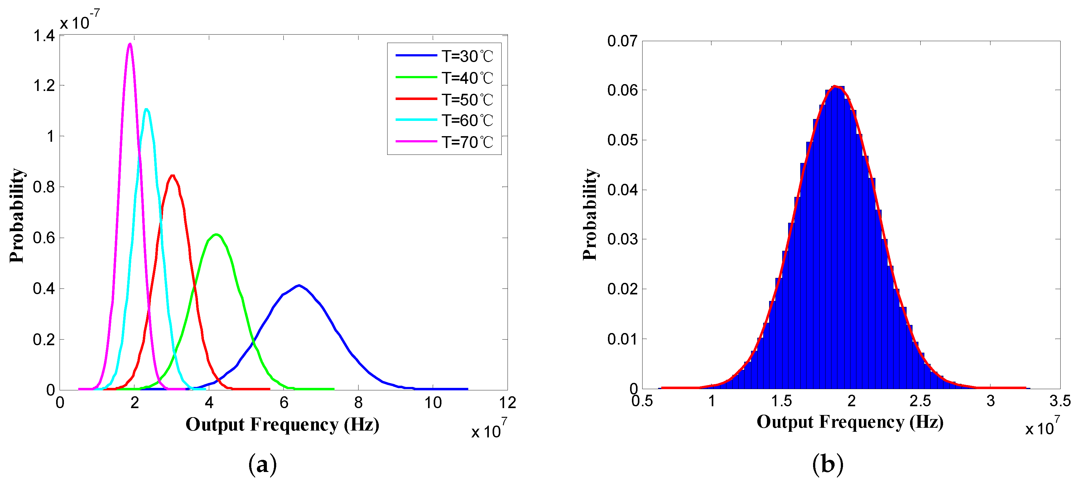
However, due to environmental uncertainty and process variation, the accuracy of output frequency is highly susceptible to several factors, such as variations in process parameters and fluctuations in supply voltage and ambient temperature. Generally, these noise sources can be divided into two main categories, i.e., dynamic noise and static noise. Dynamic noise represents the variation in the accuracy of specific sensors over time, which is caused by fluctuations in supply voltage and ambient temperature. Static noise means variations in the circuit parameters, including load capacitance, oxide capacitance, length/width ratio, etc. To describe the statistical characteristics of output frequency observations under the influence of noise, the following Monte Carlo (MC) simulation is performed using Equations (1)–(4) with 100,000 samples for each different temperature, ranging from 30 C to 70 C with an increment of 10 C. All the random variables are assumed to be the normal distribution with mean values and standard deviations specified in Table 1.
The results of the MC simulation are given in Figure 3. Specifically, the probability density distribution of output frequencies under different temperatures is depicted in Figure 3a. Each curve in Figure 3a shows the potential distribution of output frequencies for a fixed sensor temperature. The integral of the probability density under each curve over the entire space is equal to one. From Figure 3a, it can be observed that these probability density distribution curves heavily overlap with each other, i.e., the same output frequency could be caused by multiple potential temperatures. Therefore, blindly trusting the thermal sensors to be ideal could lead to significant error. This clearly indicates that effective temperature estimation methods are very important for predicting the accurate temperatures from noisy sensor readings. Besides, the statistical histogram of output frequency distribution at the temperature of 70 C is shown in Figure 3b. The statistical histogram divides the entire range of values into a series of intervals, and then counts how many values fall into each interval. In Figure 3b, we divide the entire range of frequencies for the pink curve into 60 intervals on average. The height of each rectangle in Figure 3b indicates the sum of probabilities which fall into the corresponding interval.
3. Temperature Estimation for Noisy Thermal Sensors
Based on the above analysis of noisy sensor behavior, an accurate on-line temperature estimation technique is proposed in this section, which can be divided into the following five steps. The flowchart of our proposed scheme is given in Figure 4.
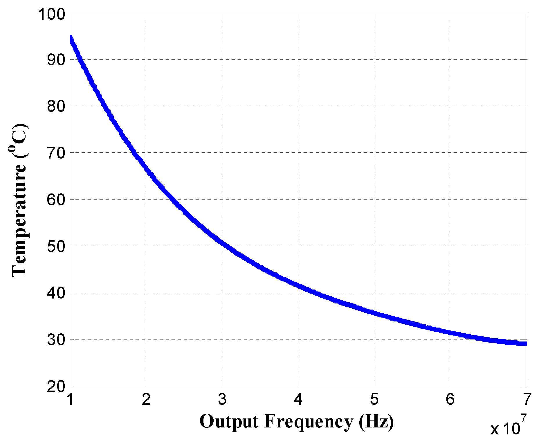
- Step 1: Establish the non-linear relationship between sensor temperature and output frequency using the polynomial fitting technique, and then calculate the temperature observation values of noisy sensors.Based on Equations (1)–(4), we use the mean values of random variables specified in Table 1 to generate the observed data of output frequencies by varying the sensor temperature. The reference temperature is set to 25 C. The actual temperature data is acquired by our infrared temperature measurement setup (described later in Section 4). Using the observed data, the non-linear relationship between sensor temperature and output frequency can be established by the polynomial fitting. The fitting result is shown in Figure 5.
- Step 2: Establish the temperature prediction model using the smoothing filter, and calculate the temperature prediction values of noisy sensors.
- Step 3: Correct the temperatures of noisy sensors using the Kalman filter.
- Step 4: Establish the spatial correlation model, and update the temperature observation values using the multi-sensor synergistic calibration algorithm (MSSCA).
- Step 5: Reuse the Kalman filter to calculate the optimal multi-sensor temperature estimations.
3.1. Smoothing Filter-Based Kalman Prediction Technique
The Kalman filter [35], also known as linear quadratic estimation, is an efficient recursive filter that estimates the internal state of a linear dynamic system from a series of noisy measurements and is popular for its simple implementation and computational complexity. It has been widely used in numerous engineering applications. Recently, the methods based on the Kalman filter have shown the ability to track the temperature profile of a chip in real time. In order to apply the Kalman filter algorithm to predict the temperatures from noisy sensor observations, it is essential to introduce the state space model which is governed by the linear difference Equation (5). Considering the effect of noise and inaccuracy, the observation model is described as Equation (6).
Here, at time instant k, is the state vector representing the predictions, is the measurement vector representing the sensor readings, and and are the process noise vector and the measurement noise vector, respectively. The coefficient matrices and denote the state matrix and the output matrix, respectively.
According to Equations (5) and (6), the Kalman filter algorithm can be employed to estimate the process in a recursive manner, which consists of two distinct phases, namely predict and update. Using the state estimate from the previous time step, the predict phase can generate a priori temperature estimate and error covariance at the current time step. Recently, smoothing filters [36] have attracted significant attention since they work well for many denoising problems. One of the most common smoothing algorithms is the moving average (MA), which is often used to attempt to capture important trends in the observed data. Based on the characteristic that the chip temperature does not suddenly change within short temporal sampling interval, smoothing filters can be used to minimize the impacts of temperature fluctuations. Therefore, a simple moving average (SMA) shown in Equation (7) is designed to achieve a more accurate temperature prediction model. Consequently, the equations of predict phase can be updated as:
where represents the length of the smoothing window, is the covariance matrix of the process noise, is the priori state estimate vector, and , and denote the priori and posteriori error covariance matrix, respectively. The first prediction value is obtained by taking the average of initial temperature estimations in the smoothing window, and then the prediction value is dynamically modified by shifting the window forward. In our case, initial temperature estimations are set to noisy sensor readings. The effects of initial temperature estimations on the smoothing filter are less obvious. However, the length of the smoothing window will directly affect the prediction performance. We have experimentally determined that SMA works best when the length of the smoothing window is equal to 5.
In the update phase, the current priori prediction is combined with the current observation information to obtain an improved posteriori state estimate. The equations of update phase can be expressed as:
where represents the Kalman gain matrix, and denotes the covariance matrix of measurement noise. The framework of the Kalman filter algorithm is illustrated in Figure 6.
3.2. Multi-Sensor Synergistic Calibration Algorithm (MSSCA)
Current VLSI chips deploy multiple sensors to continuously monitor the thermal state of different overheating positions. One important observation is that temperature variations at different sensor locations on the chip are correlated. Typically, sensors close to each other physically are likely to have stronger spatial correlation than sensors far apart [30,37]. Such correlations are caused by similar power behaviors. This phenomenon can be observed by our infrared temperature measurement setup (described later in Section 4). To illustrate the spatial correlation of temperature variations, the temperatures of three different sensor locations are captured, as shown in Figure 7. In particular, the distribution of sensor locations is given in Figure 7a, and the corresponding temperature variations are shown in Figure 7b. The thermal traces confirm that nearby sensors have similar characteristics compared with sensors far apart. Moreover, the variability in process parameters (such as channel width, length, and oxide thickness) can also be correlated, which results in the correlated noisy behavior of sensors. Such correlation models can be established by the statistical static timing analysis (SSTA). In our methodology, the correlation information of fabrication randomness at different sensor locations is considered as well. As compared with treating each sensor independently, the spatial correlation can be used to correct the sensor observations so as to further improve the accuracy of temperature estimation. Therefore, exploiting the spatial correlation is necessary.
There are some studies aimed at the modeling of the spatial correlation [38,39,40]. In [40], the authors applied mathematical theories from random fields and convex analysis to develop robust techniques to extract a valid spatial correlation function from measurement data, and they have experimentally confirmed that the resulting correlation function is the closest ones to the underlying model even if the data are affected by unavoidable random noise. Therefore, the spatial correlation function proposed in [40] is adopted in our methodology. The spatial correlation coefficient () between any two different sensor positions can be described as:
where represents the modified Bessel function of the second kind of order , is the gamma function, and denotes the Euclidean distance between two sensor locations on the chip which is expressed as follows:
where and denote the coordinates of any two sensors. The shape of the spatial correlation function is regulated by the two real parameters b and s. To facilitate for our spatial correlation modeling, a rich set of correlation functions can be obtained by varying b and s, as shown in Figure 8. In our case, b and s are set to 1 and 8, respectively.
Based on the aforementioned spatial correlation model, the multi-sensor synergistic calibration algorithm (MSSCA) is devised to correct the sensor measurements using the correlations. The goal of the MSSCA is to further improve the simultaneous prediction accuracy of multiple sensors. For one arbitrary sensor (denoted as m) of all the M sensors in the monitored region, the MSSCA can be presented in four steps as follows:
- Compute the correlation coefficients (, for and ) of sensor m with all the other sensors, and pick out the largest one (), i.e., sensor m has the strongest correlation with sensor n.
- Set the correlation threshold . If , the temperature measurement of sensor m will not be updated, i.e., ; otherwise, the temperature observation of sensor m can be corrected as:
- Perform steps 1–2 in the residual sensors until the temperature observation of each sensor has been completed in the calibration, and then update the corresponding measurement vector to .
- Calculate the optimal temperature predictions using the following equation:
The pseudo code of the MSSCA is shown in Algorithm 1. Note that the correlation coefficients among all the available sensors comprise the coefficient matrix () of dimension , and is a symmetric matrix in which the elements on the diagonal are all equal to one, as shown in Equation (16).
| Algorithm 1 Multi-Sensor Synergistic Calibration Algorithm (MSSCA) | |
| 1. | Initialize: |
| 2. | Compute the coefficient matrix according to Equation (12) |
| 3. | Remove the autocorrelation by , and store in memory |
| 4. | maxc, and maxl |
| 5. | for to M do |
| 6. | for to M do |
| 7. | if then |
| 8. | , and |
| 9. | end if |
| 10. | end for |
| 11. | end for |
| 12. | for to K do |
| 13. | |
| 14. | for to do |
| 15. | |
| 16. | end for |
| 17. | |
| 18. | |
| 19. | |
| 20. | |
| 21. | |
| 22. | for to M do |
| 23. | if then |
| 24. | else if then |
| 25. | |
| 26. | else if then |
| 27. | |
| 28. | else |
| 29. | end if |
| 30. | end for |
| 31. | |
| 32. | end for |
To remove the autocorrelation, the coefficient matrix can be built as , where denotes the identity matrix. Considering the correlation coefficient only depends on the distance that is not changed because the placement of sensors was fixed at design time, the correlation coefficients only need to be calculated when the MSSCA is first implemented, and then the upper triangular matrix of is stored in memory.
4. Infrared Imaging-Based Temperature Measurement Technique
The inputs to our temperature estimation technique are the thermal traces at a set of discrete sensor positions. These inputs could be generated from either a computer-based thermal simulator or an infrared imaging-based thermal measurement infrastructure. The previous related studies on thermal tracking mainly rely on computer-based simulations. To obtain the thermal traces, these simulations utilize the workload power traces from an architectural-level simulator (e.g., Wattch [41]) together with the floor-plan of processor as inputs to a temperature simulator (e.g., Hotspot [42]). In this section, an infrared imaging-based temperature measurement setup is developed to obtain the accurate thermal characterizations of an AMD quad-core processor operating on different benchmark workloads. Recent studies on thermal measuring have confirmed the value of the complementary information that infrared thermography provided [43,44,45].
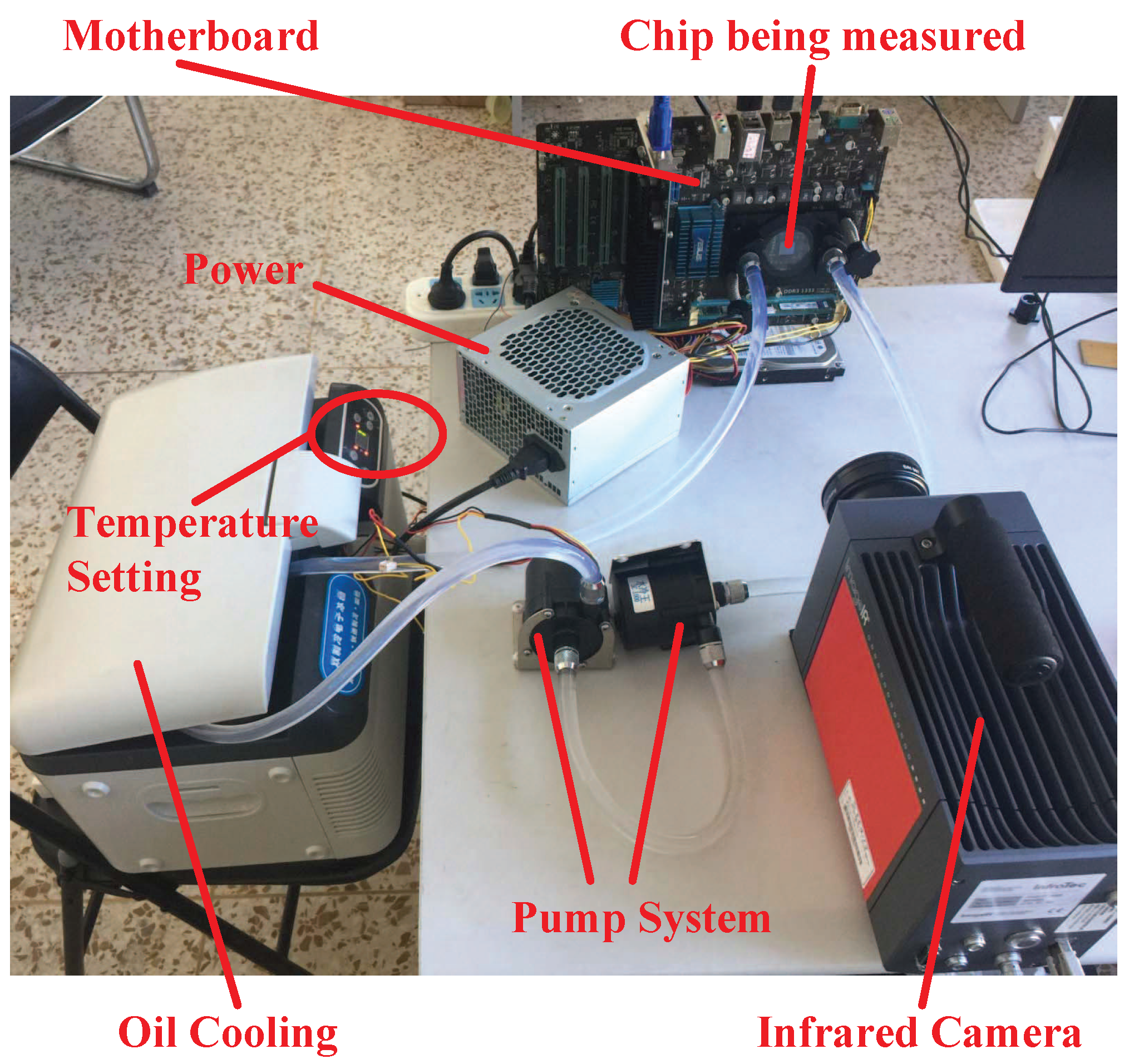
To track the thermal behavior of processor in real-time, an oil-based cooling system is designed to replace the infrared opaque metal heat sink. Once the original metal heat sink is removed, we need an infrared transparent heat sink to dissipate the generated heat adequately. To keep the chip working within a safe temperature range, a distinctive heat sink is devised that contains two layered sapphire windows (with an around 4-mm thickness for each). The proposed infrared temperature measuring equipment is depicted in Figure 9. As compensation for the conventional thermal interface material (TIM), the sapphire window on the top of the die is used to improve lateral heat spreading and increase the thermal capacitance. Due to the relatively high thermal conductivity, large specific heat capacity, and good transparency in the infrared range, mineral oil is a suitable choice for a coolant [44,45]. The mineral oil (Sigma M3156 (Sigma-Aldrich Corporation, St. Louis, Missouri, United States of America)) is persistently pushed through the inlet by an external direct current (DC) pump that circulates between the two layers of sapphire window to transfer the heat. In order to keep the flow laminar, the clearance of two sapphire windows is restricted to 1 mm. The oil temperature is monitored using a thermostat. The detailed thermal traces of the SPEC CPU 2006 (Standard Performance Evaluation Corporation (SPEC), Gainesville, Virginia, United States of America) benchmark workloads [46] are captured using a mid-wave infrared camera (InfraTec ImageIR® 8300 (InfraTec GmbH Infrarotsensorik und Messtechnik, Dresden, Germany)). Because the lightly doped and undoped silicon are partially transparent at the mid-wave infrared range, the chip temperature can be measured through our tailored infrared transparent heat sink. The chip being tested is a 45-nm AMD Athlon II X4 610e (Advanced Micro Devices, Inc. (AMD), Santa Clara, California, United States of America) quad-core processor [47] operating at 2.4 GHz. The image of our experimental setup is exhibited in Figure 10. To demonstrate the effectiveness of our infrared thermography technique, a few examples of thermal traces are shown in Figure 11.
5. Experimental Results
In this section, the performance of our temperature estimation approach is verified using the real thermal traces obtained by the above infrared temperature measurement setup. In what follows, we consider the case that three thermal sensors (denoted as P1, P2, and P3) are placed on the chip (see Figure 7a), and we try to calibrate their temperatures from the noisy sensor observations. It should be noted that the approach is the same for more than three sensors. The correlation coefficients among all three sensors are calculated according to Equation (12) as shown in Table 2, and the correlation threshold () is set to 0.8. The random parameters of thermal sensors are assumed to be of normal distribution, and we set the mean values of these parameters to be the standard values used in the 180-nm fabrication process (see Table 1). The dynamic noise source is assumed to have a supply voltage () fluctuation. Then, the MC simulation is performed based on Equations (1)–(4) to generate the noisy sensor readings that are used to test our temperature estimation. All the simulations are implemented by MATLAB code running on an Intel Core (Intel Corporation, Santa Clara, California, United States of America) 3.2 GHz computer with 16 GB synchronous dynamic random access memory (SDRAM).
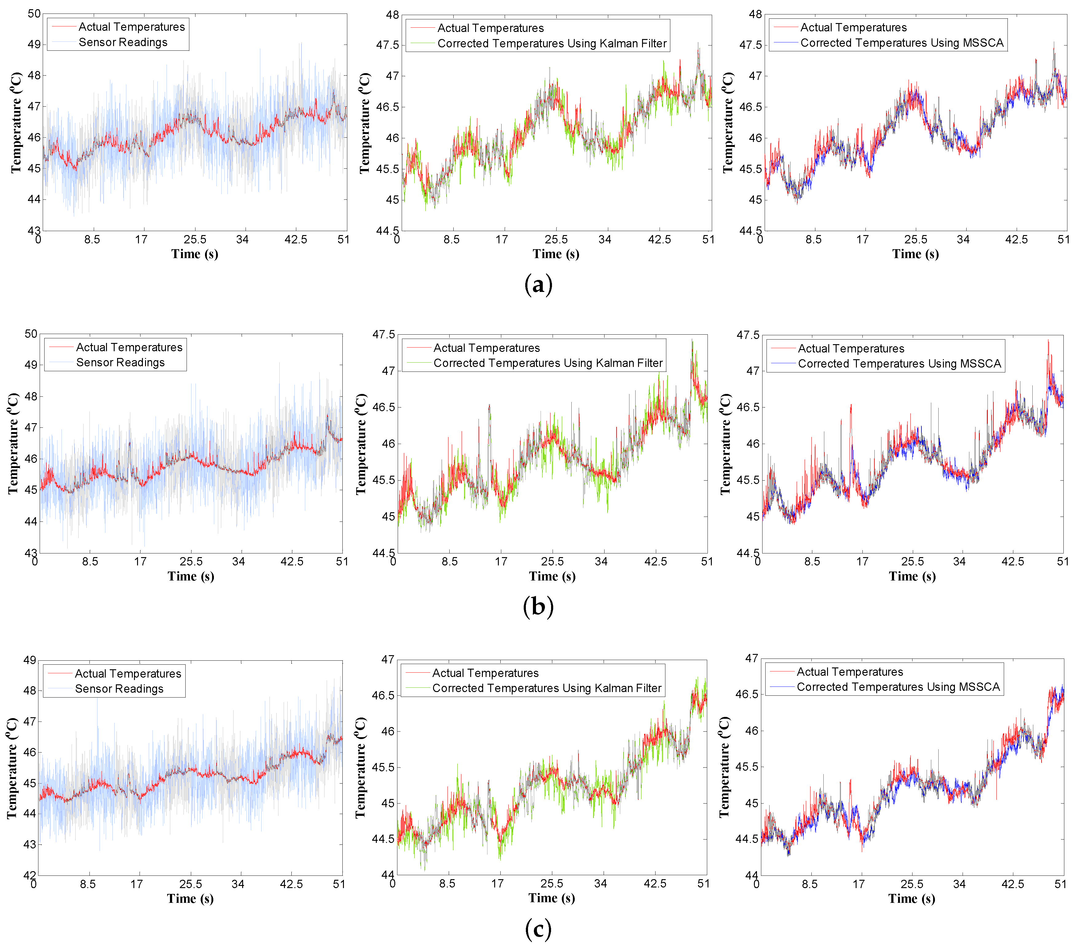
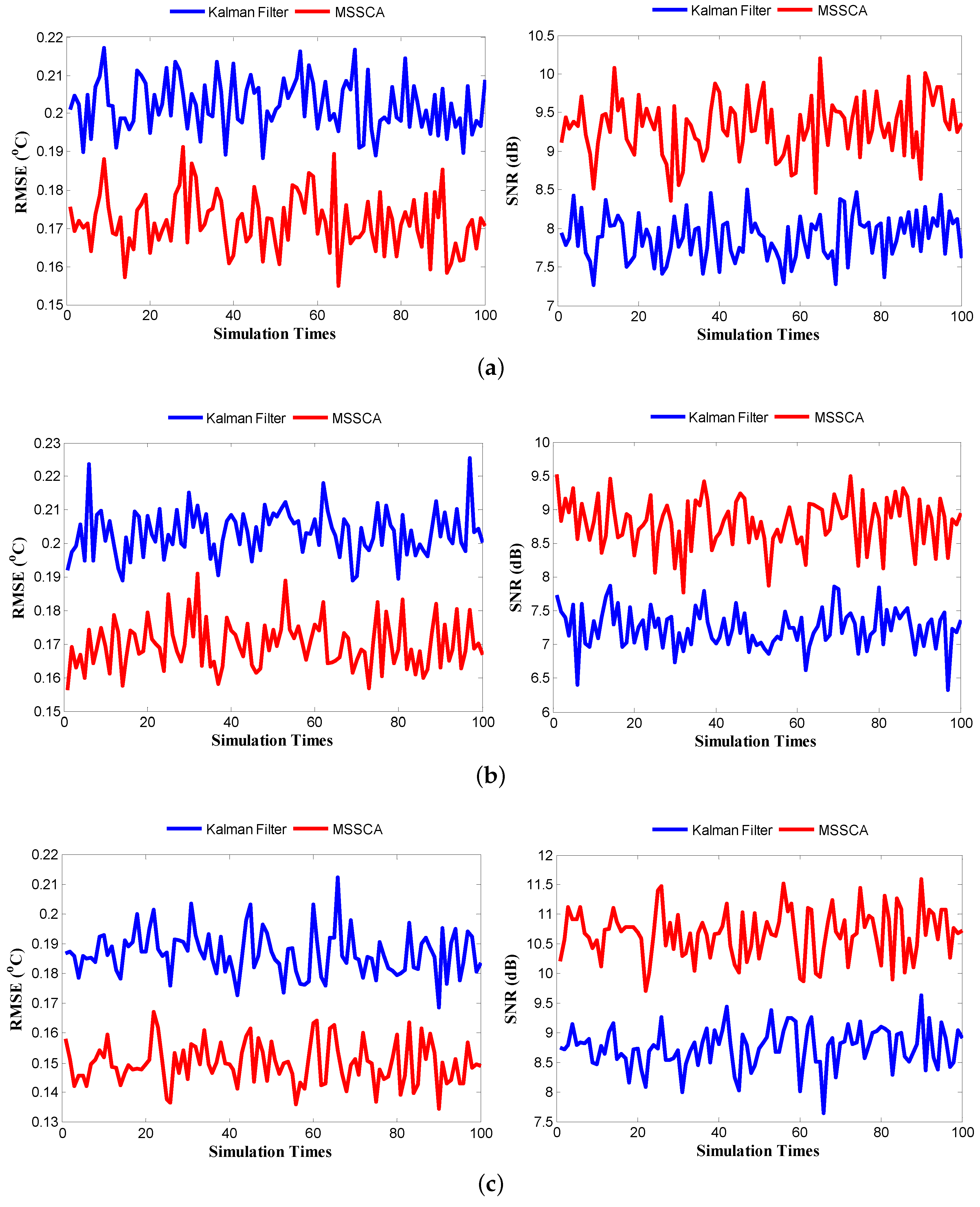
Figure 12 highlights the temperature tracking results of three sensors running the gamess benchmark. The standard deviation of the is set to be 5% of its mean value. The results of other benchmarks are similar. There are four different color curves plotted in the figure for each sensor: actual temperatures, noisy sensor readings, Kalman filter-corrected temperatures, and MSSCA-corrected temperatures. The simulation lasts for 51 s, and contains 3000 sample points, i.e., the sampling interval is 17 ms. From the results, it can be observed that the predicted temperatures using the MSSCA are much closer to the actual temperatures than those using the Kalman filter. In addition, the comparison results of the root-mean-square error (RMSE) and the signal-to-noise ratio (SNR) generated from the Kalman filter and MSSCA are shown in Figure 13. Experiments are performed with 100 time instances. From the results, it can be seen that the prediction performance of the MSSCA is clearly superior to that of the Kalman filter, with a lower RMSE and a higher SNR under all three sensors. Furthermore, an intuitive comparison of the prediction accuracy for different benchmarks is given in Figure 14. In Figure 14b (see the dealII benchmark), the RMSE of MSSCA can be reduced by 0.6 C (from 0.8 C to 0.2 C) relative to the noisy sensor readings. In Figure 14a (see the gobmk benchmark), the SNR of MSSCA is increased by 14.1 dB (from −3.8 dB to 10.3 dB) compared with the original sensor readings.
The results of average prediction accuracy under different noise standard deviations are reported in Table 3. Comparing the results, it can be observed that the MSSCA still exhibits superior prediction performance even if the noise standard deviation increases. In the case of 10% noise standard deviation, MSSCA can obtain a 1.2 C reduction in RMSE and a 15.8 dB increment in SNR compared with assuming the sensor readings to be ideal. Compared with Kalman filter, the average prediction accuracy increments of the MSSCA are reported in Table 4. As seen in Table 4, our MSSCA can achieve a 17.9% reduction in RMSE and a 45.8% increment in SNR. Note that the results of improvement for three sensors are slightly different. This is because the trends in temperature variation and the characteristics of observation data for different sensors lead to different degrees of improvement for prediction performance.
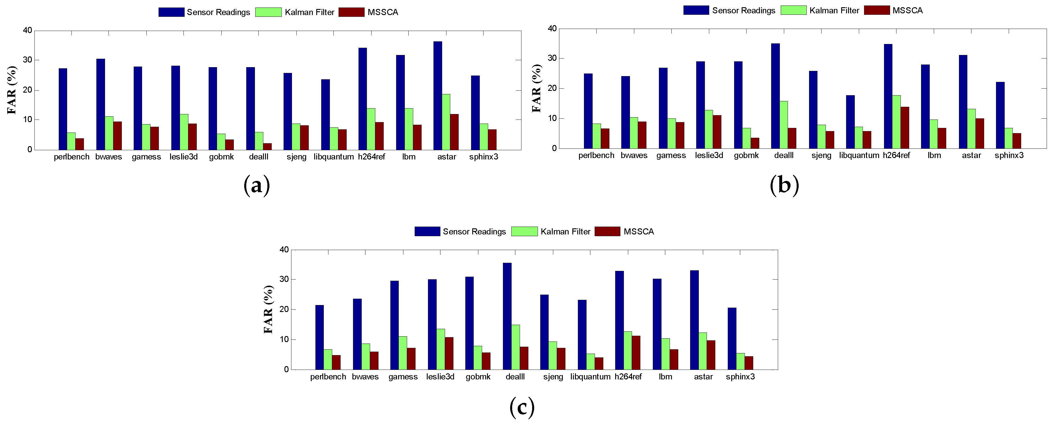
Another potential impact on DTM is the false alarm rate (FAR) [48], which is derived from two emergencies, i.e., missed and fake. The former indicates that the actual temperatures have exceeded the threshold temperature, but the estimated temperatures are still below it, and vice versa for the latter. The FAR comparison for different benchmarks is depicted in Figure 15, and the average results under different noise standard deviations are summarized in Table 5. In our case, the temperature threshold is set to 95% of the maximum temperature for each benchmark, where DTM will be triggered to cut down the frequencies. As seen in Table 5, MSSCA can achieve a 28.6% reduction in FAR as compared to the noisy sensor observations. The results clearly demonstrate that if our MSSCA is used to perform the temperature estimation, the performance of DTM can be significantly improved. This is because DTM mechanisms (e.g., dynamic voltage and frequency scaling (DVFS)) can be triggered to adjust the voltages, frequencies, and fan speeds at more appropriate times.
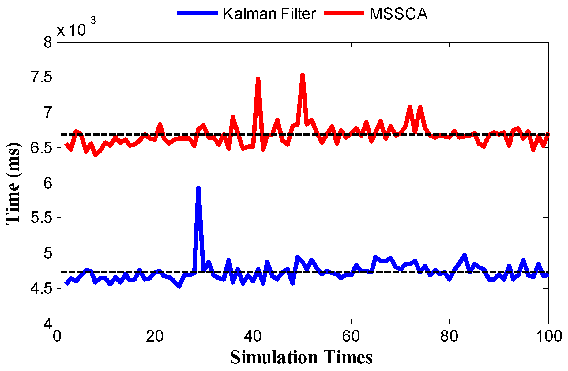
For each sensor calibration, the execution time comparison between the Kalman filter and the MSSCA is shown in Figure 16. Although the Kalman filter is clearly faster than the MSSCA, it can still achieve on-line temperature estimation. This is because the average execution time of the MSSCA (about 0.0066 ms) is obviously shorter than the sampling interval (17 ms). The requirement for our temperature estimation technique to be exploited by a processor is that additional memory is needed to store the correlation coefficients among all the available sensors.
6. Conclusions
In this paper, the problem of accurately estimating the temperatures for noisy thermal sensors is solved. We first analyze the noise characteristics of on-chip thermal sensors based on the ring oscillator structure and utilize the polynomial fitting technique to establish the non-linear relationship between the sensor temperature and output frequency of ring oscillator. On this basis, a smoothing filter-based Kalman prediction technique is proposed to correct the temperatures of on-die sensors in real time. Besides, a multi-sensor synergistic calibration algorithm (MSSCA) is proposed to improve the simultaneous prediction accuracy of multiple sensors. To evaluate the performance of our predictions, an infrared imaging-based temperature measurement technique is also proposed to capture the thermal traces of an AMD quad-core processor. Simulation results show that the proposed calibration scheme can achieve an around 1.2 C reduction in RMSE, a 15.8 dB increment in SNR, and a 28.6% reduction in FAR, as compared to the original sensor readings. Our approach will assist DTM mechanisms to achieve accurate temperature estimations in response to inaccuracies caused by fabrication randomness and environmental variation.
Acknowledgments
This work was supported by the National Natural Science Foundation of China under Grant 61501377.
Author Contributions
X.L., X.O. and Z.L. conceived the idea and designed the experiments. X.L. and H.W. constructed the infrared temperature measurement system and analyzed the obtained data. X.L. and X.O. analyzed the experimental results. W.Z. and Z.D. proposed the research topic and supervised the research. X.L. wrote the paper and discussed the contents.
Conflicts of Interest
The authors declare no conflict of interest.
References
- Mirtar, A.; Dey, S.; Raghunathan, A. Joint Work and Voltage/Frequency Scaling for Quality-Optimized Dynamic Thermal Management. IEEE Trans. Very Larg. Scale Integr. (VLSI) Syst. 2015, 23, 1017–1030. [Google Scholar] [CrossRef]
- Teravainen, S.; Haghbayan, M.-H.; Rahmani, A.-M.; Liljeberg, P.; Tenhunen, H. Software-Based On-Chip Thermal Sensor Calibration for DVFS-enabled Many-core Systems. In Proceedings of the IEEE International Symposium on Defect and Fault Tolerance in VLSI and Nanotechnology Systems (DFTS), Amherst, MA, USA, 12–14 October 2015; pp. 35–40. [Google Scholar]
- Mahfuzul Islam, A.K.M.; Shiomi, J.; Ishihara, T.; Onodera, H. Wide-Supply-Range All-Digital Leakage Variation Sensor for On-Chip Process and Temperature Monitoring. IEEE J. Solid-State Circuits 2015, 50, 2475–2490. [Google Scholar] [CrossRef]
- Shi, B.; Zhang, Y.; Srivastava, A. Dynamic Thermal Management under Soft Thermal Constraints. IEEE Trans. Very Larg. Scale Integr. (VLSI) Syst. 2013, 21, 2045–2054. [Google Scholar] [CrossRef]
- Chen, K.; Chang, E.; Li, H.; Wu, A. RC-Based Temperature Prediction Scheme for Proactive Dynamic Thermal Management in Throttle-Based 3D NoCs. IEEE Trans. Parallel Distrib. Syst. 2015, 26, 206–218. [Google Scholar] [CrossRef]
- Shafique, M.; Gnad, D.; Garg, S.; Henkel, J. Variability-Aware Dark Silicon Management in On-Chip Many-Core Systems. In Proceedings of the 2015 Design, Automation & Test in Europe Conference & Exhibition (DATE), Grenoble, France, 9–13 March 2015; pp. 387–392. [Google Scholar]
- Gnad, D.; Shafique, M.; Kriebel, F.; Rehman, S.; Sun, D.; Henkel, J. Hayat: Harnessing Dark Silicon and Variability for Aging Deceleration and Balancing. In Proceedings of the 52nd Design Automation Conference (DAC), San Francisco, CA, USA, 8–12 June 2015; pp. 1–6. [Google Scholar]
- Khdr, H.; Pagani, S.; Shafique, M.; Henkel, J. Thermal Constrained Resource Management for Mixed ILP-TLP Workloads in Dark Silicon Chips. In Proceedings of the 52nd Design Automation Conference (DAC), San Francisco, CA, USA, 8–12 June 2015; pp. 1–6. [Google Scholar]
- Khdr, H.; Pagani, S.; Sousa, E.; Lari, V.; Pathania, A.; Hannig, F.; Shafique, M.; Teich, J.; Henkel, J. Power Density-Aware Resource Management for Heterogeneous Tiled Multicores. IEEE Trans. Comput. 2017, 66, 488–501. [Google Scholar] [CrossRef]
- McGowen, R.; Poirier, C.A.; Bostak, C.; Ignowski, J.; Millican, M.; Parks, W.H.; Naffziger, S. Power and Temperature Control on a 90-nm Itanium Family Processor. IEEE J. Solid-State Circuits 2006, 41, 229–237. [Google Scholar] [CrossRef]
- Nakajima, M.; Kondo, H.; Okumura, N.; Masui, N.; Takata, Y.; Nasu, T.; Takata, H.; Higuchi, T.; Sakugawa, M.; Yoneda, H.; et al. Design of a Multi-Core SoC with Configurable Heterogeneous 9 CPUs and 2 Matrix Processors. In Proceedings of the IEEE Symposium on VLSI Circuits, Kyoto, Japan, 14–16 June 2007; pp. 14–15. [Google Scholar]
- Duarte, D.E.; Geannopoulos, G.; Mughal, U.; Wong, K.L.; Taylor, G. Temperature Sensor Design in a High Volume Manufacturing 65 nm CMOS Digital Process. In Proceedings of the IEEE Custom Integrated Circuits Conference (CICC ’07), San Jose, CA, USA, 16–19 September 2007; pp. 221–224. [Google Scholar]
- Sakran, N.; Yuffe, M.; Mehalel, M.; Doweck, J.; Knoll, E.; Kovacs, A. The Implementation of the 65 nm Dual-Core 64b Merom Processor. In Proceedings of the IEEE International Solid-State Circuits Conference (ISSCC 2007) Digest of Technical Papers, San Francisco, CA, USA, 11–15 February 2007; pp. 106–107. [Google Scholar]
- Dorsey, J.; Searles, S.; Ciraula, M.; Johnson, S.; Bujanos, N.; Wu, D.; Braganza, M.; Meyers, S.; Fang, E.; Kumar, R. An Integrated Quad-Core Opteron Processor. In Proceedings of the IEEE International Solid-State Circuits Conference (ISSCC 2007) Digest of Technical Papers, San Francisco, CA, USA, 11–15 February 2007; pp. 102–103. [Google Scholar]
- Floyd, M.S.; Ghiasi, S.; Keller, T.W.; Rajamani, K.; Rawson, F.L.; Rubio, J.C.; Ware, M.S. System power management support in the IBM POWER6 microprocessor. IBM J. Res. Dev. 2007, 51, 733–746. [Google Scholar] [CrossRef]
- Saneyoshi, E.; Nose, K.; Kajita, M.; Mizuno, M. A 1.1 V 35 μm × 35 μm thermal sensor with supply voltage sensitivity of 2 °C/10%-supply for thermal management on the SX-9 supercomputer. In Proceedings of the IEEE Symposium on VLSI Circuits, Honolulu, HI, USA, 18–20 June 2008; pp. 152–153. [Google Scholar]
- Kumar, R.; Hinton, G. A Family of 45 nm IA Processors. In Proceedings of the IEEE International Solid-State Circuits Conference (ISSCC 2009) Digest of Technical Papers, San Francisco, CA, USA, 8–12 February 2009; pp. 58–59. [Google Scholar]
- Kuppuswamy, R.; Sawant, S.R.; Balasubramanian, S.; Kaushik, P.; Natarajan, N.; Gilbert, J.D. Over One Million TPCC with a 45 nm 6-Core Xeon® CPU. In Proceedings of the IEEE International Solid-State Circuits Conference (ISSCC 2009) Digest of Technical Papers, San Francisco, CA, USA, 8–12 February 2009; pp. 70–71. [Google Scholar]
- Floyd, M.; Allen-Ware, M.; Rajamani, K.; Brock, B.; Lefurgy, C.; Drake, A.J.; Pesantez, L.; Gloekler, T.; Tierno, J.A.; Bose, P.; et al. Introducing the Adaptive Energy Management Features of the Power7 Chip. IEEE Micro 2011, 31, 60–75. [Google Scholar] [CrossRef]
- Dighe, S.; Gupta, S.; De, V.; Vangal, S.; Borkar, N.; Borkar, S.; Roy, K. A 45 nm 48-core IA processor with Variation-Aware Scheduling and Optimal Core Mapping. In Proceedings of the IEEE Symposium on VLSI Circuits (VLSIC), Honolulu, HI, USA, 15–17 June 2011; pp. 250–251. [Google Scholar]
- Fluhr, E.J.; Friedrich, J.; Dreps, D.; Zyuban, V.; Still, G.; Gonzalez, C.; Hall, A.; Hogenmiller, D.; Malgioglio, F.; Nett, R.; et al. 5.1 POWER8TM: A 12-Core Server-Class Processor in 22 nm SOI with 7.6 Tb/s Off-Chip Bandwidth. In Proceedings of the IEEE International Solid-State Circuits Conference (ISSCC 2014) Digest of Technical Papers, San Francisco, CA, USA, 9–13 February 2014; pp. 96–97. [Google Scholar]
- Remarsu, S.; Kundu, S. On process variation tolerant low cost thermal sensor design in 32 nm CMOS technology. In Proceedings of the ACM Great Lakes Symposium on VLSI, Boston Area, MA, USA, 10–12 May 2009; pp. 487–492. [Google Scholar]
- Yun, B.; Shin, K.G.; Wang, S. Predicting Thermal Behavior for Temperature Management in Time-Critical Multicore Systems. In Proceedings of the Real-Time and Embedded Technology and Applications Symposium (RTAS), Philadelphia, PA, USA, 9–11 April 2013; pp. 185–194. [Google Scholar]
- Beneventi, F.; Bartolini, A.; Tilli, A.; Benini, L. An Effective Gray-Box Identification Procedure for Multicore Thermal Modeling. IEEE Trans. Comput. 2014, 63, 1097–1110. [Google Scholar]
- Pagani, S.; Chen, J.-J.; Shafique, M.; Henkel, J. MatEx: Efficient Transient and Peak Temperature Computation for Compact Thermal Models. In Proceedings of the Design, Automation & Test in Europe Conference & Exhibition (DATE), Grenoble, France, 9–13 March 2015; pp. 1515–1520. [Google Scholar]
- Nowroz, A.N.; Cochran, R.; Reda, S. Thermal Monitoring of Real Processors: Techniques for Sensor Allocation and Full Characterization. In Proceedings of the 47th Design Automation Conference (DAC), Anaheim, CA, USA, 13–18 June 2010; pp. 56–61. [Google Scholar]
- Reda, S.; Dev, K.; Belouchrani, A. Blind Identification of Thermal Models and Power Sources from Thermal Measurements. IEEE Sens. J. 2018, 18, 680–691. [Google Scholar] [CrossRef]
- Zhang, Y.; Srivastava, A. Accurate Temperature Estimation Using Noisy Thermal Sensors for Gaussian and Non-Gaussian Cases. IEEE Trans. Very Larg. Scale Integr. (VLSI) Syst. 2011, 19, 1617–1626. [Google Scholar] [CrossRef]
- Lu, S.; Tessier, R.; Burleson, W. Dynamic On-Chip Thermal Sensor Calibration Using Performance Counters. IEEE Trans. Comput.-Aided Des. Integr. Circuits Syst. 2014, 33, 853–866. [Google Scholar] [CrossRef]
- Fu, Y.; Li, L.; Wang, K.; Zhang, C. Kalman Predictor-Based Proactive Dynamic Thermal Management for 3D NoC Systems with Noisy Thermal Sensors. IEEE Trans. Comput.-Aided Des. Integr. Circuits Syst. 2017, 36, 1869–1882. [Google Scholar] [CrossRef]
- Sharifi, S.; Liu, C.; Rosing, T.S. Accurate Temperature Estimation for Efficient Thermal Management. In Proceedings of the International Symposium on Quality Electronic Design (ISQED), San Jose, CA, USA, 17–19 March 2008; pp. 137–142. [Google Scholar]
- Sharifi, S.; Rosing, T.S. Accurate Direct and Indirect On-Chip Temperature Sensing for Efficient Dynamic Thermal Management. IEEE Trans. Comput.-Aided Des. Integr. Circuits Syst. 2010, 29, 1586–1599. [Google Scholar] [CrossRef]
- Lefebvre, C.A.; Rubio, L.; Montero, J.L. Digital Thermal Sensor Based on Ring-Oscillators in Zynq SoC Technology. In Proceedings of the International Workshop on Thermal Investigations of ICs and Systems (THERMINIC), Budapest, Hungary, 21–23 September 2016; pp. 276–278. [Google Scholar]
- Datta, B.; Burleson, W. Low-Power and Robust On-Chip Thermal Sensing Using Differential Ring Oscillators. In Proceedings of the 50th Midwest Symposium on Circuits and Systems (MWSCAS), Montreal, QC, Canada, 5–8 August 2007; pp. 29–32. [Google Scholar]
- Rosinha, J.B.; de Almeida, S.J.M.; Bermudez, J.C.M. A New Kernel Kalman Filter Algorithm for Estimating Time-Varying Nonlinear Systems. In Proceedings of the IEEE International Symposium on Circuits and Systems (ISCAS), Baltimore, MD, USA, 28–31 May 2017; pp. 1–4. [Google Scholar]
- Einicke, G.A. Smoothing, Filtering and Prediction-Estimating The Past, Present and Future; InTech: Rijeka, Croatia, 2012. [Google Scholar]
- Fu, Y.; Li, L.; Pan, H.; Wang, K.; Han, F.; Lin, J. Accurate Runtime Thermal Prediction Scheme for 3D NoC Systems with Noisy Thermal Sensors. In Proceedings of the IEEE International Symposium on Circuits and Systems (ISCAS), Montreal, QC, Canada, 22–25 May 2016; pp. 1198–1201. [Google Scholar]
- Friedberg, P.; Cao, Y.; Cain, J.; Wang, R.; Rabaey, J.; Spanos, C. Modeling Within-Die Spatial Correlation Effects for Process-Design Co-Optimization. In Proceedings of the Sixth International Symposium on Quality of Electronic Design (ISQED), San Jose, CA, USA, 21–23 March 2005; pp. 516–521. [Google Scholar]
- Hargreaves, B.; Hult, H.; Reda, S. Within-die Process Variations: How Accurately Can They Be Statistically Modeled? In Proceedings of the Asia and South Pacific Design Automation Conference (ASPDAC), Seoul, Korea, 21–24 March 2008; pp. 524–530. [Google Scholar]
- Xiong, J.; Zolotov, V.; He, L. Robust Extraction of Spatial Correlation. IEEE Trans. Comput.-Aided Des. Integr. Circuits Syst. 2007, 26, 619–631. [Google Scholar] [CrossRef]
- Brooks, D.; Tiwari, V.; Martonosi, M. Wattch: A Framework for Architectural-Level Power Analysis and Optimizations. In Proceedings of the 27th International Symposium on Computer Architecture, Vancouver, BC, Canada, 19 May 2000; pp. 83–94. [Google Scholar]
- Huang, W.; Ghosh, S.; Velusamy, S.; Sankaranarayanan, K.; Skadron, K.; Stan, M.R. HotSpot: A Compact Thermal Modeling Methodology for Early-Stage VLSI Design. IEEE Trans. Very Larg. Scale Integr. (VLSI) Syst. 2006, 14, 501–513. [Google Scholar] [CrossRef]
- Reda, S.; Cochran, R.; Nowroz, A.N. Improved Thermal Tracking for Processors Using Hard and Soft Sensor Allocation Techniques. IEEE Trans. Comput. 2011, 60, 841–851. [Google Scholar] [CrossRef]
- Ardestani, E.K.; Mesa-Martínez, F.J.; Renau, J. Cooling Solutions for Processor Infrared Thermography. In Proceedings of the 26th Annual IEEE Semiconductor Thermal Measurement and Management Symposium, Santa Clara, CA, USA, 21–25 February 2010; pp. 187–190. [Google Scholar]
- Ardestani, E.K.; Mesa-Martínez, F.J.; Southern, G.; Ebrahimi, E.; Renau, J. Sampling in Thermal Simulation of Processors: Measurement, Characterization, and Evaluation. IEEE Trans. Comput.-Aided Des. Integr. Circuits Syst. 2013, 32, 1187–1200. [Google Scholar] [CrossRef]
- Zou, Q.; Yue, J.; Segee, B.; Zhu, Y. Temporal Characterization of SPEC CPU2006 Workloads: Analysis and Synthesis. In Proceedings of the IEEE International Performance Computing and Communications Conference (IPCCC), Austin, TX, USA, 1–3 December 2012; pp. 11–20. [Google Scholar]
- Dev, K.; Nowroz, A.N.; Reda, S. Power Mapping and Modeling of Multi-core Processors. In Proceedings of the IEEE International Symposium on Low Power Electronics and Design (ISLPED), Beijing, China, 4–6 September 2013; pp. 39–44. [Google Scholar]
- Li, X.; Jiang, W.; Zhou, W. Optimising thermal sensor placement and thermal maps reconstruction for microprocessors using simulated annealing algorithm based on PCA. IET Circuits Devices Syst. 2016, 10, 463–472. [Google Scholar] [CrossRef]
Figure 1.
Trends in the number of embedded thermal sensors in VLSI systems.

Figure 2.
Structure of a typical ring oscillator.

Figure 3.
Results of the Monte Carlo (MC) simulation. (a) Probability density distribution of output frequencies under different temperatures; (b) Statistical histogram of output frequency distribution at the temperature of 70 C.
Figure 3.
Results of the Monte Carlo (MC) simulation. (a) Probability density distribution of output frequencies under different temperatures; (b) Statistical histogram of output frequency distribution at the temperature of 70 C.

Figure 4.
Flowchart of the proposed scheme for temperature estimation. MSSCA: multi-sensor synergistic calibration algorithm.
Figure 4.
Flowchart of the proposed scheme for temperature estimation. MSSCA: multi-sensor synergistic calibration algorithm.
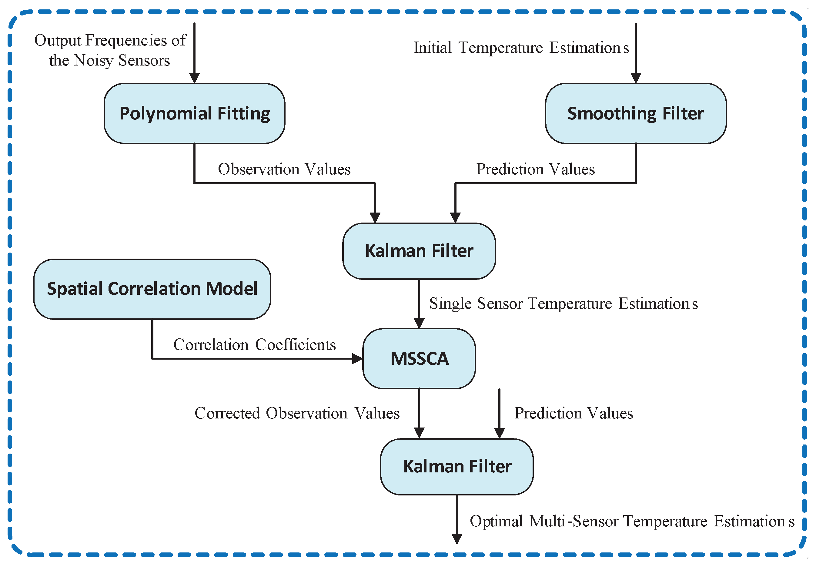
Figure 5.
Result of the polynomial fitting.

Figure 6.
Framework of the Kalman filter algorithm.
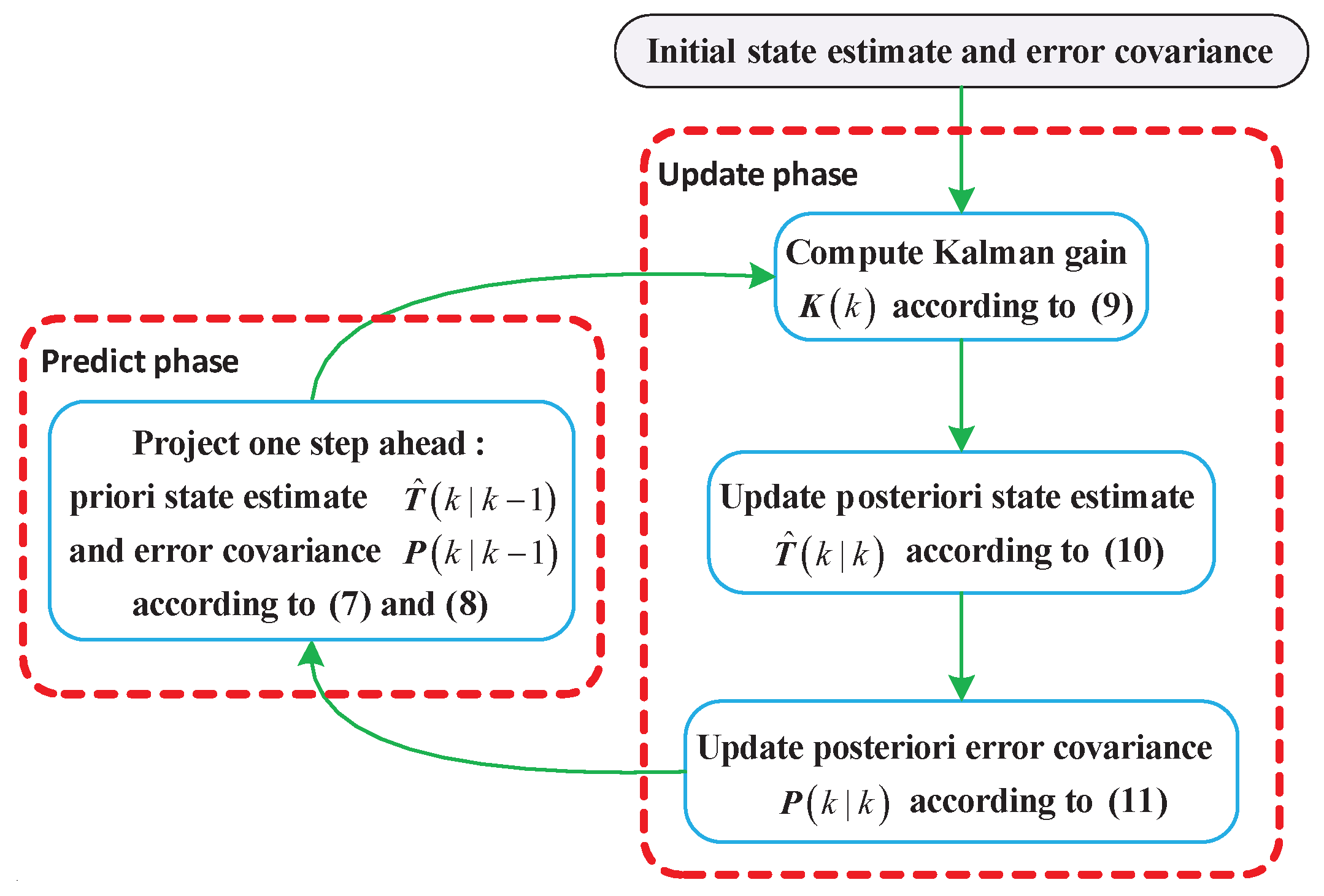
Figure 7.
Distribution of sensor locations and the corresponding temperature variations. (a) Distribution of sensor locations; (b) Thermal traces of different sensor locations.
Figure 7.
Distribution of sensor locations and the corresponding temperature variations. (a) Distribution of sensor locations; (b) Thermal traces of different sensor locations.
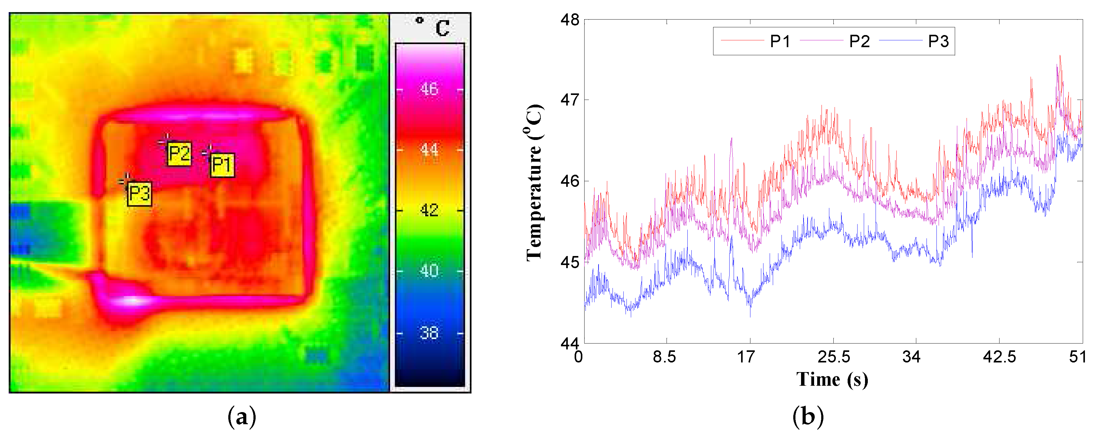
Figure 8.
Spatial correlation functions generated from Equation (12).
Figure 8.
Spatial correlation functions generated from Equation (12).

Figure 9.
Proposed infrared temperature measuring equipment. (a) Oil-based cooling system; (b) Infrared transparent heat sink.
Figure 9.
Proposed infrared temperature measuring equipment. (a) Oil-based cooling system; (b) Infrared transparent heat sink.
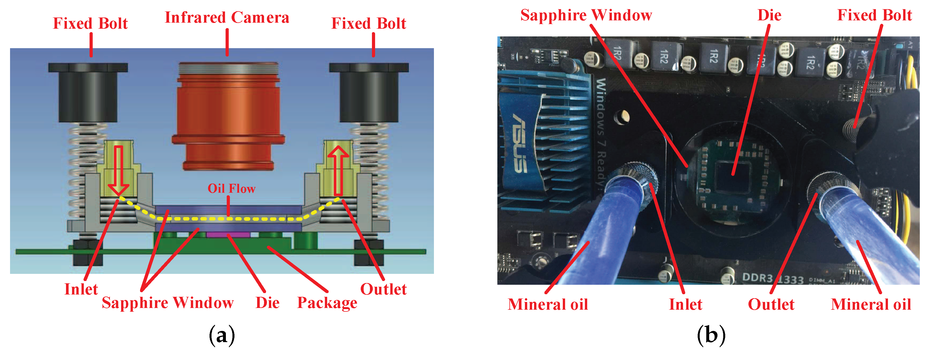
Figure 10.
Image of our experimental setup.

Figure 11.
Examples of thermal traces of different benchmarks on a quad-core AMD Athlon II X4 610e processor. (a) sjeng; (b) h264ref; (c) lbm; (d) leslie3d; (e) sphinx3; (f) dealII.
Figure 11.
Examples of thermal traces of different benchmarks on a quad-core AMD Athlon II X4 610e processor. (a) sjeng; (b) h264ref; (c) lbm; (d) leslie3d; (e) sphinx3; (f) dealII.
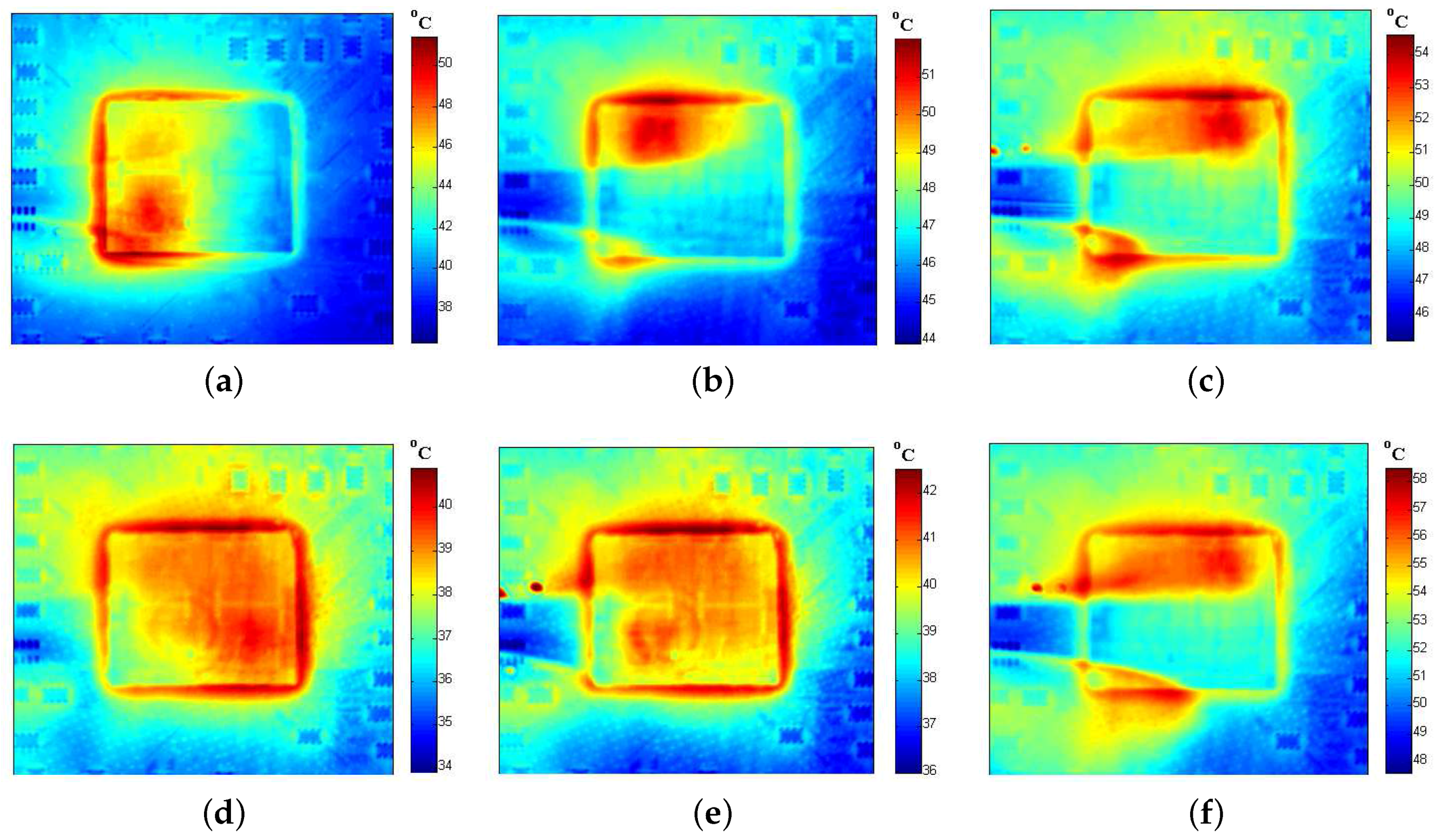
Figure 12.
Comparison of temperature tracking (over 51 s) for three sensors in Figure 7a running the gamess benchmark. Noise standard deviation is 5%. (a) P1 sensor; (b) P2 sensor; (c) P3 sensor. MSSCA: multi-sensor synergistic calibration algorithm.
Figure 12.
Comparison of temperature tracking (over 51 s) for three sensors in Figure 7a running the gamess benchmark. Noise standard deviation is 5%. (a) P1 sensor; (b) P2 sensor; (c) P3 sensor. MSSCA: multi-sensor synergistic calibration algorithm.

Figure 13.
Root-mean-square error (RMSE) and signal-to-noise ratio (SNR) generated from the Kalman filter and the MSSCA with 100 time instances for three sensors in Figure 7a running the gamess benchmark. Noise standard deviation is 5%. (a) P1 sensor; (b) P2 sensor; (c) P3 sensor.
Figure 13.
Root-mean-square error (RMSE) and signal-to-noise ratio (SNR) generated from the Kalman filter and the MSSCA with 100 time instances for three sensors in Figure 7a running the gamess benchmark. Noise standard deviation is 5%. (a) P1 sensor; (b) P2 sensor; (c) P3 sensor.

Figure 14.
Comparison of prediction accuracy for different benchmarks. Noise standard deviation is 5%. (a) P1 sensor; (b) P2 sensor; (c) P3 sensor.
Figure 14.
Comparison of prediction accuracy for different benchmarks. Noise standard deviation is 5%. (a) P1 sensor; (b) P2 sensor; (c) P3 sensor.
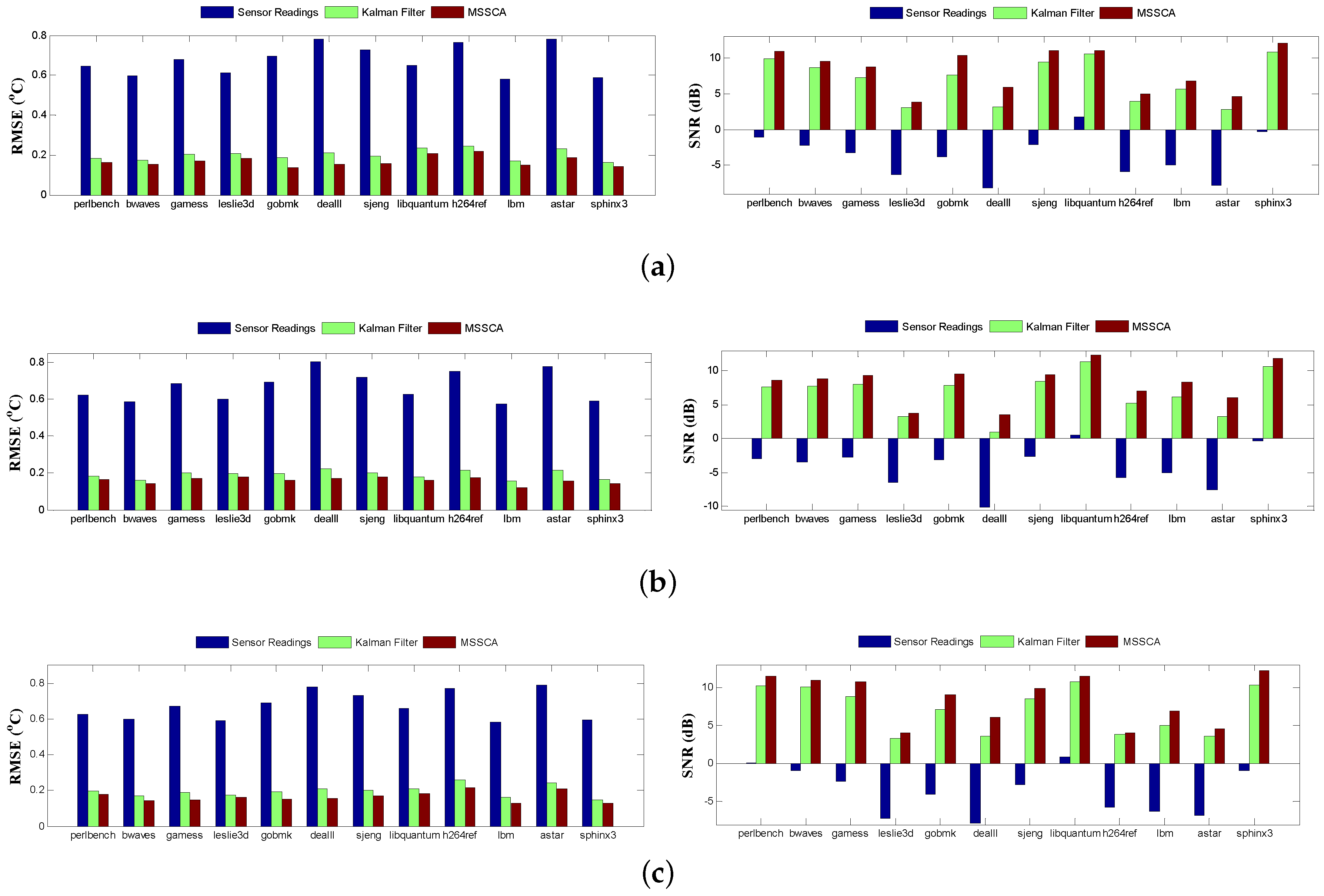
Figure 15.
Comparison of the false alarm rate (FAR) for different benchmarks. Noise standard deviation is 5%. (a) P1 sensor; (b) P2 sensor; (c) P3 sensor.
Figure 15.
Comparison of the false alarm rate (FAR) for different benchmarks. Noise standard deviation is 5%. (a) P1 sensor; (b) P2 sensor; (c) P3 sensor.

Figure 16.
Execution time comparison between the Kalman filter and the MSSCA.


Table 1.
Characteristics of the random variables.
| Parameters | (nm) | (nm) | (nm) | (v) | (v) | m2/(V·s) |
|---|---|---|---|---|---|---|
| Mean | 270 | 180 | 4.1 | 3 | 0.45 | 0.034 |
| Standard deviation | 5% | 6% | 3% | 5% | 4% | 2% |
Table 2.
Correlation coefficients among different sensors.
| Correlation | P1 | P2 | P3 |
|---|---|---|---|
| P1 | 1 | 0.8991 | 0.7134 |
| P2 | 0.8991 | 1 | 0.8808 |
| P3 | 0.7134 | 0.8808 | 1 |
Table 3.
Average prediction accuracy for different benchmarks.
| Standard Deviation | Sensor ID | RMSE () | SNR (dB) | ||||
|---|---|---|---|---|---|---|---|
| Sensor Readings | Kalman Filter | MSSCA | Sensor Readings | Kalman Filter | MSSCA | ||
| 5% | P1 | 0.6757 | 0.2006 | 0.1690 | −3.6697 | 6.8931 | 8.3156 |
| P2 | 0.6687 | 0.1913 | 0.1612 | −4.1133 | 6.7305 | 8.2271 | |
| P3 | 0.6734 | 0.1952 | 0.1651 | −3.6588 | 7.0747 | 8.4353 | |
| 10% | P1 | 1.3571 | 0.2776 | 0.2309 | −9.7271 | 4.0771 | 5.6569 |
| P2 | 1.3767 | 0.2672 | 0.2193 | −10.2051 | 3.8401 | 5.5996 | |
| P3 | 1.3527 | 0.2751 | 0.2301 | −9.7174 | 4.1676 | 5.6734 | |
Table 4.
Average prediction accuracy increment of the MSSCA compared with the Kalman filter.
| Standard Deviation | Sensor ID | RMSE () | SNR (dB) |
|---|---|---|---|
| MSSCA vs. Kalman Filter | MSSCA vs. Kalman Filter | ||
| 5% | P1 | −15.75% | +20.64% |
| P2 | −15.73% | +22.24% | |
| P3 | −15.42% | +19.23% | |
| 10% | P1 | −16.82% | +38.75% |
| P2 | −17.93% | +45.82% | |
| P3 | −16.36% | +36.13% |
Table 5.
Average FAR for different benchmarks.
| Standard Deviation | Sensor ID | FAR (%) | ||
|---|---|---|---|---|
| Sensor Readings | Kalman Filter | MSSCA | ||
| 5% | P1 | 28.7542 | 9.9867 | 7.1483 |
| P2 | 27.3608 | 10.4633 | 7.68583 | |
| P3 | 28.0150 | 9.8583 | 7.08583 | |
| 10% | P1 | 37.8958 | 13.6108 | 9.2775 |
| P2 | 36.9525 | 14.2808 | 10.1975 | |
| P3 | 37.2767 | 12.6075 | 8.8508 | |
© 2018 by the authors. Licensee MDPI, Basel, Switzerland. This article is an open access article distributed under the terms and conditions of the Creative Commons Attribution (CC BY) license (http://creativecommons.org/licenses/by/4.0/).
Share and Cite
MDPI and ACS Style
Li, X.; Ou, X.; Li, Z.; Wei, H.; Zhou, W.; Duan, Z. On-Line Temperature Estimation for Noisy Thermal Sensors Using a Smoothing Filter-Based Kalman Predictor. Sensors 2018, 18, 433. https://doi.org/10.3390/s18020433
AMA Style
Li X, Ou X, Li Z, Wei H, Zhou W, Duan Z. On-Line Temperature Estimation for Noisy Thermal Sensors Using a Smoothing Filter-Based Kalman Predictor. Sensors. 2018; 18(2):433. https://doi.org/10.3390/s18020433
Chicago/Turabian StyleLi, Xin, Xingtao Ou, Zhi Li, Henglu Wei, Wei Zhou, and Zhemin Duan. 2018. "On-Line Temperature Estimation for Noisy Thermal Sensors Using a Smoothing Filter-Based Kalman Predictor" Sensors 18, no. 2: 433. https://doi.org/10.3390/s18020433
Note that from the first issue of 2016, this journal uses article numbers instead of page numbers. See further details here.