Stress Prediction for Distributed Structural Health Monitoring Using Existing Measurements and Pattern Recognition

Harbin Institute of Technology (Shenzhen), Shenzhen 518055, China
*
Authors to whom correspondence should be addressed.
Sensors 2018, 18(2), 419; https://doi.org/10.3390/s18020419
Submission received: 31 October 2017
/
Revised: 26 January 2018
/
Accepted: 29 January 2018
/
Published: 1 February 2018
(This article belongs to the Special Issue Sensor Technologies for Health Monitoring of Composite Structures)
Abstract
:The stress in structural steel members is the most useful and directly measurable physical quantity to evaluate the structural safety in structural health monitoring, which is also an important index to evaluate the stress distribution and force condition of structures during structural construction and service phases. Thus, it is common to set stress as a measure in steel structural monitoring. Considering the economy and the importance of the structural members, there are only a limited number of sensors that can be placed, which means that it is impossible to obtain the stresses of all members directly using sensors. This study aims to develop a stress response prediction method for locations where there are insufficent sensors, using measurements from a limited number of sensors and pattern recognition. The detailed improved aspects are: (1) a distributed computing process is proposed, where the same pattern is recognized by several subsets of measurements; and (2) the pattern recognition using the subset of measurements is carried out by considering the optimal number of sensors and number of fusion patterns. The validity and feasibility of the proposed method are verified using two examples: the finite-element simulation of a single-layer shell-like steel structure, and the structural health monitoring of the space steel roof of Shenzhen Bay Stadium; for the latter, the anti-noise performance of this method is verified by the stress measurements from a real-world project.
1. Introduction
Structural stress distribution is a critical and directly-measurable parameter to evaluate structural safety [1] in which monitoring and prediction of the stress distribution of real-world structures is key to the application of structural health monitoring. A stress development prediction method was proposed to predict the stress development trend and provide a deterioration assessment for existing bridges [1]. Long-term monitoring data of dynamic strain were used for fatigue life assessment of steel bridges, where the strain measurement data from the Tsing Ma Bridge were used to verify the method [2]. The maximum stress of beam structures was measured during monitoring, and it was compared with the allowable stress and used to assess structural safety [3]. For such stress prediction methods, the critical problem is that the number of the sensors for stress monitoring is limited, although there is some research on the optimal placement of sensors to control the number of sensors in a reasonable range and ensure that the sensors provide the greatest efficiency. This is because the installation of sensor systems is expensive. Zhang proposed an optimal multi-type sensor placement method to reconstruct the structural responses. The method considered the measurement of structural response and was limited to a few locations [4]. In other words, sensors are arranged only on some key components, and then the stress of the entire structure is identified by the analysis method.
Based on the limited number of stress measurements, the prediction methods for stress distribution were researched and developed. A sensor-free stress estimation model was proposed to estimate the stress distribution of steel beam structures. The model considered the uncertain loads to which the building structure was exposed [5]. A Gaussian particle filtering algorithm was used to predict the dynamic extreme stress based on the monitoring data [6]. A Kalman filter method with a dynamic model of the structure was used to estimate the power spectral density of stresses at unmeasured locations based on the measurements at the limited locations [7]. A model-based state estimator was proposed to predict the stress measurements at arbitrary locations in the structure based on acceleration measurements [8,9,10]. Pattern identification was used to estimate the structural stresses based on stress measurements and displacement measurements [11]. Xu validated the effectiveness and practicability of the proposed multi-type sensor placement and response reconstruction method according to the good agreement of the reconstructed multi-type responses between the numerical studies and the experimental investigations [12]. Lu proposed an improved pattern recognition method, which selected more than one best pattern and used weighting parameters to obtain the synthesized estimated stress values [11]. Zhang presented a restoring method for spatial structural stress monitoring. That method can avoid the missing data using correlation among the measuring points [13]. It is obvious that stress monitoring is important for the structural safety assessment, and there is much research regarding the structural safety assessment using stress measurements and the prediction method for the stress values at the sensor-free placements. However, such methods just considered how to realize the stress prediction, where the prediction processes were all concentrated; in other words, such methods may be unusable if the measurements were partially missed or the central data-processing centre breaks down.
Some research has been based on function dispersion. Smarsly proposed an analytical redundancy approach to decentralized sensor fault detection by using artificial neural networks [14]. Sim presented a decentralized data aggregation approach for system identification based on the random decrement technique, which was used for wireless sensor networks and demonstrated its effectiveness by the accuracy of estimated modal properties and wireless data communication [15]. Lynch developed intelligent data-processing nodes by setting a signal-processing algorithm into sensors. This approach has been applied in the Alamosa Canyon Bridge in New Mexico [16]. Leng divided petroleum pipe software into two subsystems: a data management system and a data analysis system. The two systems work concurrently to complete a second pre-processing, data storage, and data analysis [17]. Gao [18] established a powerful structural health monitoring hardware platform and identified stress by a kind of distributed data acquisition system called ‘small concentrated’. Inaudi [19] introduced the monitoring of data standard management considering the difficulty in storing mass data. The research developed the decentralized functions in condensing mass measurements, data acquisition, and data pre-processing, where the effectiveness has already been proved partially. Furthermore, the structural health monitoring methods should be developed based on such decentralized functions to reduce the potential risks caused by sensor failure and to improve the operation efficiency caused by function concentration.
A stress prediction method in distributed processes is proposed. It is based on the limited stress measurements and pattern recognition method. The aim of the proposed method is to develop a stress prediction method that can be adaptive to the distributed sensor networks accompanying the decentralized functions. Here, we first propose a distributed algorithm based on pattern recognition, where the number of sensors and patterns is considered. Furthermore, simulation of the shell-like structure is performed to verify the effectiveness of the proposed method. In addition, measurements of a real-world structure are used to prove the proposed method by considering noise influences.
2. Distributed Algorithm Based on Pattern Recognition
Compared with only one pattern library using all the measurements, there are multiple pattern libraries that recognize stress in monitoring positions to achieve distributed operation. If one pattern library is simply being divided into some subparts, it can be helpful for improving the calculation efficiency, but not for precise recognition.
In this paper, the process of a distributed computing method based on pattern recognition is to establish multiple pattern libraries to recognize the same single pattern, and there are still two improved aspects: (1) information optimised from different pattern libraries, which is the optimization of the number of sensors, and (2) an optimal amount of fusion patterns chosen during a distributed-computing process and final fusion computation. The steps to the method are as follows: (1) sensors are divided into m subgroups; therefore, there will be subpattern-recognizing libraries and subtesting libraries; (2) for each subpattern recognition library and subtesting library, the optimal number of sensors is chosen for the calculation and fusion algorithm patterns; and (3) optimised fusion algorithm patterns are gathered into one total pattern library. Then, the stress prediction of unknown positions based on distributed computing and the pattern recognition method can be completed.
2.1. Measurements and Response to Be Recognized
The measurements collected from sensors can be represented as :
where is the time series of the measurement collected from the th sensor.
The response to be recognized can be represented as .
2.2. Distributed Subsets of Measurements
The measurements can be divided into subsets of measurements, which can be represented as , ,…, ,…, . The subset of measurements is represented as:
where ; is the number of measurements in the th subset of measurements. is the th measurements in the th subset of measurements.
2.3. Pattern Recognition Based on a Subset of Measurements
2.3.1. Sequenced Responses Based on the Correlation
The finite-element model of the structure is built first. It is used to calculate the structural responses at the locations of sensors and the location to be recognized. The calculated structural responses at the location of sensors and location to be recognized are represented as and , respectively, which has time steps and can be used to give the correlations between the responses at the location of sensors and the response at the location to be recognized. The correlation between the response at the location of sensors and the response at the location to be recognized is represented as :
The responses included in the th subsets can be sequenced by the value of correlation . The sequenced measurements can be represented as :
where .
2.3.2. Error Analysis on Different Numbers of Sensors and Patterns
The input of the traditional pattern recognition method is , and the output of the traditional pattern recognition method is .
If the number of sensors is considered, the input of the advanced pattern recognition method can be , ,…, ,…, , respectively:
where ; represents the number of sensors in th subset.
If the number of recognized patterns is considered, the output of the advanced pattern recognition method can be , ,…, ,…, , respectively:
where ; represents the number of well-matched patterns, and represents the th well-matched pattern.
The approach degree between well-matched patterns and pattern to be recognized is represented by vector :
If the number of patterns is considered, the output of the advanced pattern recognition method can be , ,…, ,…, , respectively:
The recognition error with the different number of sensors and the different number of patterns can be represented as:
where is the determined number of sensors, and is the determined number of patterns.
The input of such a best pattern library for the th subset of measurements is:
The output of such a best pattern library for the th subset of measurements is:
The predicted value for the pattern to be recognized is:
The predicted values using subsets of measurements can be given as , ,…, ,…, , respectively.
2.4. Pattern Recognition Based on Gross Sets of Measurements
The gross set of measurements based on the input of each best pattern library for subsets of measurements can be represented as:
The predicted value by considering the best number of sensors and patterns is:
where and are the best number of sensors and patterns when the gross set of measurements is used.
3. The Simulation on the Stress Recognition of Shell-Like Structures
3.1. The Main Parameters of Shell-Like Structures
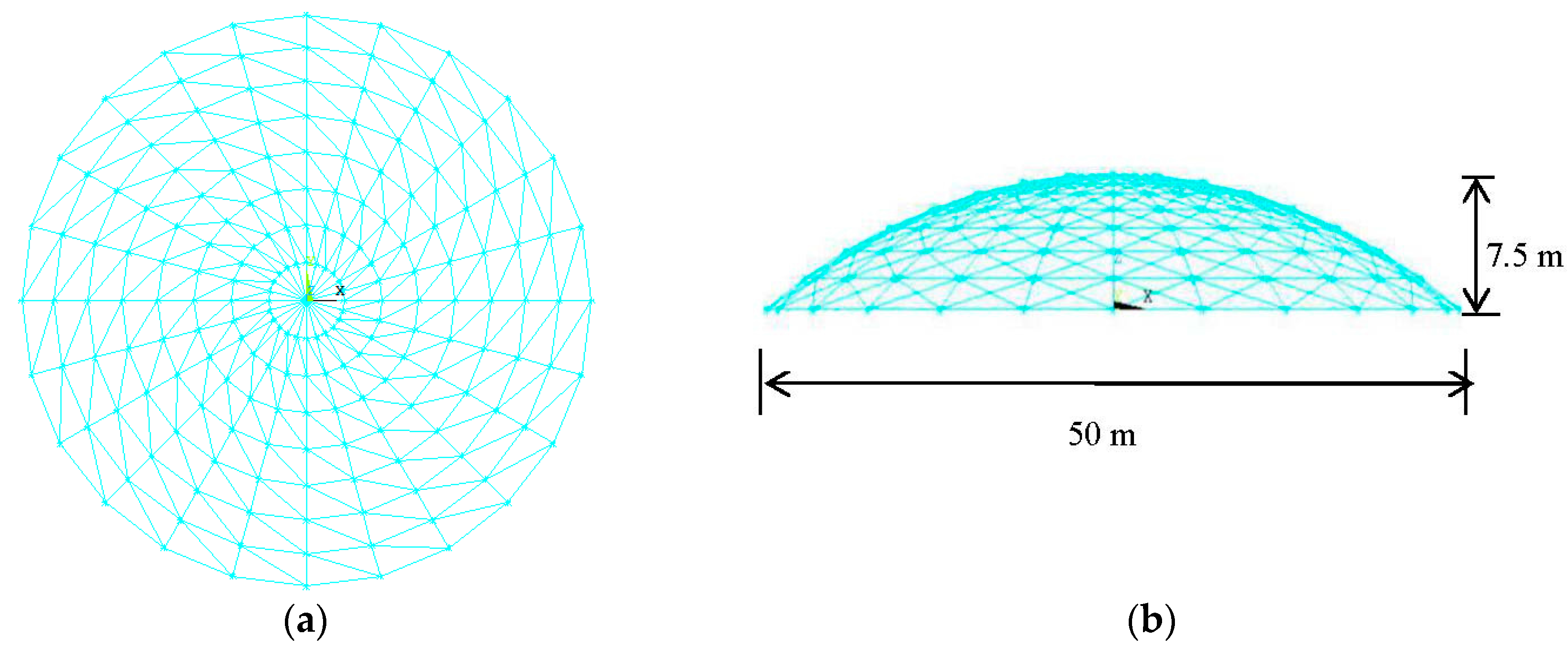
The finite-element model is built based on the Schwedler shell-like structure [20], which is shown in Figure 1. The shell-like structure is 50 m long, 50 m wide, and 7.5 m high. The uniform mass is 200 Kg/m2. The material of the steel members is Q235, the elastic modulus is , the Poisson ratio is 0.3, and the damping ratio is 0.02 in Rayleigh damping. The section of the member in the radial direction is 133 4, while the section of the members in the circle direction and diagonal direction is 127 3. The Poisson ratio is 0.3. The type of support is a fixed-hinge support.
In this finite-element method calculation, the Karman spectrum is selected to simulate the along-wind fluctuating wind spectrum, while the calculation equation proposed by Panofsky is selected to simulate the vertical-wind fluctuating wind spectrum. The formulas are shown below:
where is the fluctuated wind power spectrum, is the average wind speed at the height of z, is the fluctuated angular frequency, is the roughness coefficient on the ground, , is the roughness length, and is the Kaman constant.
3.2. Layout of Sensors
A variable coefficient (VC), a kind of parameter used for measuring and reflecting discrete levels of a set of data, is used to determine the placement of sensors, which is represented as:
where is the VC of the items of components, is the standard deviation of the items of components, and is the average value of the items of components.
A time-domain dynamic analysis of this finite-element method is carried out by setting a fluctuating wind load whose average speed reaches 15 m/s. The total loading time is 10 min and 6000 substeps. For each step, the combined stresses of axial stress and bending stress in Y+ at 1/4 length of the members are extracted. According to the values of VC with descending order, the first 26 members are chosen to locate the sensors and extract the stresses; the number of the members are 153, 152, 154, 168, 151, 155, 150, 129, 128, 156, 130, 127, 149, 164, 163, 131, 165, 162, 126, 161, 166, 132, 105, 140, 157, and 139. According to the value of VC with descending order, the first eight points are chosen to extract the displacements, and the number of the members are 2, 12, 13, 14, 15, 16, 17, and 18.
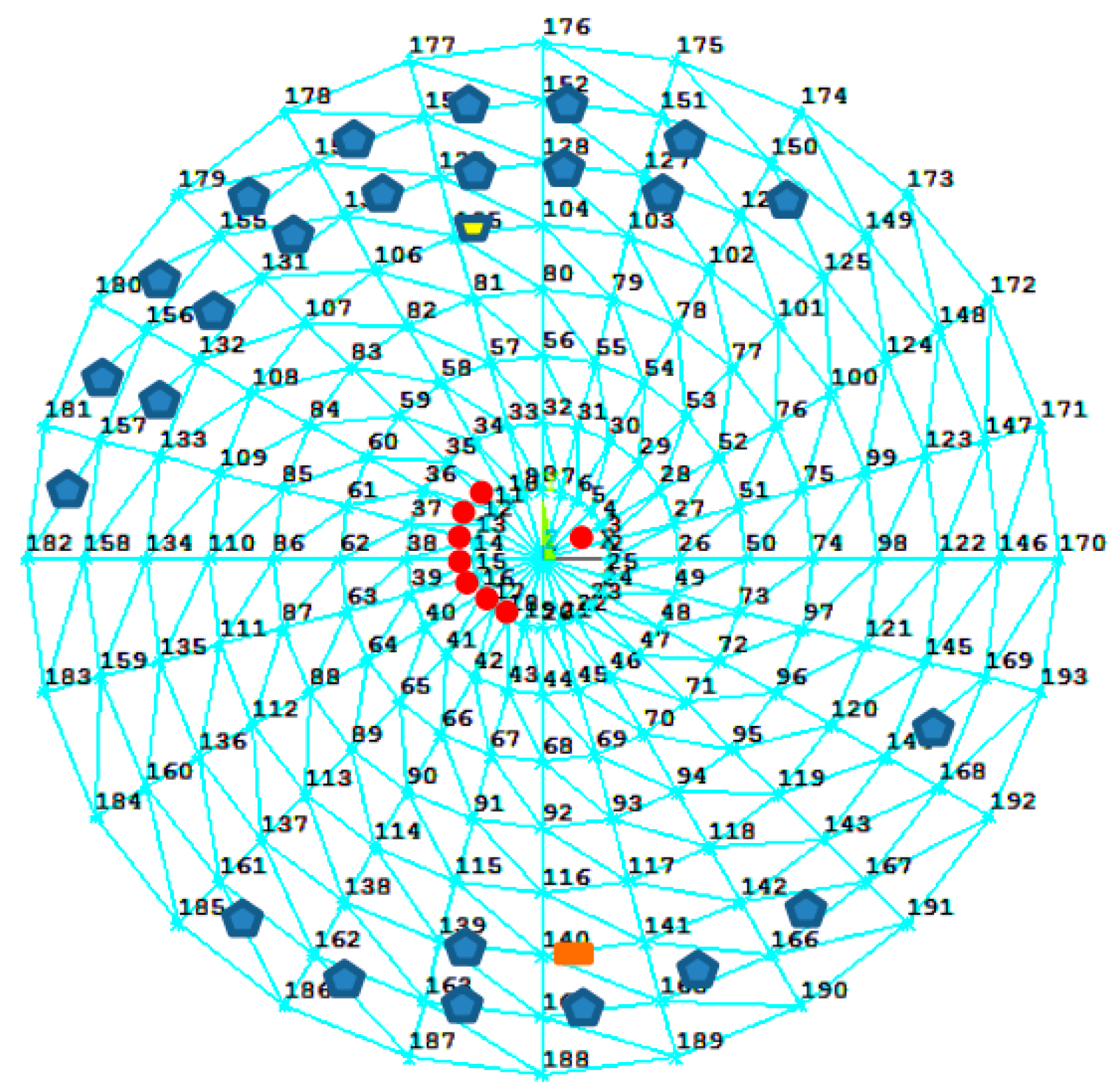
Considering the values of VC, stress changing, and average stress, the members with No. 105 and No. 140 are selected as the stress of members to be identified, which are denoted as Position A and Position B, respectively. Those positions, the members for extracting stresses, and the points for extracting displacements are shown in Figure 2.
3.3. Pattern Sets and Subsets of Measurement
A fluctuated wind load whose average value increases from 5 m/s to 50 m/s (5 m/s for each step) is simulated for the finite-element method analysis. In addition, the stresses and displacements are extracted from the finite-element method every 0.1 s, and the total analysis time is 10 min; that is, the stresses and displacements extracted from the finite-element method analysis are 6000 time steps. Furthermore, the data are separated into the pattern library, testing library, and observed library. The stress and displacement responses from the first time step and those in every three time steps are the data in the pattern library; there are a total of 15,000 patterns. The stress and displacement responses from the second time step and those in every 120 time steps are the data in the testing library; there are a total of 500 patterns. The stress and displacement responses from the third time step and those in every 600 time steps are the data in the observed library, and there are 100 patterns. The subsets of measurement are given in Table 1.
3.4. Determination of the Optimal Number of Sensors and Patterns
There are four subsets of measurement, while the determination of the optimal number of sensors and patterns is illustrated using Subset 1.
(1) The correlation between the responses of the points in No. 1 subset of measurement and the stresses of Position A can be calculated by Equation (4), sorted and shown in Table 2.
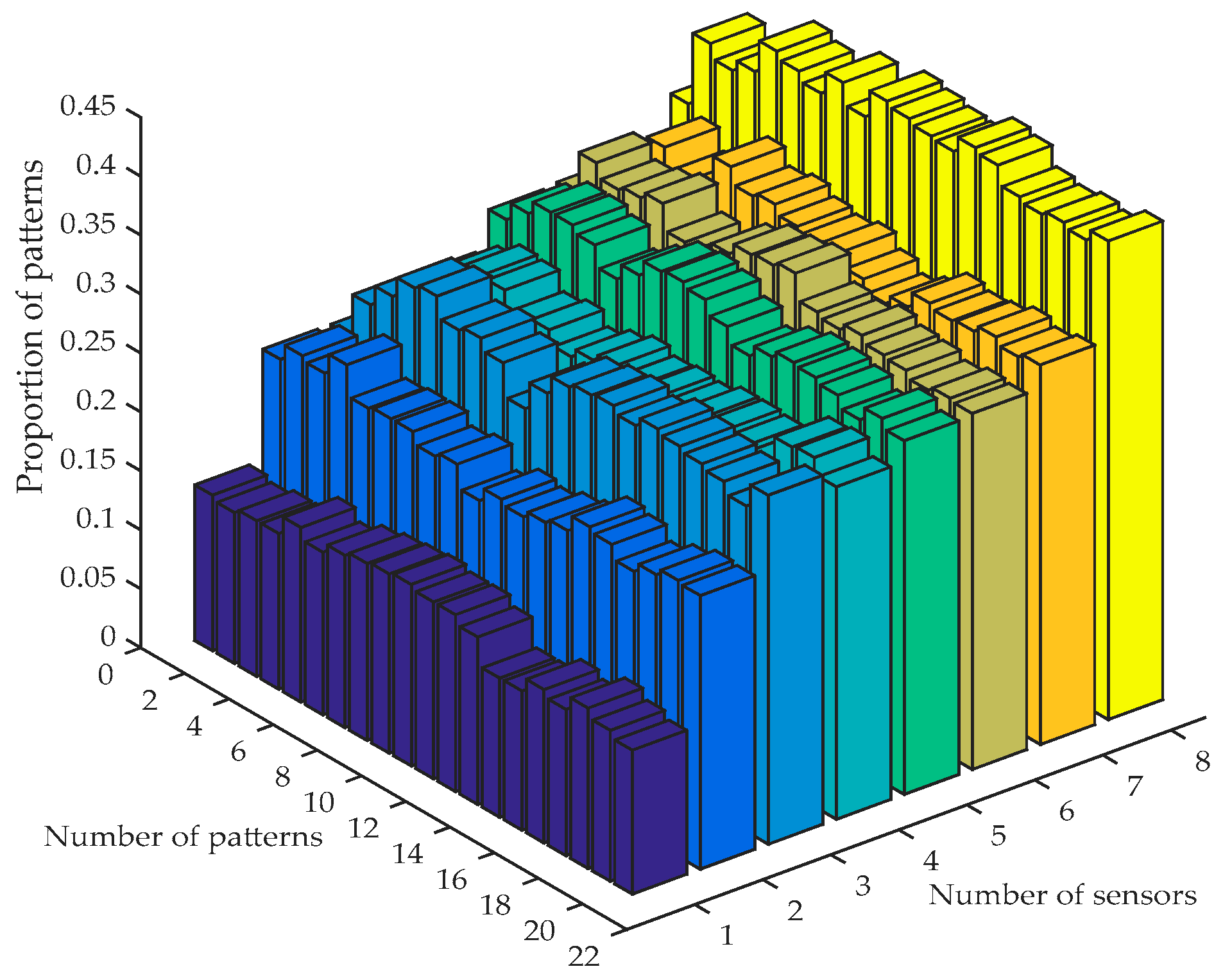
(2) The scenarios with different numbers of sensors and patterns are calculated, the pattern with the stress error of Position A less than 15% is signed, and the property of such a pattern is shown in Figure 3.
(3) There are five optimal combinations including the number of sensors and patterns through Figure 3, which are listed in Table 3. By comparing the five combinations in different error ranges, the fourth scenario is chosen as the optimal parameter for identify the stress of Position A. For all the four subsets of measurement, the optimal parameter for identifying the stress of Position A and Position B can be also obtained and are shown in Table 4 and Table 5. According to the determination process of the number of sensors, recognition parameters in two positions with the whole pattern libraries can be determined, and they are listed in Table 6.
4. Discussion and Analysis
4.1. Comparison of Precision between Distributed and Traditional Concentrated Methods
4.2. Comparison and Analysis of the Results of Distributed and Concentrated Computing
In this section, the proposed distributed method and the traditional concentrated method are compared by considering the noise interferences.
4.2.1. Noise Analysis
Noise level can be defined as the ratio of root-mean-square of noise to that of the time series:
where is the root-mean-square of noise, and is the root-mean-square of the time series.
4.2.2. Noise Interferences on All Observed Sensors
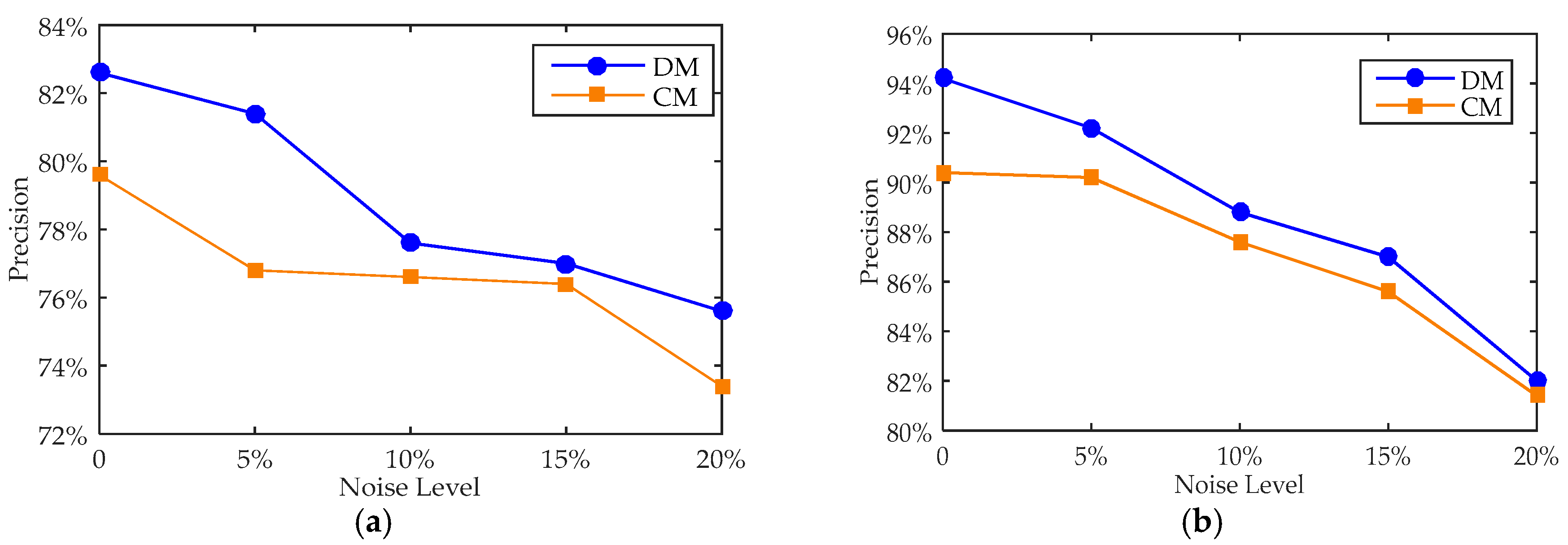
When all the observed measurements are affected by different levels of noise interference, identified stress values of Positions A and B using the proposed distributed method and the traditional concentrated method are calculated. The proportions of the members with a stress error less than 15% are shown in Figure 4.
As shown in Figure 4, compared with the proposed distributed method and traditional concentrated method, the distributed method can perform the stress identification with errors less than the traditional concentrated method; in other words, the proposed distributed method cannot only identify the stress, but also realize the distributed calculation to improve the reliability of the system.
4.2.3. Noise Interferences on a Single Sensor
There are two scenarios: one is that the sensor located on member No. 152 is subjected to noise, which is used to identify the stress of Position A; the other one is that the sensor located on member No. 161 is subjected to noise, which is used to identify the stress of Position B. The error analysis is shown in Figure 5.
As shown in the Figure 5, compared with the not-optimised DM and CM methods, when one sensor is disturbed by noise at various levels, the recognizing precision of DM is improved clearly on both positions. In summary, regardless of how many sensors are disturbed by noise, the DM has more advantages than CM in stress recognition.
5. Stress Recognition Based on Measurements from a Real-World Structure
5.1. Introduction of the Structure
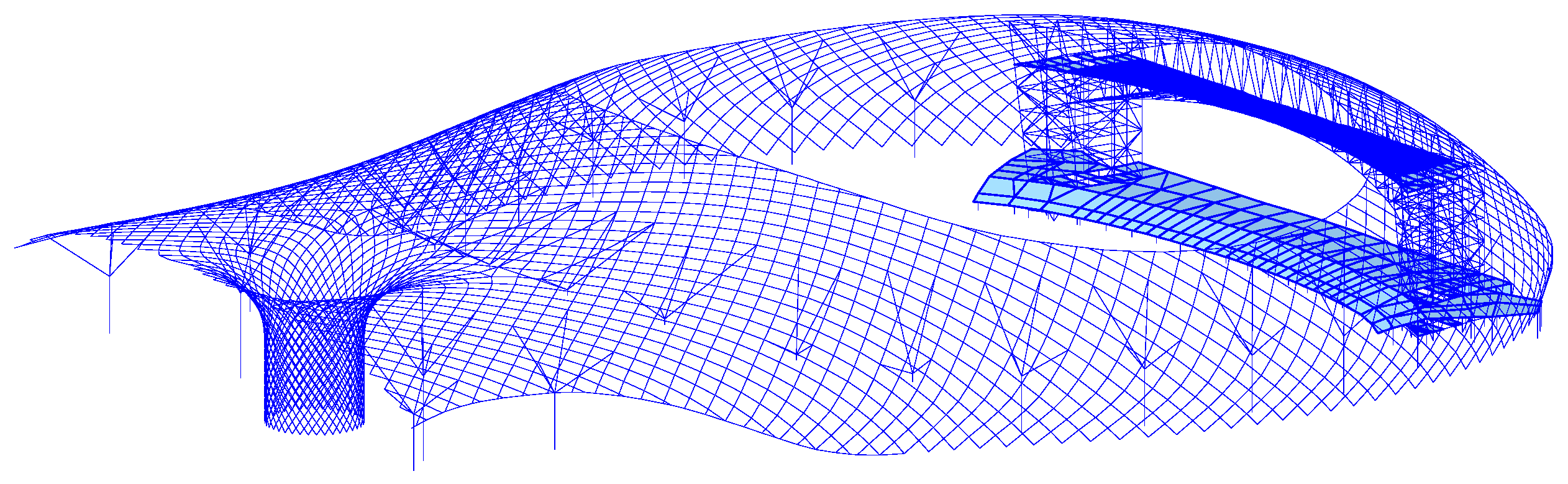
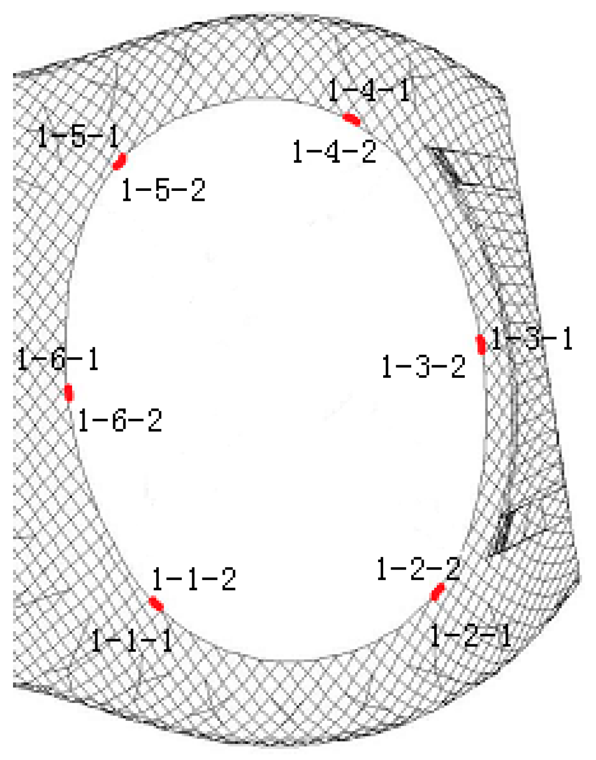
The Shenzhen Bay Stadium was constructed for the 26th Summer World University Games. It consists of a single shell, with double-layer space trusses, and the vertical support system. The finite element model using Midas® is shown in Figure 6. The strain monitoring arranged at the ring members of the front stadium structure are used for stress recognition. In the construction phase, six members are chosen for monitoring, and each of them has one vibrating string strain sensor placed on both sides. The identification number and distribution of the strain sensors are shown in Figure 7 [11,21].
5.2. Pattern Sets
The model can be analysed by instantaneous time-domain analysis in Midas with Earth pulsation, which is simulated by white noise. The amplitudes of accelerations in three orientations X, Y, and Z are 0.1 g, 0.1 g, and 0.15 g, respectively. The frequency range is from 0.5 Hz to 20 Hz and the time range lasts 600 s with a substep of 0.02 s. The stress recognition is that of location 1-2-2 using the other stress measurements.
The stress values extracted from the Midas finite-element method are used to build the pattern library and the testing library, while the stress measurements from the structural health monitoring system of Shenzhen Bay Stadium are used to build the observed library, shown in Table 9.
5.3. Comparison of the Results of Two Stress Recognition Methods
The measurements from the structural health monitoring system are less than those for the simulation example of the shell-like structure, so the comparison of the results is between two scenarios: scenario 1 is the method proposed where the optimal number of sensors and fusion patterns is considered, while scenario 2 is the traditional method where the number of sensors and fusion patterns are fixed. The comparison of the recognition results of the two scenarios is shown in Table 10.
From Table 10, it can be found that the recognition error of Scenario 1 is more stable than that of Scenario 2. The proposed method considering the optimal number of sensors and fusion patterns can be effectively used in real-world projects when the measurements include unknown noise interference. The errors are large; this is mainly because the pattern library is based on the simulation data, where there are errors in the finite-element model. However, the performance of stress identification of this real-world application using the proposed distributed method is better than that of the traditional concentrated method.
6. Conclusions
Stress prediction for the distributed structural health monitoring using existing measurements and pattern recognition is proposed in this paper. The proposed method considered not only the optimal number of sensors, but also the number of fusion patterns. The traditional pattern recognition method is the concentrated method, while the recognition process is divided into several sub-pattern sets, and the calculation is separated. The stress recognition simulation based on the shell-like structure is given, by which the proposed method was proved to be effective, and the precision was influenced by the different noise levels. In addition, the stress measurements collected from the structural health monitoring of the Shenzhen Bay Stadium are used to verify the stability of the proposed method.
Acknowledgments
This research is supported by the National Science Foundation of China (grant No. 51678201, 51308162). Yue Liu edited the formulae and modified the format of the references.
Author Contributions
Wei Lu is in the charge of the whole research work, Jun Teng provided the real-world project and monitoring data, Qiushi Zhou performed the proposed method, and Qiexin Peng translated the paper into English and drew the charts.
Conflicts of Interest
The authors declare no conflicts of interest.
References
- Xiong, W.; Tu, X.; Xiao, R.; Cai, C.S. A stress-development prediction method and its application to stress assessment of existing bridges. Eng. Struct. 2012, 38, 113–122. [Google Scholar] [CrossRef]
- Ye, X.W.; Ni, Y.Q.; Wong, K.Y.; Ko, J.M. Statistical analysis of stress spectra for fatigue life assessment of steel bridges with structural health monitoring data. Eng. Struct. 2012, 45, 166–176. [Google Scholar] [CrossRef]
- Choi, S.W.; Lee, J.; Oh, B.K.; Park, H.S. Analytical models for estimation of the maximum strain of beam structures based on optical fiber Bragg grating sensors. J. Civ. Eng. Manag. 2016, 22, 86–91. [Google Scholar] [CrossRef]
- Zhang, C.D.; Xu, Y.L. Optimal multi-type sensor placement for response and excitation reconstruction. J. Sound Vib. 2016, 360, 112–128. [Google Scholar] [CrossRef]
- Park, J.S.; Oh, B.K.; Choi, S.W.; Park, H.S. Sensor-free stress estimation model for steel beam structures using a motion capture system. IEEE Sens. J. 2016, 16, 2701–2713. [Google Scholar] [CrossRef]
- Fan, X.; Liu, Y. Dynamic extreme stress prediction of bridges based on nonlinear mixed Gaussian particle filtering algorithm and structural health monitoring data. Adv. Mech. Eng. 2016, 8, 1–10. [Google Scholar] [CrossRef]
- Papadimitriou, C.; Fritzen, C.-P.; Kraemer, P.; Ntotsios, E. Fatigue predictions in entire body of metallic structures from a limited number of vibration sensors using Kalman filtering. Struct. Control Health. 2011, 18, 554–573. [Google Scholar] [CrossRef]
- Lourens, E.; Papadimitriou, C.; Gillijns, S.; Reynders, E.; De Roeck, G.; Lombaert, G. Joint input-response estimation for structural systems based on reduced-order models and vibration data from a limited number of sensors. Mech. Syst. Signal Process. 2012, 29, 310–327. [Google Scholar] [CrossRef]
- Hernandez, E.M.; Bernal, D.; Caracoglia, L. On-line monitoring of wind-induced stresses and fatigue damage in instrumented structures. Struct. Control Health. 2013, 20, 1291–1302. [Google Scholar] [CrossRef]
- Erazo, K.; Hernandez, E. A model-based observer for state and stress estimation in structural and mechanical systems: Experimental validation. Mech. Syst. Signal Process. 2014, 43, 141–152. [Google Scholar]
- Lu, W.; Wu, F.; Teng, J.; Zhou, Q. Estimation on structural responses using multi scale measurements. Sci. China Technol. Sci. 2014, 57, 1707–1713. [Google Scholar] [CrossRef]
- Xu, Y.L.; Zhang, X.H.; Zhu, S.Y.; Zhan, S. Multi-type sensor placement and response reconstruction for structural health monitoring of long-span suspension bridges. Sci. Bull. 2016, 61, 313–329. [Google Scholar] [CrossRef]
- Zhang, Z.; Luo, Y. Restoring method for missing data of spatial structural stress monitoring based on correlation. Mech. Syst. Signal Process. 2017, 91, 266–277. [Google Scholar] [CrossRef]
- Smarsly, K.; Law, K.H. Decentralized fault detection and isolation in wireless structural health monitoring systems using analytical redundancy. Adv. Eng. Softw. 2014, 73, 1–10. [Google Scholar] [CrossRef]
- Sim, S.-H.; Juan Francisco, C.-M.; Spencer, B.F., Jr.; Jo, H. Decentralized random decrement technique for efficient data aggregation and system identification in wireless smart sensor networks. Probab. Eng. Mech. 2011, 26, 81–91. [Google Scholar] [CrossRef]
- Lynch, J.R.; Loh, K.J. A Summary Review of wireless sensors and sensor networks for structural health monitoring. Shock Vib. Dig. 2006, 38, 91–128. [Google Scholar] [CrossRef]
- Leng, J.C.; Miao, X.J.; Zhou, G.Q.; Wu, Z.M.; Yan, T.H. Pipeline stress monitoring system based on fiber bragg grating sensors. Control Instrum. Chem. Ind. 2012, 39, 1504–1506. (In Chinese) [Google Scholar]
- Gao, Z.F. Research on Intelligent Information Acquiring and Processing of Health Monitoring for Great Structure. Ph.D. Thesis, Beijing Jiaotong University, Beijing, China, 2010. [Google Scholar]
- Inaudi, D. Development of reusable software components for monitoring data management, visualization and analysis. In Proceedings of the SPIE-Smart Structures and Materials, Smart Systems for Bridges, Structures and Highways, San Diego, CA, USA, 18–21 March 2002; Volume 4696, pp. 10–16. [Google Scholar]
- Lu, W.; Teng, J.; Xu, Y.L.; Su, Z.Q. Identification of damage in dome-like structures using hybrid sensor measurements and artificial neural networks. Smart Mater. Struct. 2013, 22, 105014. [Google Scholar] [CrossRef]
- Teng, J.; Lu, W.; Cui, Y.; Zhang, R.G. Temperature and displacement monitoring to steel roof construction of Shenzhen Bay Stadium. Int. J. Struct. Stab. Dyn. 2016, 16, 1640020. [Google Scholar] [CrossRef]
Figure 1.
The finite-element model. (a) The top view of model; and (b) the side view of model.

Figure 2.
The location of sensors and waited-identification rods. ![Sensors 18 00419 i001]() represents the locations of the displacement sensors,
represents the locations of the displacement sensors, ![Sensors 18 00419 i002]() represents the locations of the strain sensors,
represents the locations of the strain sensors, ![Sensors 18 00419 i003]() represents Position A, and
represents Position A, and ![Sensors 18 00419 i004]() represents Position B.
represents Position B.
 represents the locations of the displacement sensors,
  represents the locations of the strain sensors,
  represents Position A, and
  represents Position B.
Figure 2.
The location of sensors and waited-identification rods. ![Sensors 18 00419 i001]() represents the locations of the displacement sensors,
represents the locations of the displacement sensors, ![Sensors 18 00419 i002]() represents the locations of the strain sensors,
represents the locations of the strain sensors, ![Sensors 18 00419 i003]() represents Position A, and
represents Position A, and ![Sensors 18 00419 i004]() represents Position B.
represents Position B.
represents the locations of the displacement sensors, represents the locations of the strain sensors, represents Position A, and represents Position B.
Figure 3.
Proportion of patterns with stress error of Position A less than 15%.

Figure 4.
The precision comparison between DM and CM. (a) In Position A; and (b) in Position B.

Figure 5.
The precision comparison between DM and CM. (a) In Position A; and (b) in Position B.
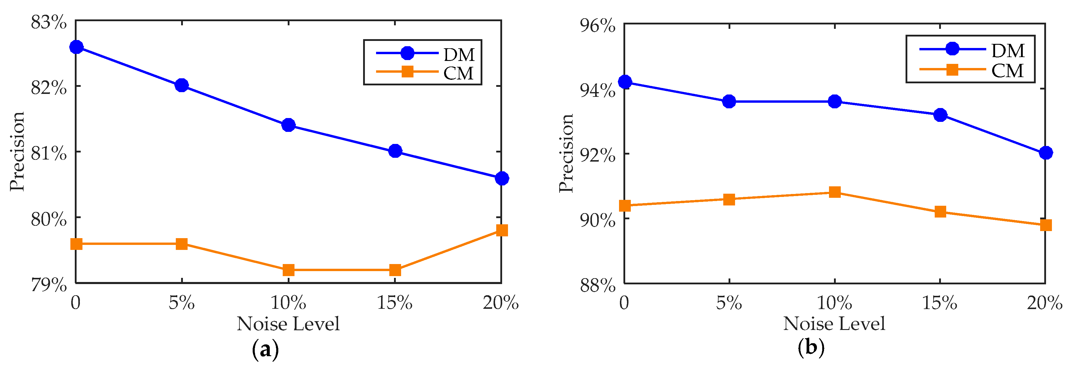
Figure 6.
Finite-element method model of the Shenzhen Bay Stadium.

Figure 7.
Identification numbers and distribution of sensors.


Table 1.
The sensors for each subset of measurement.
| No. of Subset of Measurements | No. of Members or Points | |||||||
|---|---|---|---|---|---|---|---|---|
| 1 (displacements) | 2 | 12 | 13 | 14 | 15 | 16 | 17 | 18 |
| 2 (stresses) | 139 | 161 | 162 | 163 | 164 | 165 | 166 | 168 |
| 3 (stresses) | 129 | 130 | 131 | 132 | 154 | 155 | 156 | 157 |
| 4 (stresses) | 126 | 127 | 128 | 149 | 150 | 151 | 152 | 153 |
Table 2.
Descending rank in the absolute value of correlation.
| Sensor Number | 2 | 12 | 13 | 14 | 15 | 18 | 16 | 17 |
|---|---|---|---|---|---|---|---|---|
| Absolute value of correlation | 0.7657 | 0.3804 | 0.3252 | 0.2892 | 0.2674 | 0.2599 | 0.2560 | 0.2536 |
Table 3.
The number of patterns with the stress identification error less than 15%.
| Parameter (Optimal Number of Sensors and Patterns) | Error Range | |||||
|---|---|---|---|---|---|---|
| <5% | 5–10% | 10–15% | 15–20% | 20–25% | >25% | |
| (8,8) | 64 | 65 | 76 | 60 | 39 | 196 |
| (8,10) | 65 | 75 | 68 | 49 | 55 | 188 |
| (8,11) | 66 | 69 | 70 | 58 | 43 | 194 |
| (8,14) | 66 | 69 | 75 | 58 | 43 | 189 |
| (8,15) | 65 | 70 | 73 | 58 | 41 | 193 |
Table 4.
Parameters of primary agents in Position A.
| Subset of Measurements | Number of Sensors | Number of Fusion Patterns |
|---|---|---|
| No. 1 subset of measurements | 8 | 14 |
| No. 2 subset of measurements | 8 | 12 |
| No. 3 subset of measurements | 8 | 13 |
| No. 4 subset of measurements | 8 | 19 |
Table 5.
Parameters of primary agents in Position B.
| Subset of Measurements | Number of Sensors | Number of Fusion Patterns |
|---|---|---|
| No. 1 subset of measurements | 8 | 18 |
| No. 2 subset of measurements | 7 | 18 |
| No. 3 subset of measurements | 8 | 17 |
| No. 4 subset of measurements | 7 | 17 |
Table 6.
Recognition parameters in two positions with the set of measurements.
| Recognition Positions | Number of Sensors | Number of Fusion Patterns |
|---|---|---|
| A | 11 | 19 |
| B | 6 | 12 |
Table 7.
Precision comparison for two recognizing ways in Position A.
| Recognition Method | Error Range | |||||
|---|---|---|---|---|---|---|
| <5% | 5–10% | 10–15% | 15–20% | 20–25% | >25% | |
| DM | 189 | 140 | 84 | 33 | 23 | 31 |
| CM | 169 | 121 | 97 | 40 | 34 | 39 |
Table 8.
Precision comparison for two recognizing ways in Position B.
| Recognition Method | Error Range | |||||
|---|---|---|---|---|---|---|
| <5% | 5–10% | 10–15% | 15–20% | 20–25% | >25% | |
| DM | 277 | 149 | 45 | 15 | 6 | 8 |
| CM | 227 | 152 | 65 | 29 | 13 | 14 |
Table 9.
Stress measurements in the observed library (MPa).
| Sensor Locations | Year 2012 | Year 2013 | |||||||
|---|---|---|---|---|---|---|---|---|---|
| March 19 | April 23 | May 30 | July 26 | September 7 | October 19 | December 19 | January 23 | March 10 | |
| 1-1-1 | 42.4 | 42 | 40.5 | 39 | 39.1 | 39.5 | 36.6 | 38.9 | 35.2 |
| 1-1-2 | −32.1 | −29.5 | −31.5 | −30.4 | −31.6 | −31.9 | −34.5 | −34.3 | −35 |
| 1-2-1 | −39.1 | −38.1 | −38.1 | −37.9 | −38.1 | −38.1 | −38.1 | −38.1 | −37.9 |
| 1-2-2 | 41.5 | 40.7 | 40.7 | 40.4 | 40.7 | 40.7 | 40.7 | 38.9 | 41.6 |
| 1-3-1 | −60.5 | −67.6 | −61.9 | −63.9 | −63.4 | −67.2 | −67.7 | −67.4 | −66.6 |
| 1-3-2 | −38.9 | −38.2 | −36.4 | −38.2 | −38.2 | −39.1 | −24 | −38.2 | −38.4 |
| 1-4-1 | −14.6 | −14.4 | −14.9 | −14.7 | −16.1 | −16.8 | −20 | −17.9 | −20.1 |
| 1-4-2 | −44.5 | −42.7 | −43.3 | −44.5 | −44.6 | −46.8 | −48.4 | −47.4 | −48 |
| 1-5-1 | −13.9 | −14.3 | −16.4 | −16.3 | −18 | −17.7 | −19.9 | −17.9 | −22.2 |
| 1-5-2 | 15.9 | 17 | 15.1 | 14.7 | 14.7 | 13.2 | 9.1 | 15.2 | 11.5 |
| 1-6-1 | −81.2 | −79.4 | −80.5 | −81.8 | −81.9 | −83.7 | −85 | −82.4 | −82.5 |
| 1-6-2 | −57.3 | −55.8 | −57.6 | −57.1 | −59 | −60.4 | −61.2 | −61.3 | −63.2 |
Table 10.
Comparison of recognition results of two scenarios based on measured data.
| Scenario 1 (MPa) | Scenario 2 (MPa) | Measured Data (MPa) | Error of Scenario 1 | Error of Scenario 2 | Error Difference |
|---|---|---|---|---|---|
| 54.34 | 47.37 | 41.5 | 30.95% | 14.14% | 16.81% |
| 53.01 | 55.21 | 40.7 | 27.71% | 35.66% | −7.95% |
| 54.18 | 55.76 | 40.7 | 33.13% | 37.07% | −3.94% |
| 54.79 | 55.58 | 40.4 | 35.63% | 37.57% | −1.94% |
| 54.88 | 55.79 | 40.7 | 34.84% | 37.08% | −2.24% |
| 54.89 | 55.98 | 40.7 | 34.87% | 37.50% | −2.63% |
| 43.22 | 19.01 | 40.7 | 6.20% | 53.27% | −47.07% |
| 42.99 | 48.21 | 38.9 | 10.51% | 23.94% | −13.43% |
| 48.31 | 51.07 | 41.6 | 16.14% | 22.77% | −6.63% |
© 2018 by the authors. Licensee MDPI, Basel, Switzerland. This article is an open access article distributed under the terms and conditions of the Creative Commons Attribution (CC BY) license (http://creativecommons.org/licenses/by/4.0/).
Share and Cite
MDPI and ACS Style
Lu, W.; Teng, J.; Zhou, Q.; Peng, Q. Stress Prediction for Distributed Structural Health Monitoring Using Existing Measurements and Pattern Recognition. Sensors 2018, 18, 419. https://doi.org/10.3390/s18020419
AMA Style
Lu W, Teng J, Zhou Q, Peng Q. Stress Prediction for Distributed Structural Health Monitoring Using Existing Measurements and Pattern Recognition. Sensors. 2018; 18(2):419. https://doi.org/10.3390/s18020419
Chicago/Turabian StyleLu, Wei, Jun Teng, Qiushi Zhou, and Qiexin Peng. 2018. "Stress Prediction for Distributed Structural Health Monitoring Using Existing Measurements and Pattern Recognition" Sensors 18, no. 2: 419. https://doi.org/10.3390/s18020419
Note that from the first issue of 2016, this journal uses article numbers instead of page numbers. See further details here.