Drive-By Bridge Frequency Identification under Operational Roadway Speeds Employing Frequency Independent Underdamped Pinning Stochastic Resonance (FI-UPSR)


Abstract
:1. Introduction
2. Frequency Independent Underdamped Pinning Stochastic Resonance (FI-UPSR)
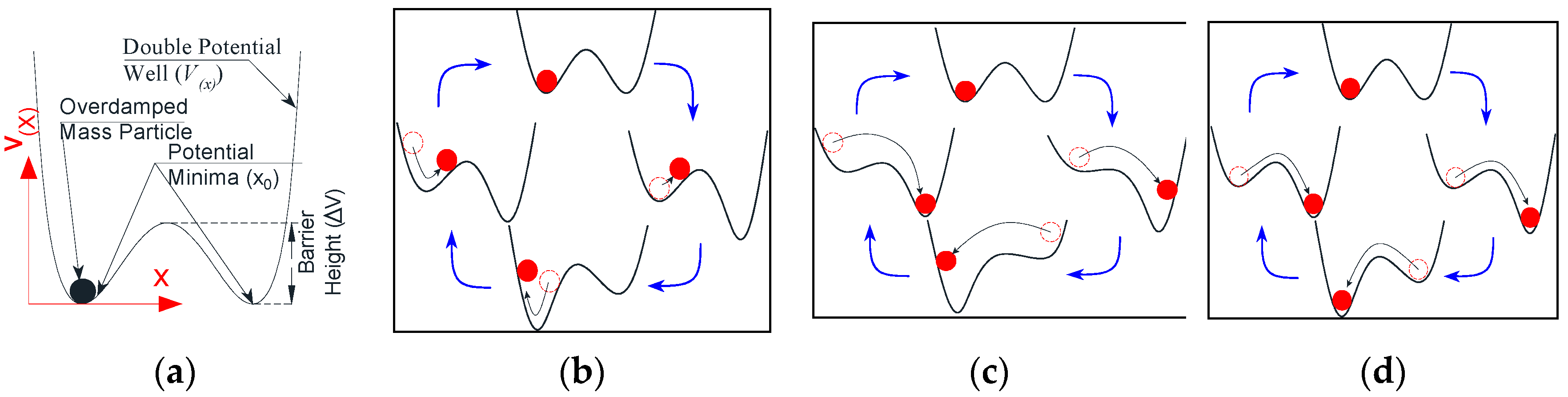
2.1. Background to Underdamped Pinning Stochastic Resonance (UPSR)
2.2. Frequency Independent Underdamped Pinning Stochastic Resonance FI-UPSR
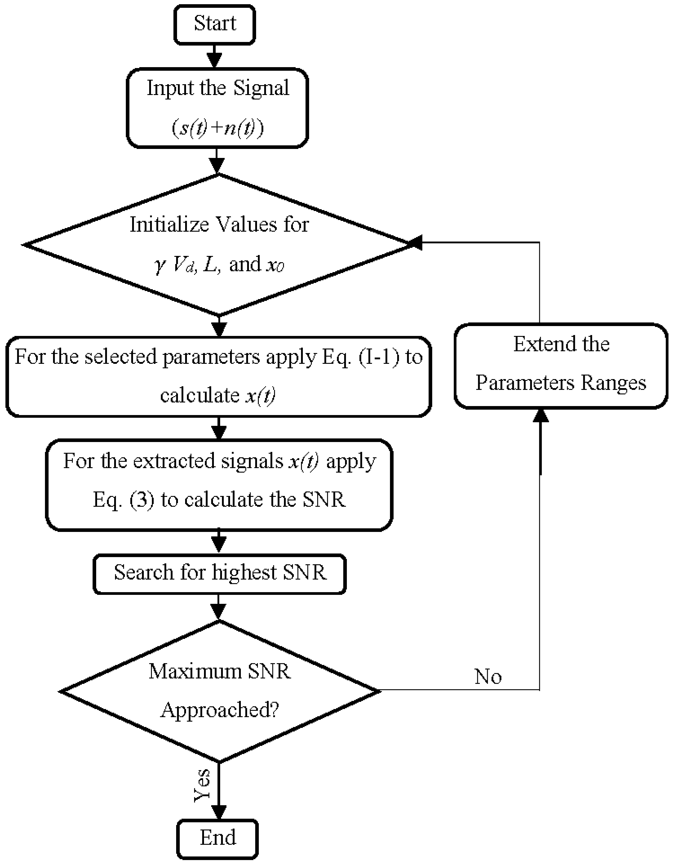
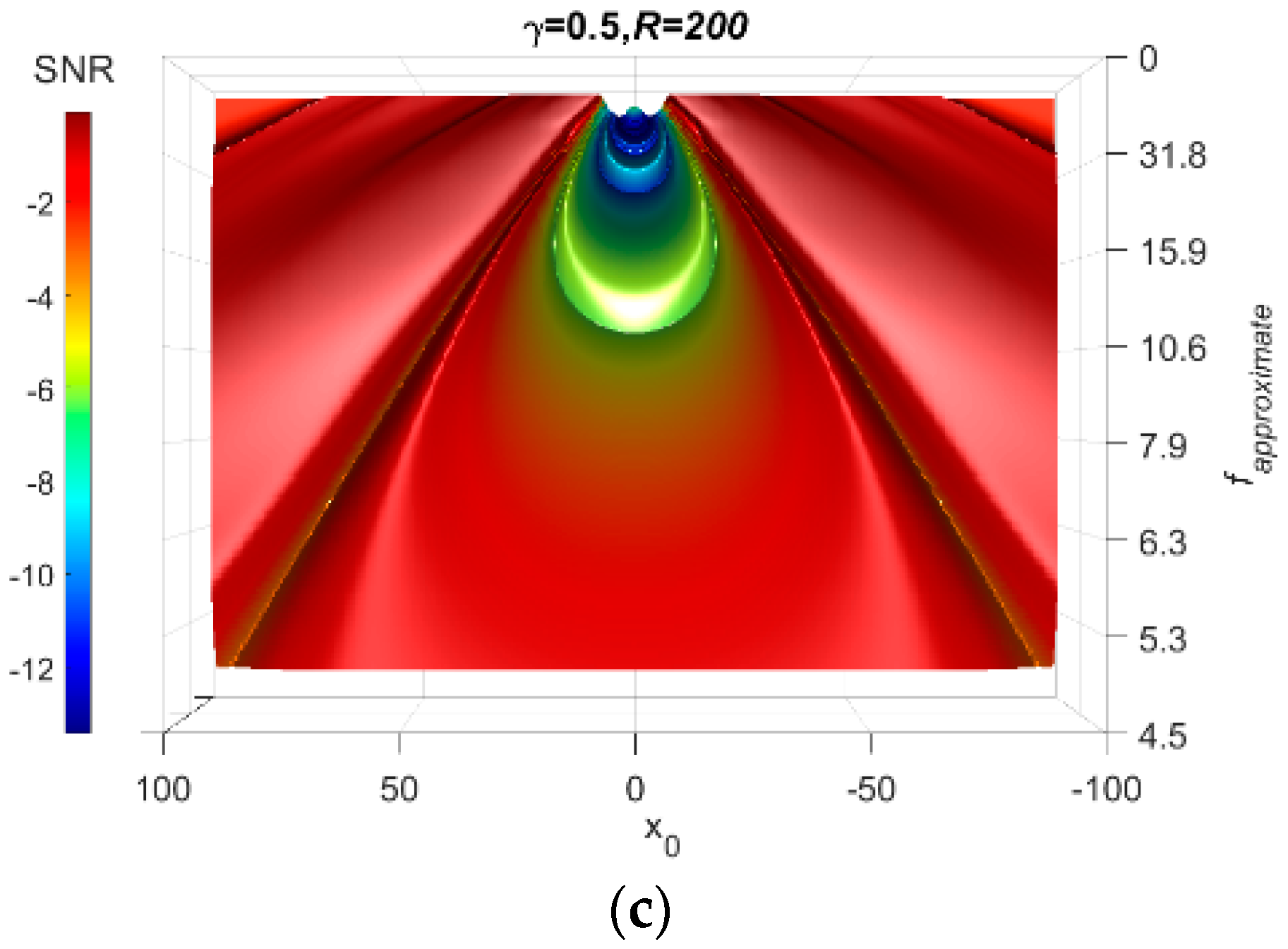
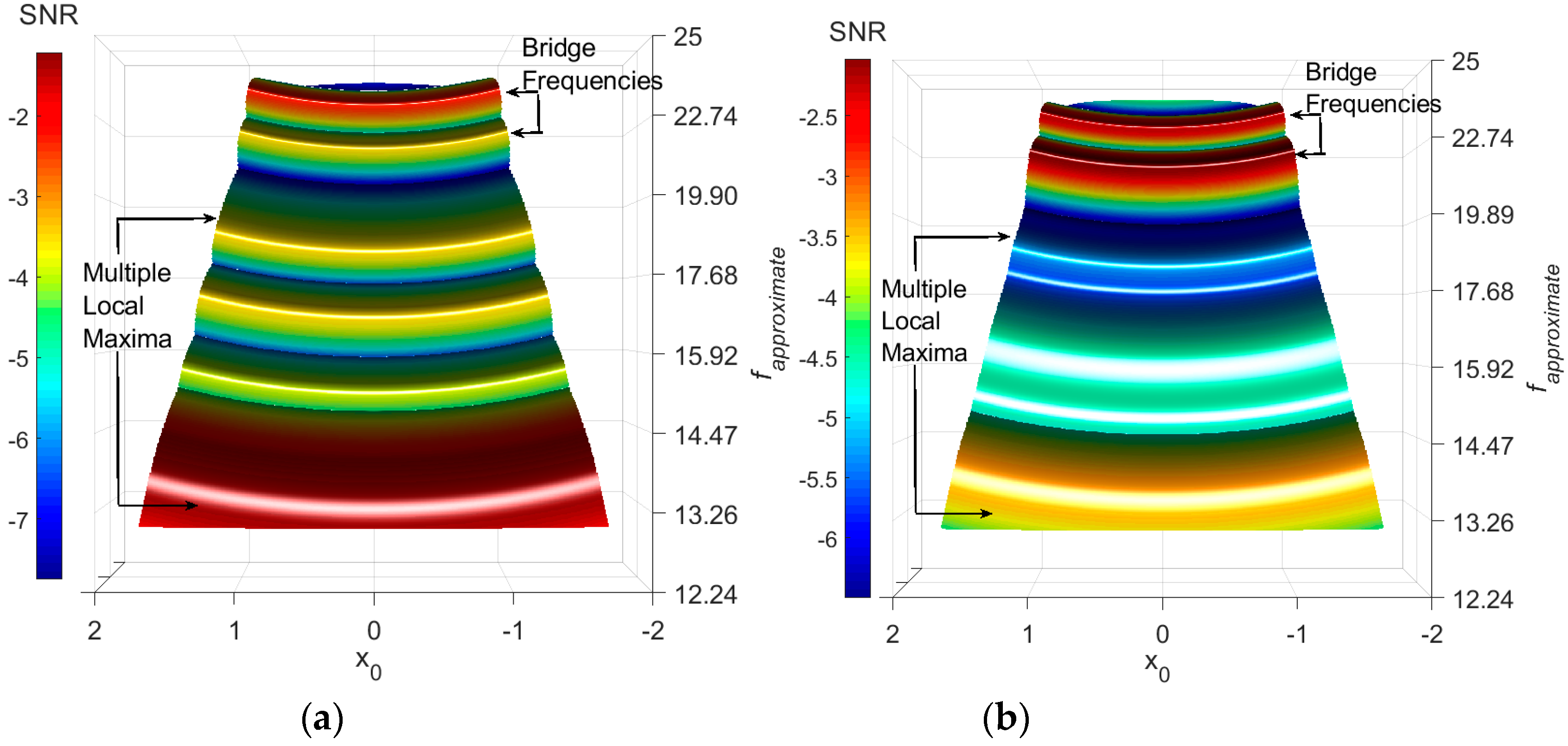
2.3. Investigating the FI-UPSR Approach
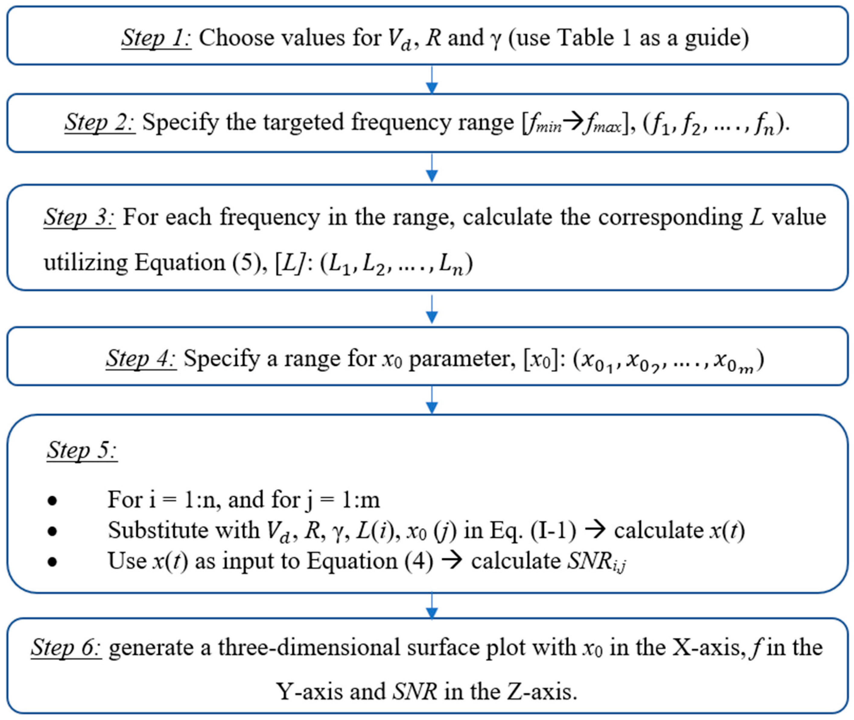
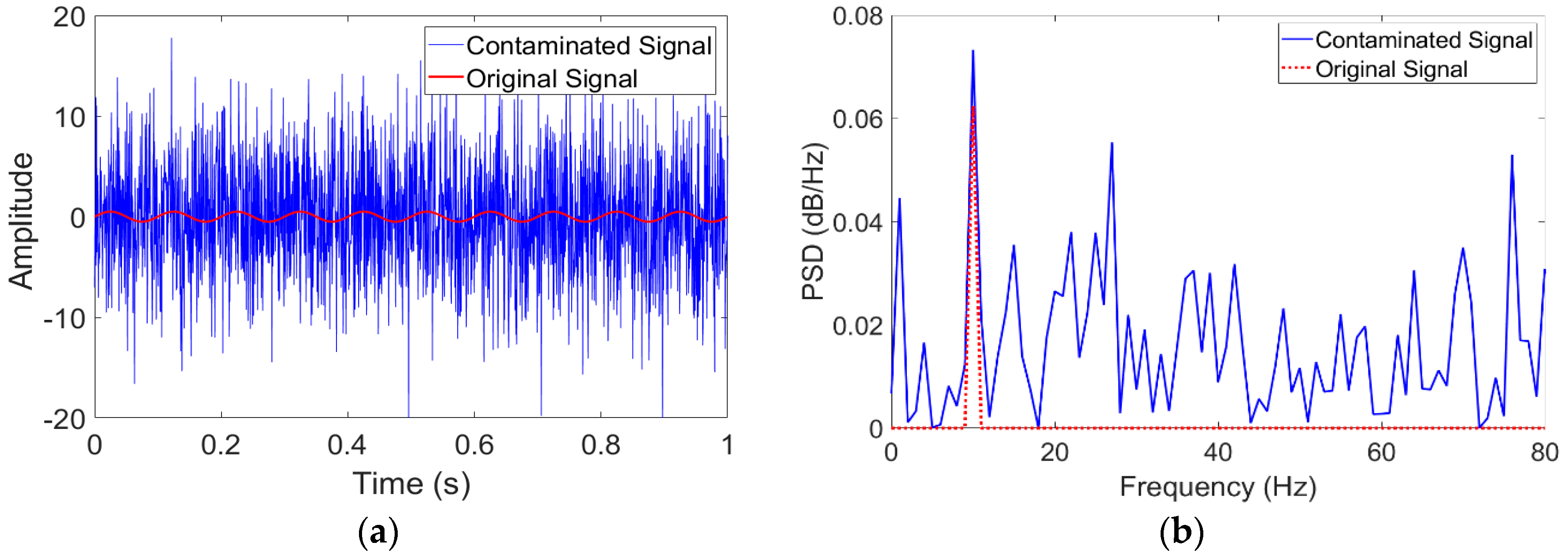
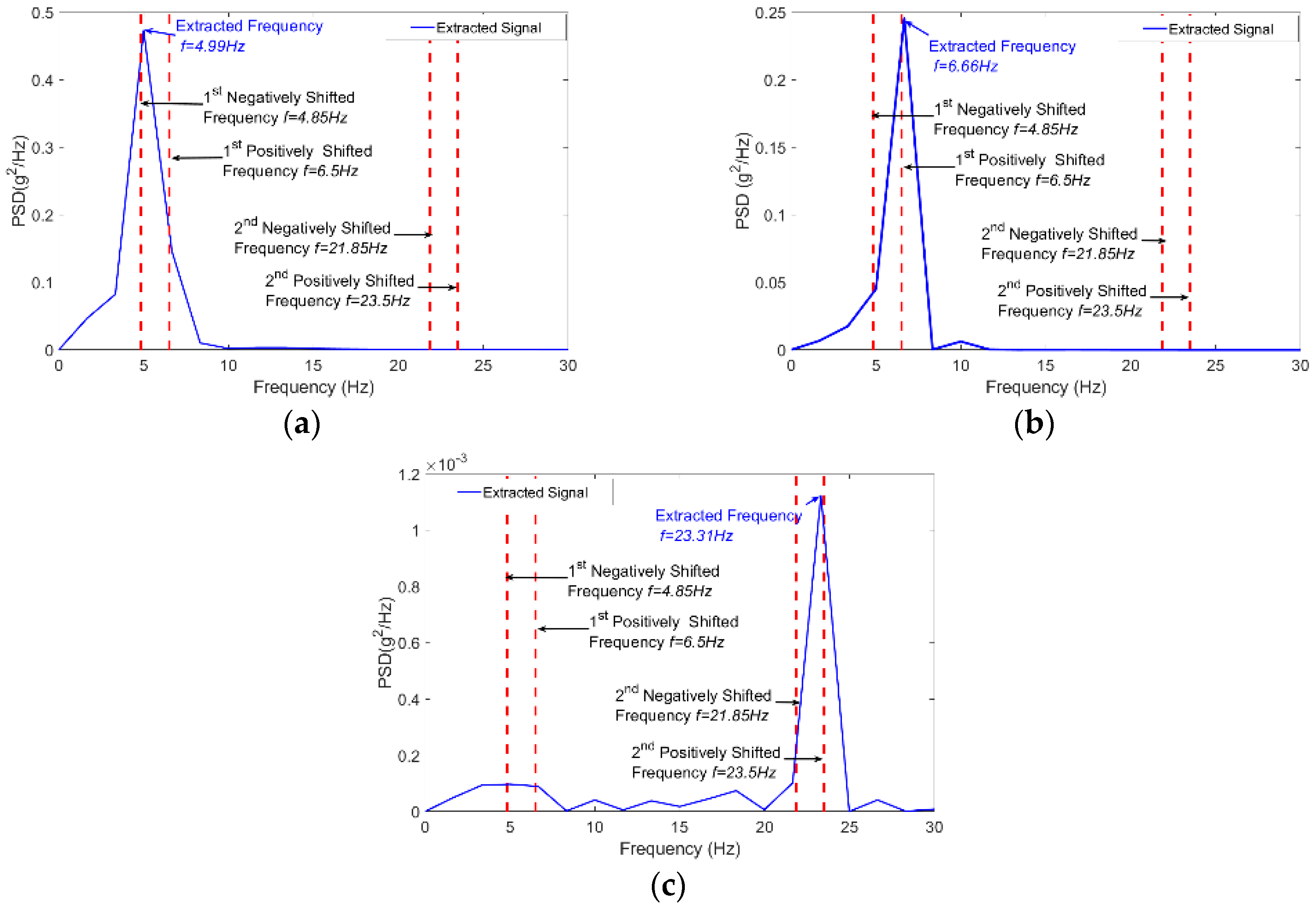
3. Extract Bridge Frequency from a Fast Passing Vehicle Signal Using FI-UPSR
4. FI-UPSR Fidelity for Full Scale Field Test Data
5. Conclusions
Author Contributions
Funding
Acknowledgments
Conflicts of Interest
Appendix A
Appendix B
References
- Davis, S.; DeGood, K.; Donohue, N.; Goldberg, D. The Fix We’re in for: The State of Our Nation’s Busiest Bridges; Transportation for America: Washington, DC, USA, 2013. [Google Scholar]
- Federal Highway Administration. 2015 Status of the Nation’s Highways, Bridges, and Transit Conditions & Performance Report to Congress; 016093706X; Federal Highway Administration: Washington, DC, USA, 2017.
- Stanbridge, A.; Khan, A.; Ewins, D. Fault identification in vibrating structures using a scanning laser doppler vibrometer. In Proceedings of the International Workshop on Structural Health Monitoring, Stanford, CA, USA, 12–14 September 2017; pp. 56–65. [Google Scholar]
- Zhang, L.; Zhao, H.; OBrien, E.J.; Shao, X. Virtual Monitoring of orthotropic steel deck using bridge weigh-in-motion algorithm: Case study. Struct. Health Monit. 2018. [Google Scholar] [CrossRef]
- Zang, C.; Friswell, M.I.; Imregun, M. Structural Damage Detection using Independent Component Analysis. Struct. Health Monit. 2004, 3, 69–83. [Google Scholar] [CrossRef]
- Keenahan, J.; Obrien, E.J.; McGetrick, P.J.; Gonzalez, A. The use of a dynamic truck–trailer drive-by system to monitor bridge damping. Struct. Health Monit. 2013, 13, 143–157. [Google Scholar] [CrossRef] [Green Version]
- Tong, G.; Aiqun, L.; Jianhui, L. Fatigue Life Prediction of Welded Joints in Orthotropic Steel Decks Considering Temperature Effect and Increasing Traffic Flow. Struct. Health Monit. 2008, 7, 189–202. [Google Scholar] [CrossRef]
- Fan, W.; Qiao, P. Vibration-based damage identification methods: A review and comparative study. Struct. Health Monit. 2011, 10, 83–111. [Google Scholar] [CrossRef]
- Carden, E.P.; Fanning, P. Vibration based condition monitoring: A review. Struct. Health Monit. 2004, 3, 355–377. [Google Scholar] [CrossRef]
- Chang, P.C.; Flatau, A.; Liu, S. Health monitoring of civil infrastructure. Struct. Health Monit. 2003, 2, 257–267. [Google Scholar] [CrossRef]
- Yang, Y.; Chang, K. Extracting the bridge frequencies indirectly from a passing vehicle: Parametric study. Eng. Struct. 2009, 31, 2448–2459. [Google Scholar] [CrossRef]
- Malekjafarian, A.; McGetrick, P.J.; OBrien, E.J. A Review of Indirect Bridge Monitoring Using Passing Vehicles. Shock Vib. 2015, 2015, 286139. [Google Scholar] [CrossRef] [Green Version]
- Ramadan, O.; Sisiopiku, V. Impact of Bottleneck Merge Control Strategies on Freeway Level of Service. Transp. Res. Procedia 2016, 15, 583–593. [Google Scholar] [CrossRef]
- Ramadan, O.E.; Sisiopiku, V.P. Bottleneck Merge Control Strategies for Work Zones: Available Options and Current Practices. Open J. Civ. Eng. 2015, 5, 428–436. [Google Scholar] [CrossRef]
- Ramadan, O.E.; Sisiopiku, V.P. Evaluation of merge control strategies at interstate work zones under peak and off-peak traffic conditions. J. Transp. Technol. 2016, 6, 118–130. [Google Scholar] [CrossRef]
- Kim, C.W.; Kawatani, M. Challenge for a drive-by bridge inspection. In Proceedings of the 10th International Conferenceon Structural Safety and Reliability, ICOSSAR, Osaka, Japan, 13–17 September 2009; pp. 758–765. [Google Scholar]
- Yang, Y.; Lin, C. Vehicle–bridge interaction dynamics and potential applications. J. Sound Vib. 2005, 284, 205–226. [Google Scholar] [CrossRef]
- Yang, Y.-B.; Lin, C.; Yau, J. Extracting bridge frequencies from the dynamic response of a passing vehicle. J. Sound Vib. 2004, 272, 471–493. [Google Scholar] [CrossRef]
- McGetrick, P.J.; González, A.; OBrien, E.J. Theoretical investigation of the use of a moving vehicle to identify bridge dynamic parameters. Insight Non-Destr. Test. Cond. Monit. 2009, 51, 433–438. [Google Scholar] [CrossRef] [Green Version]
- Toshinami, T.; Kawatani, M.; Kim, C. Feasibility investigation for identifying bridge’s fundamental frequencies from vehicle vibrations. In Proceedings of the Fifth International IABMAS Conference on Bridge Maintenance, Safety, Management and Life-Cycle Optimization, Philadelphia, PA, USA, 11–15 July 2010; p. 108. [Google Scholar]
- Keenahan, J.; McGetrick, P.; O’Brien, E.J.; Gonzalez, A. Using instrumented vehicles to detect damage in bridges. In Proceedings of the 15th International Conference on Experimental Mechanics, Porto, Portugal, 22–27 July 2012. Paper No. 2934. [Google Scholar]
- O’Brien, E.J.; Keenahan, J.; McGetrick, P.; González, A. Using Instrumented Vehicles to Detect Damage in Bridges. In Proceedings of the BCRI 12-Bridge and Concrete Research in Ireland, Dublin, Ireland, 6–7 September 2012. [Google Scholar]
- González, A.; OBrien, E.J.; McGetrick, P.J. Detection of bridge dynamic parameters using an instrumented vehicle. In Proceedings of the 5th World Conference on Structural Control and Monitoring, Tokyo, Japan, 12–14 July 2010. [Google Scholar]
- McGetrick, P.J.; González, A.; O’Brien, E.J. Monitoring bridge dynamic behaviour using an instrumented two axle vehicle. In Proceedings of the Bridge and Infrastructure Research in Ireland 2010 (BRI 10), Cork, Ireland, 2–3 September 2010. [Google Scholar]
- ElHattab, A.; Uddin, N.; OBrien, E. Drive-by bridge damage detection using non-specialized instrumented vehicle. Bridge Struct. 2017, 12, 73–84. [Google Scholar] [CrossRef]
- El-hattab, A.; Uddin, N.; OBrien, E. Drive-By Bridge Damage Detection Using Apparent Profile. In Proceedings of the First International Conference on Advances in Civil Infrastructure and Construction Materials (CISM), Dhaka, Bangladesh, 14–15 December 2015; pp. 33–45. [Google Scholar]
- Lin, C.; Yang, Y. Use of a passing vehicle to scan the fundamental bridge frequencies: An experimental verification. Eng. Struct. 2005, 27, 1865–1878. [Google Scholar] [CrossRef]
- Oshima, Y.; Yamaguchi, T.; Kobayashi, Y.; Sugiura, K. Eigenfrequency estimation for bridges using the response of a passing vehicle with excitation system. In Proceedings of the Fourth International Conference on Bridge Maintenance, Safety and Management, Seoul, Korea, 13–17 July 2008; pp. 3030–3037. [Google Scholar]
- Benzi, R.; Sutera, A.; Vulpiani, A. The mechanism of stochastic resonance. J. Phys. A Math. Gen. 1981, 14, L453. [Google Scholar] [CrossRef]
- Gammaitoni, L.; Hänggi, P.; Jung, P.; Marchesoni, F. Stochastic resonance. Rev. Mod. Phys. 1998, 70, 223. [Google Scholar] [CrossRef]
- Levin, J.E.; Miller, J.P. Broadband neural encoding in the cricket cereal sensory system enhanced by stochastic resonance. Nature 1996, 380, 165–168. [Google Scholar] [CrossRef] [PubMed]
- Chapeau-Blondeau, F. Stochastic resonance and optimal detection of pulse trains by threshold devices. Digit. Signal Process. 1999, 9, 162–177. [Google Scholar] [CrossRef]
- Jung, P.; Hänggi, P. Amplification of small signals via stochastic resonance. Phys. Rev. A 1991, 44, 8032–8042. [Google Scholar] [CrossRef] [PubMed]
- He, H.-L.; Wang, T.-Y.; Leng, Y.-G.; Zhang, Y.; Li, Q. Study on non-linear filter characteristic and engineering application of cascaded bistable stochastic resonance system. Mech. Syst. Signal Process. 2007, 21, 2740–2749. [Google Scholar] [CrossRef]
- He, Q.; Wang, J. Effects of multiscale noise tuning on stochastic resonance for weak signal detection. Digit. Signal Process. 2012, 22, 614–621. [Google Scholar] [CrossRef]
- Han, D.; An, S.; Shi, P. Multi-frequency weak signal detection based on wavelet transform and parameter compensation band-pass multi-stable stochastic resonance. Mech. Syst. Signal Process. 2016, 70, 995–1010. [Google Scholar] [CrossRef]
- Chen, Z.; Liu, J.; Zhan, C.; He, J.; Wang, W. Reconstructed Order Analysis-Based Vibration Monitoring under Variable Rotation Speed by Using Multiple Blade Tip-Timing Sensors. Sensors 2018, 18, 3235. [Google Scholar] [CrossRef] [PubMed]
- Lai, Z.-H.; Leng, Y.-G. Generalized parameter-adjusted stochastic resonance of duffing oscillator and its application to weak-signal detection. Sensors 2015, 15, 21327–21349. [Google Scholar] [CrossRef] [PubMed]
- Huang, Q.; Liu, J.; Li, H. A modified adaptive stochastic resonance for detecting faint signal in sensors. Sensors 2007, 7, 157–165. [Google Scholar] [CrossRef]
- Lu, S.; He, Q.; Zhang, H.; Zhang, S.; Kong, F. Note: Signal amplification and filtering with a tristable stochastic resonance cantilever. Rev. Sci. Instrum. 2013, 84, 026110. [Google Scholar] [CrossRef] [PubMed]
- Pollak, E.; Talkner, P. Kramers turnover theory for a triple well potential. Acta Phys. Pol. B 2001, 32, 361. [Google Scholar]
- Zhang, H.; Kong, F.; Lu, S.; He, Q. A Tri-Stable stochastic resonance model and its applying in detection of weak signal. In Proceedings of the 2013 Fourth International Conference on Intelligent Control and Information Processing (ICICIP), Beijing, China, 9–11 June 2013; pp. 199–204. [Google Scholar]
- Li, J.; Chen, X.; He, Z. Multi-stable stochastic resonance and its application research on mechanical fault diagnosis. J. Sound Vib. 2013, 332, 5999–6015. [Google Scholar] [CrossRef]
- Alfonsi, L.; Gammaitoni, L.; Santucci, S.; Bulsara, A. Intrawell stochastic resonance versus interwell stochastic resonance in underdamped bistable systems. Phys. Rev. E 2000, 62, 299–302. [Google Scholar] [CrossRef]
- Almog, R.; Zaitsev, S.; Shtempluck, O.; Buks, E. Signal amplification in a nanomechanical Duffing resonator via stochastic resonance. Appl. Phys. Lett. 2007, 90, 013508. [Google Scholar] [CrossRef] [Green Version]
- Kang, Y.-M.; Xu, J.-X.; Xie, Y. Observing stochastic resonance in an underdamped bistable Duffing oscillator by the method of moments. Phys. Rev. E 2003, 68, 036123. [Google Scholar] [CrossRef] [PubMed]
- Ray, R.; Sengupta, S. Stochastic resonance in underdamped, bistable systems. Phys. Lett. A 2006, 353, 364–371. [Google Scholar] [CrossRef] [Green Version]
- Xu, Y.; Wu, J.; Zhang, H.-Q.; Ma, S.-J. Stochastic resonance phenomenon in an underdamped bistable system driven by weak asymmetric dichotomous noise. Nonlinear Dyn. 2012, 70, 531–539. [Google Scholar] [CrossRef]
- Wang, J.; He, Q.; Kong, F. Adaptive multiscale noise tuning stochastic resonance for health diagnosis of rolling element bearings. IEEE Trans. Instrum. Meas. 2015, 64, 564–577. [Google Scholar] [CrossRef]
- Zhang, H.; He, Q.; Kong, F. Stochastic resonance in an underdamped system with pinning potential for weak signal detection. Sensors 2015, 15, 21169–21195. [Google Scholar] [CrossRef] [PubMed]
- Rogowitz, B.E.; Treinish, L.A. Why Should Engineers and Scientists Be Worried About Color? 1996. Available online: http://www.research.ibm.com/people/l/lloydt/color/color.htm (accessed on 18 March 2010).
- Light, A.; Bartlein, P.J. The end of the rainbow? Color schemes for improved data graphics. Eos Trans. Am. Geophys. Union 2004, 85, 385–391. [Google Scholar] [CrossRef]
- Elhattab, A.; Uddin, N.; OBrien, E. Drive-by bridge damage monitoring using Bridge Displacement Profile Difference. J. Civ. Struct. Health Monit. 2016, 6, 839–850. [Google Scholar] [CrossRef]
- ISO-8608. Mechanical Vibration-Road Surface Profiles-Reporting of Measured Data; International Organization for Standardization (ISO): Geneva, Switzerland, 1995. [Google Scholar]
- Wang, Y.; Uddin, N.; Jacobs, L.J.; Kim, J.-Y. Field Validation of a Drive-By Bridge Inspection System with Wireless BWIM+ NDE Devices; National Center for Transportation Systems Productivity and Management: Atlanta, GA, USA, 2016. [Google Scholar]
- Dong, X.; Zhu, D.; Wang, Y.; Lynch, J.P.; Swartz, R.A. Design and validation of acceleration measurement using the Martlet wireless sensing system. In Proceedings of the ASME 2014 Conference on Smart Materials, Adaptive Structures and Intelligent Systems, Newport, RI, USA, 8–10 September 2014; p. V001T005A006. [Google Scholar]
- Yang, Y.; Cheng, M.; Chang, K. Frequency variation in vehicle–bridge interaction systems. Int. J. Struct. Stab. Dyn. 2013, 13, 1350019. [Google Scholar] [CrossRef]


| Vd | R | γ |
|---|---|---|
| ≥100 | 25–75 | 0.1–0.7 |
| For dt = 0.01–0.0005 |
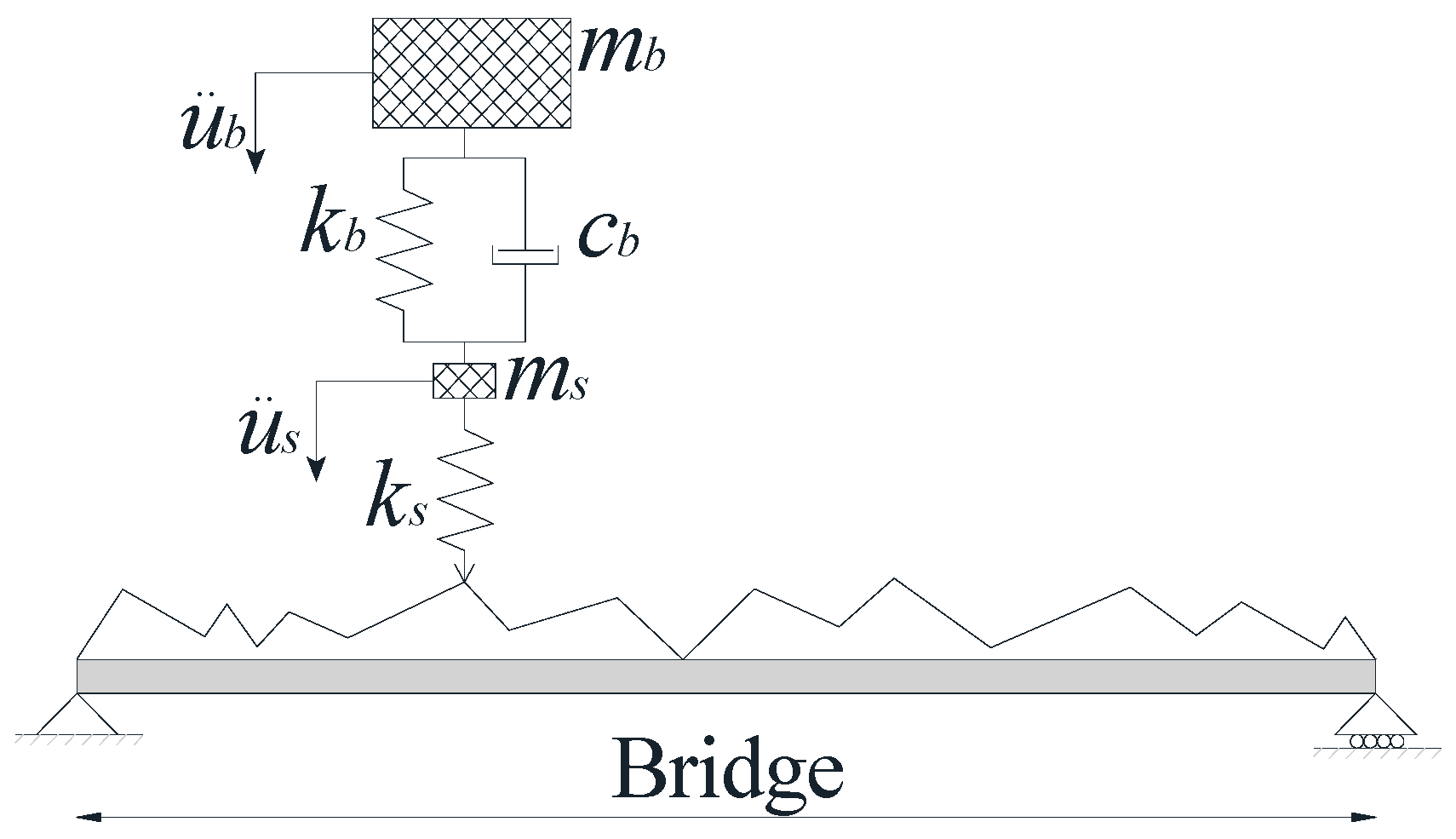
| Property | Unit | Symbol | Value |
|---|---|---|---|
| Body Mass | kg | mb | 16,600 |
| Axle Mass | kg | ms | 700 |
| Body Stiffness | N/m | kb | 2 × 10⁴ |
| Body Damping | N.s/m | cb | 10 × 103 |
| Suspension Stiffness | N/m | ks | 2.75 × 10⁵ |
| Body Bounce Frequency | Hz | fbounce | 0.169 |
| Axle Hop Frequency | Hz | faxle | 3.27 |
| Property | Unit | Value |
|---|---|---|
| Length | m | 15 |
| Mass Per Unit Length | kg/m | 28,125 |
| Elastic Modulus | MPa | 35,000 |
| Second Moment of Area | m4 | 0.5273 |
| 1st Frequency | Hz | 5.67 |
| 2nd Frequency | Hz | 22.69 |
| 3rd Frequency | Hz | 51.05 |
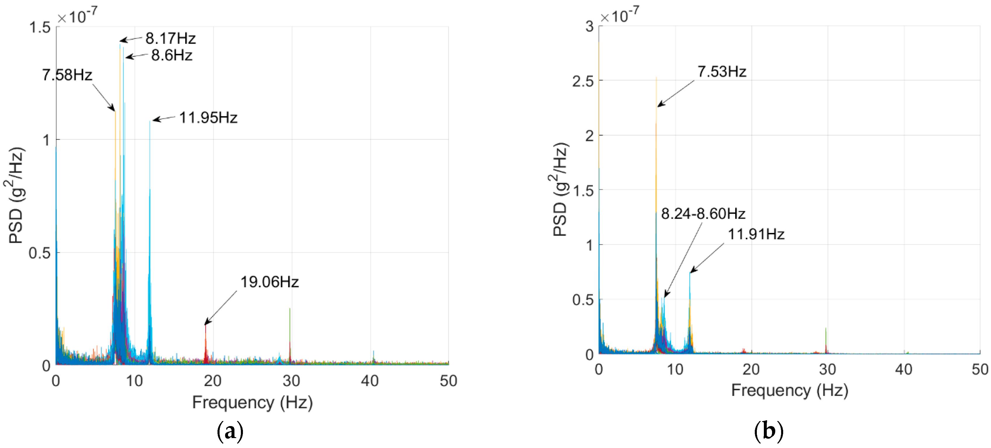
| 1st | 2nd | 3rd | 4th |
|---|---|---|---|
| 7.56 | 8.4 | 11.93 | 19.04 |
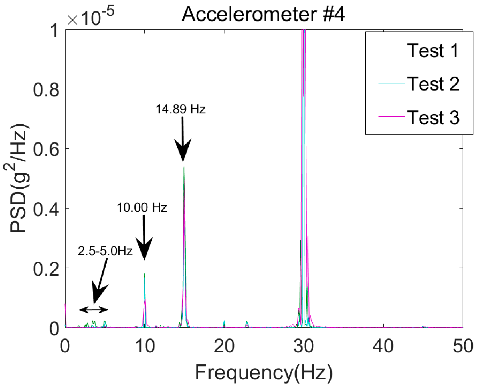
| Test 1 | Test 2 | Test 3 |
|---|---|---|
| 37 | 51 | 53 |
© 2018 by the authors. Licensee MDPI, Basel, Switzerland. This article is an open access article distributed under the terms and conditions of the Creative Commons Attribution (CC BY) license (http://creativecommons.org/licenses/by/4.0/).
Share and Cite
Elhattab, A.; Uddin, N.; OBrien, E. Drive-By Bridge Frequency Identification under Operational Roadway Speeds Employing Frequency Independent Underdamped Pinning Stochastic Resonance (FI-UPSR). Sensors 2018, 18, 4207. https://doi.org/10.3390/s18124207
Elhattab A, Uddin N, OBrien E. Drive-By Bridge Frequency Identification under Operational Roadway Speeds Employing Frequency Independent Underdamped Pinning Stochastic Resonance (FI-UPSR). Sensors. 2018; 18(12):4207. https://doi.org/10.3390/s18124207
Chicago/Turabian StyleElhattab, Ahmed, Nasim Uddin, and Eugene OBrien. 2018. "Drive-By Bridge Frequency Identification under Operational Roadway Speeds Employing Frequency Independent Underdamped Pinning Stochastic Resonance (FI-UPSR)" Sensors 18, no. 12: 4207. https://doi.org/10.3390/s18124207