A Unified Deep-Learning Model for Classifying the Cross-Country Skiing Techniques Using Wearable Gyroscope Sensors

 ,
,
Abstract
:1. Introduction
1.1. Problem Definition
1.2. Literature Review and Proposed Work
2. Materials and Methods
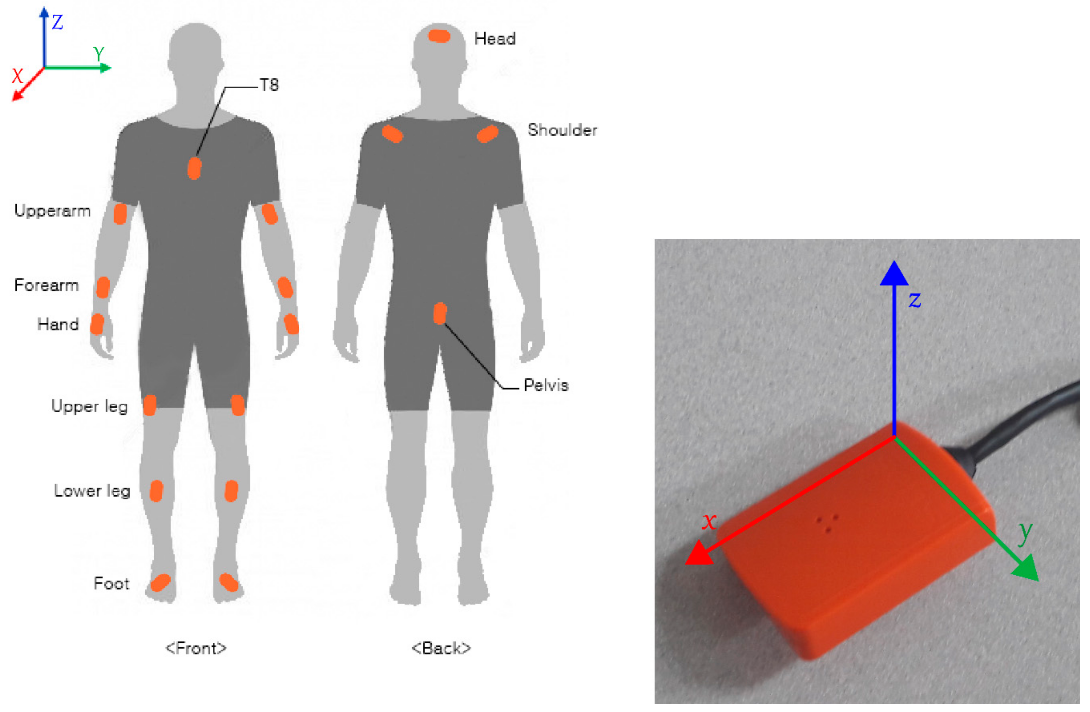
2.1. Inertial Sensors, Synchronization and Calibration
2.2. Data Acquisition
2.2.1. Training and Validation Data Acquisition
2.2.2. Test Data Acquisition
- (i)
- Test set 1: In the first type of test data, the subject is allowed to perform only one of the techniques of one of the XC-skiing styles on the flat course. As there are 4 classical and 4 skating techniques, this test set consists of 8 files.
- (ii)
- Test set 2: In the second type of test data, the subject performs all the skating style techniques on a natural course simultaneously. The subject is allowed to make transitions between the various skating techniques similar to what would be performed during a competition. One data file is obtained in this manner.
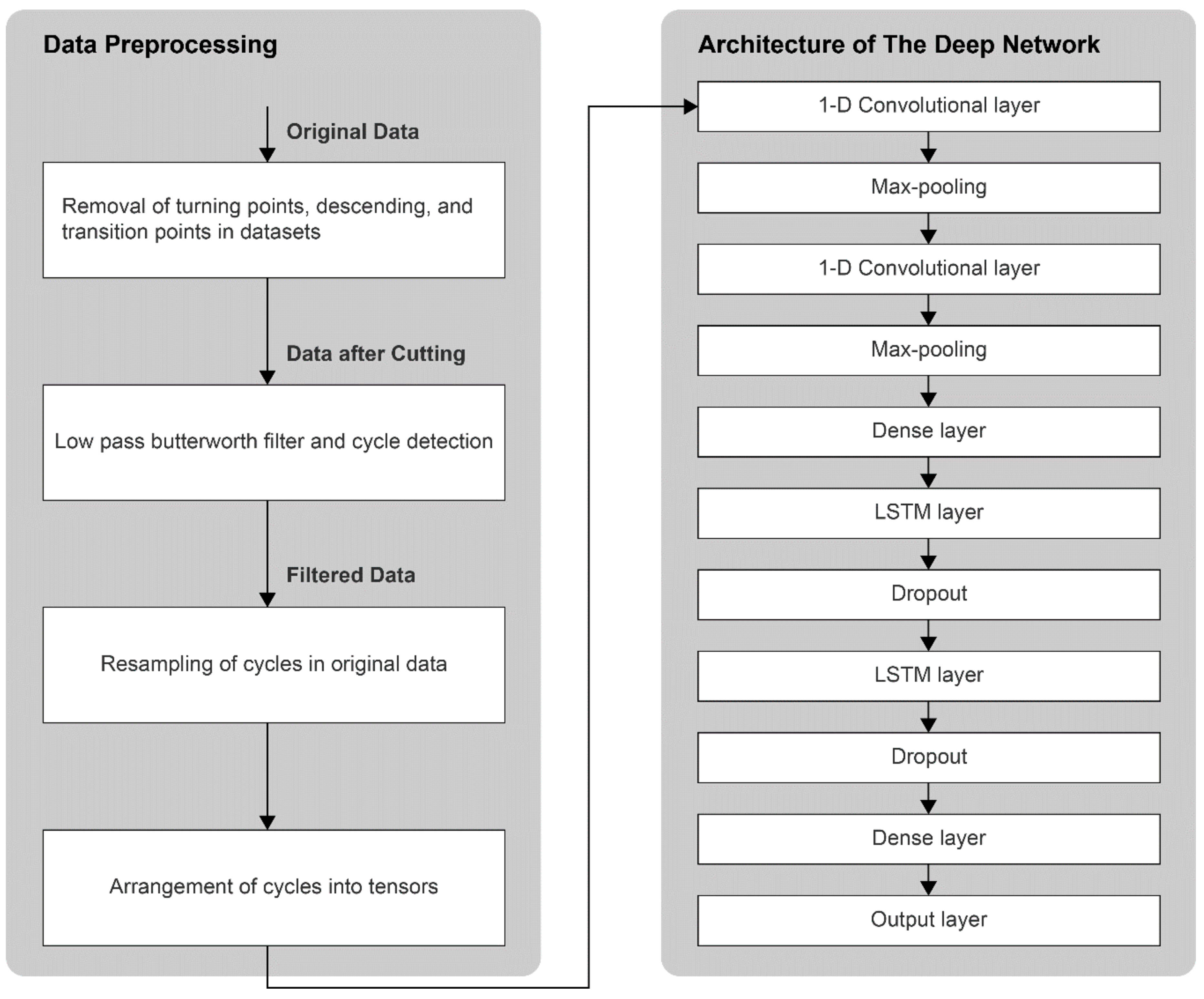
2.3. Data Selection and Preprocessing
2.3.1. Training Dataset
2.3.2. Validation Dataset
2.3.3. Test Dataset
2.4. Architecture of the Deep Network
3. Results
3.1. Training and Validation Set Results Using Deep Learning
3.2. Leave-One-Out Testing Results
3.3. Test Set Result Using Deep Learning
3.4. Validation and Test Set Results Using K-Nearest Neighbors Algorithm
4. Discussion
5. Conclusions
Author Contributions
Funding
Acknowledgments
Conflicts of Interest
Appendix A
Appendix A.1

| Predicted | DS | P-Off | KDP | DP | V2 | V2A | V1 | FS | |
|---|---|---|---|---|---|---|---|---|---|
| True | |||||||||
| DS | 190 | 0 | 0 | 0 | 0 | 0 | 0 | 0 | |
| P-Off | 0 | 0 | 0 | 0 | 0 | 0 | 0 | 0 | |
| KDP | 0 | 0 | 7 | 0 | 0 | 0 | 0 | 0 | |
| DP | 0 | 2 | 9 | 49 | 1 | 2 | 0 | 0 | |
| V2 | 0 | 0 | 0 | 0 | 0 | 0 | 0 | 0 | |
| V2A | 0 | 0 | 0 | 0 | 0 | 0 | 0 | 0 | |
| V1 | 0 | 0 | 0 | 0 | 0 | 0 | 0 | 0 | |
| FS | 0 | 0 | 0 | 0 | 0 | 0 | 0 | 0 | |
| Predicted | DS | P-Off | KDP | DP | V2 | V2A | V1 | FS | |
|---|---|---|---|---|---|---|---|---|---|
| True | |||||||||
| DS | 0 | 0 | 0 | 0 | 0 | 0 | 0 | 0 | |
| P-Off | 0 | 0 | 0 | 0 | 0 | 0 | 0 | 0 | |
| KDP | 0 | 0 | 0 | 0 | 0 | 0 | 0 | 0 | |
| DP | 0 | 0 | 0 | 0 | 0 | 0 | 0 | 0 | |
| V2 | 0 | 0 | 0 | 2 | 93 | 3 | 0 | 0 | |
| V2A | 0 | 1 | 0 | 8 | 0 | 25 | 0 | 0 | |
| V1 | 0 | 1 | 1 | 0 | 4 | 0 | 593 | 3 | |
| FS | 0 | 0 | 0 | 0 | 0 | 0 | 0 | 0 | |
| Predicted | DS | P-Off | KDP | DP | V2 | V2A | V1 | FS | |
|---|---|---|---|---|---|---|---|---|---|
| True | |||||||||
| DS | 48 | 1 | 0 | 0 | 0 | 0 | 0 | 0 | |
| P-Off | 3 | 50 | 1 | 0 | 0 | 0 | 0 | 0 | |
| KDP | 2 | 3 | 20 | 1 | 0 | 0 | 0 | 0 | |
| DP | 0 | 0 | 0 | 0 | 0 | 0 | 0 | 0 | |
| V2 | 0 | 0 | 0 | 0 | 0 | 0 | 0 | 0 | |
| V2A | 0 | 0 | 0 | 0 | 0 | 0 | 0 | 0 | |
| V1 | 0 | 0 | 0 | 0 | 0 | 0 | 0 | 0 | |
| FS | 0 | 0 | 0 | 0 | 0 | 0 | 0 | 0 | |
| Predicted | DS | P-Off | KDP | DP | V2 | V2A | V1 | FS | |
|---|---|---|---|---|---|---|---|---|---|
| True | |||||||||
| DS | 0 | 0 | 0 | 0 | 0 | 0 | 0 | 0 | |
| P-Off | 0 | 0 | 0 | 0 | 0 | 0 | 0 | 0 | |
| KDP | 0 | 0 | 0 | 0 | 0 | 0 | 0 | 0 | |
| DP | 0 | 0 | 0 | 0 | 0 | 0 | 0 | 0 | |
| V2 | 0 | 0 | 0 | 0 | 10 | 2 | 1 | 0 | |
| V2A | 0 | 0 | 0 | 1 | 2 | 20 | 0 | 1 | |
| V1 | 0 | 0 | 1 | 0 | 2 | 0 | 12 | 0 | |
| FS | 0 | 0 | 0 | 0 | 0 | 1 | 0 | 9 | |
Appendix A.2
| Predicted | DS | P-Off | KDP | DP | V2 | V2A | V1 | FS | |
|---|---|---|---|---|---|---|---|---|---|
| True | |||||||||
| DS | 0 | 0 | 0 | 0 | 0 | 0 | 0 | 0 | |
| P-Off | 0 | 0 | 0 | 0 | 0 | 0 | 0 | 0 | |
| KDP | 0 | 0 | 0 | 0 | 0 | 0 | 0 | 0 | |
| DP | 0 | 0 | 0 | 0 | 0 | 0 | 0 | 0 | |
| V2 | 0 | 0 | 0 | 2 | 34 | 15 | 8 | 1 | |
| V2A | 0 | 0 | 0 | 0 | 2 | 27 | 2 | 0 | |
| V1 | 0 | 0 | 0 | 0 | 5 | 30 | 158 | 4 | |
| FS | 0 | 0 | 0 | 0 | 0 | 0 | 0 | 0 | |
| Predicted | DS | P-Off | KDP | DP | V2 | V2A | V1 | FS | |
|---|---|---|---|---|---|---|---|---|---|
| True | |||||||||
| DS | 30 | 1 | 2 | 0 | 0 | 0 | 0 | 0 | |
| P-Off | 0 | 10 | 1 | 2 | 0 | 0 | 0 | 0 | |
| KDP | 1 | 3 | 35 | 0 | 0 | 0 | 0 | 0 | |
| DP | 0 | 0 | 0 | 0 | 0 | 0 | 0 | 0 | |
| V2 | 0 | 0 | 0 | 0 | 0 | 0 | 0 | 0 | |
| V2A | 0 | 0 | 0 | 0 | 0 | 0 | 0 | 0 | |
| V1 | 0 | 0 | 0 | 0 | 0 | 0 | 0 | 0 | |
| FS | 0 | 0 | 0 | 0 | 0 | 0 | 0 | 0 | |
| Predicted | DS | P-Off | KDP | DP | V2 | V2A | V1 | FS | |
|---|---|---|---|---|---|---|---|---|---|
| True | |||||||||
| DS | 0 | 0 | 0 | 0 | 0 | 0 | 0 | 0 | |
| P-Off | 0 | 0 | 0 | 0 | 0 | 0 | 0 | 0 | |
| KDP | 0 | 0 | 0 | 0 | 0 | 0 | 0 | 0 | |
| DP | 0 | 0 | 0 | 0 | 0 | 0 | 0 | 0 | |
| V2 | 0 | 0 | 0 | 0 | 19 | 21 | 4 | 0 | |
| V2A | 0 | 0 | 0 | 0 | 3 | 54 | 0 | 3 | |
| V1 | 0 | 0 | 0 | 0 | 0 | 0 | 7 | 0 | |
| FS | 0 | 0 | 0 | 1 | 0 | 2 | 3 | 15 | |
Appendix A.3
| Sensor Configuration | Course & Technique | Natural Course | Flat Course | Mean Accuracy | ||||
|---|---|---|---|---|---|---|---|---|
| Skier | Classical Style | Skating Style | Classical Style | Skating Style | ||||
| Whole body sensors (17) | Skier 1 | X | 89.4% | 82.3% | 76.5% | 82.7% | ||
| Skier 2 | 97.7% | 96.2% | 84.5% | 88.7% | 91.8% | |||
| Skier 3 | 92.4% | 61.4% | 82.9% | 54.8% | 72.9% | |||
| Mean Accuracy | 95.0% | 82.3% | 83.2% | 73.3% | ~83.0% | |||
| Upper body sensors (11) | Skier 1 | X | 82.4% | 67.6% | 74.2% | 74.7% | ||
| Skier 2 | 73.5% | 68.8% | 76.5% | 64.1% | 70.7% | |||
| Skier 3 | 66.2% | 42.3% | 78.5% | 44.1% | 57.8% | |||
| Mean Accuracy | 69.9% | 64.5% | 74.2% | 60.8% | ~68% | |||
| Lower body sensors (7) | Skier 1 | X | 24.2% | 74.9% | 66.3% | 55.1% | ||
| Skier 2 | 94.6% | 24.2% | 86.8% | 67.7% | 68.3% | |||
| Skier 3 | 91.1% | 68.7% | 86.2% | 50.5% | 74.1% | |||
| Mean Accuracy | 92.9% | 39.0% | 82.6% | 61.5% | ~66% | |||
| Pelvis sensor only (1) | Skier 1 | X | 24.0% | 77.6% | 56.1% | 52.6% | ||
| Skier 2 | 64.6% | 85.3% | 51.1% | 38.7% | 59.9% | |||
| Skier 3 | 62.4% | 20.2% | 82.1% | 21.5% | 46.5% | |||
| Mean Accuracy | 63.5% | 43.1% | 70.3% | 38.8% | ~53% | |||
| Sensor Configuration | Course & Technique | Natural Course | Flat Course | Mean Accuracy | |||
|---|---|---|---|---|---|---|---|
| Skier | Classical Style | Skating Style | Classical Style | Skating Style | |||
| Whole body sensors (17) | Skier 1 | X | 89.1% | 65.2% | 65.4% | 73.2% | |
| Skier 2 | 69.5% | 82.6% | 60.8% | 78.7% | 72.9% | ||
| Skier 3 | 81.4% | 74.4% | 70.2% | 56.3% | 70.6% | ||
| Mean Accuracy | 75.5% | 82.0% | 65.4% | 66.8% | ~72% | ||
| Upper body sensors (11) | Skier 1 | X | 50.3% | 46.4% | 61.1% | 52.6% | |
| Skier 2 | 66.8% | 51.7% | 61.3% | 58.7% | 59.6% | ||
| Skier 3 | 64.4% | 73.3% | 49.6% | 55.3% | 60.7% | ||
| Mean Accuracy | 65.6% | 58.4% | 52.4% | 58.4% | ~59% | ||
| Lower body sensors (7) | Skier 1 | X | 81.3% | 56.5% | 50.7% | 62.8% | |
| Skier 2 | 49.8% | 51.7% | 48.8% | 38.7% | 47.3% | ||
| Skier 3 | 81.1% | 38.9% | 62.6% | 36.9% | 54.9% | ||
| Mean Accuracy | 65.4% | 57.3% | 56.0% | 42.1% | ~55% | ||
| Pelvis sensor only (1) | Skier 1 | X | 2.4% | 30.4% | 2.1% | 11.7% | |
| Skier 2 | 21.8% | 10.9% | 15.7% | 9.3% | 14.5% | ||
| Skier 3 | 40.1% | 2.9% | 24.4% | 7.8% | 18.8% | ||
| Mean Accuracy | 30.9% | 5.4% | 23.5% | 6.4% | ~15% | ||
References
- Rindal, O.M.H.; Seeberg, T.M.; Tjønnås, J.; Haugnes, P.; Sandbakk, Ø. Automatic classification of sub-techniques in classical cross-country skiing using a machine learning algorithm on micro-sensor data. Sensors 2017, 18, 75. [Google Scholar] [CrossRef] [PubMed]
- Andersson, E.; Pellegrini, B.; Sandbakk, O.; Stuggl, T.; Holmberg, H.C. The effects of skiing velocity on mechanical aspects of diagonal cross-country skiing. Sports Biomech. 2014, 13, 267–284. [Google Scholar] [CrossRef] [PubMed]
- Bilodeau, B.; Boulay, M.R.; Roy, B. Propulsive and gliding phases in four cross-country skiing techniques. Med. Sci. Sports Exerc. 1992, 24, 917–925. [Google Scholar] [CrossRef] [PubMed]
- Bilodeau, B.; Rundell, K.W.; Roy, B.; Boulay, M.R. Kinematics of cross-country ski racing. Med. Sci. Sports Exerc. 1996, 28, 128–138. [Google Scholar] [CrossRef] [PubMed]
- Lindinger, S.J.; Gopfert, C.; Stoggl, T.; Muller, E.; Holmberg, H.C. Biomechanical pole and leg characteristics during uphill diagonal roller skiing. Sports Biomech. 2009, 8, 318–333. [Google Scholar] [CrossRef] [PubMed]
- Nilsson, J.; Tveit, P.; Eikrehagen, O. Effects of speed on temporal patterns in classical style and freestyle cross-country skiing. Sports Biomech. 2004, 3, 85–107. [Google Scholar] [CrossRef] [PubMed]
- Ohtonen, O.; Lindinger, S.; Lemmettylä, T.; Seppälä, S.; Linnamo, V. Validation of porTable 2d force binding systems for cross-country skiing. Sports Eng. 2013, 16, 281–296. [Google Scholar] [CrossRef]
- Stoggl, T.; Kampel, W.; Muller, E.; Lindinger, S. Double-push skating versus v2 and v1 skating on uphill terrain in cross-country skiing. Med. Sci. Sports Exerc. 2010, 42, 187–196. [Google Scholar] [CrossRef] [PubMed]
- Stoggl, T.; Muller, E.; Lindinger, S. Biomechanical comparison of the double-push technique and the conventional skate skiing technique in cross-country sprint skiing. J. Sports Sci. 2008, 26, 1225–1233. [Google Scholar] [CrossRef] [PubMed]
- Fasel, B.; Favre, J.; Chardonnens, J.; Gremion, G.; Aminian, K. An inertial sensor-based system for spatio-temporal analysis in classic cross-country skiing diagonal technique. J. Biomech. 2015, 48, 3199–3205. [Google Scholar] [CrossRef] [PubMed]
- Marsland, F.; Lyons, K.; Anson, J.; Waddington, G.; Macintosh, C.; Chapman, D. Identification of cross-country skiing movement patterns using micro-sensors. Sensors 2012, 12, 5047–5066. [Google Scholar] [CrossRef] [PubMed]
- Smith, G.A. Biomechanics of crosscountry skiing. Sports Med. 1990, 9, 273–285. [Google Scholar] [CrossRef] [PubMed]
- Marsland, F.; Mackintosh, C.; Holmberg, H.C.; Anson, J.; Waddington, G.; Lyons, K.; Chapman, D. Full course macro-kinematic analysis of a 10 km classical cross-country skiing competition. PLoS ONE 2017, 12, e0182262. [Google Scholar] [CrossRef] [PubMed]
- Marsland, F.; Mackintosh, C.; Anson, J.; Lyons, K.; Waddington, G.; Chapman, D.W. Using micro-sensor data to quantify macro kinematics of classical cross-country skiing during on-snow training. Sports Biomech. 2015, 14, 435–447. [Google Scholar] [CrossRef] [PubMed]
- Myklebust, H.; Nunes, N.; Hallén, J.; Gamboa, H. Morphological analysis of acceleration signals in cross-country skiing. In Proceedings of the Biosignals-International Conference on Bio-Inspired Systems and Signal Processing (BIOSTEC 2011), Rome, Italy, 26–29 January 2011; pp. 26–29. [Google Scholar]
- Sakurai, Y.; Fujita, Z.; Ishige, Y. Automated identification and evaluation of subtechniques in classical-style roller skiing. J. Sports Sci. Med. 2014, 13, 651–657. [Google Scholar] [PubMed]
- Sakurai, Y.; Fujita, Z.; Ishige, Y. Automatic identification of subtechniques in skating-style roller skiing using inertial sensors. Sensors (Basel) 2016, 16, 473. [Google Scholar] [CrossRef] [PubMed]
- Seeberg, T.M.; Tjonnas, J.; Rindal, O.M.H.; Haugnes, P.; Dalgard, S.; Sandbakk, O. A multi-sensor system for automatic analysis of classical cross-country skiing techniques. Sports Eng. 2017, 20, 313–327. [Google Scholar] [CrossRef]
- Stoggl, T.; Holst, A.; Jonasson, A.; Andersson, E.; Wunsch, T.; Norstrom, C.; Holmberg, H.C. Automatic classification of the sub-techniques (gears) used in cross-country ski skating employing a mobile phone. Sensors (Basel) 2014, 14, 20589–20601. [Google Scholar] [CrossRef] [PubMed]
- Ristner, M. A Comparison of a k-Nearest Neighbour and a Markov Model for Classification of Gears in Cross-Country Skiing. Available online: https://www.nada.kth.se/utbildning/grukth/exjobb/rapportlistor/2015/sammanf15/ristner_moa_eng.html (accessed on 4 October 2018).
- Holst, A.; Jonasson, A. Classification of Movement Patterns in Skiing; SCAI: Aalborg, Denmark, 2013; pp. 115–124. [Google Scholar]
- Yao, S.; Hu, S.; Zhao, Y.; Zhang, A.; Abdelzaher, T. Deepsense: A unified deep learning framework for time-series mobile sensing data processing. In Proceedings of the 26th International Conference on World Wide Web, Perth, Australia, 3–7 April 2017; International World Wide Web Conferences Steering Committee: Geneva, Switzerland; pp. 351–360. [Google Scholar]
- Rassem, A.; El-Beltagy, M.; Saleh, M. Cross-country skiing gears classification using deep learning. arXiv, 2017; arXiv:1706.08924. [Google Scholar]
- Andersson, E.; Supej, M.; Sandbakk, O.; Sperlich, B.; Stoggl, T.; Holmberg, H.C. Analysis of sprint cross-country skiing using a differential global navigation satellite system. Eur. J. Appl. Physiol. 2010, 110, 585–595. [Google Scholar] [CrossRef] [PubMed] [Green Version]


| Related Work | Number of Sensors/Locations | Subjects | Number of Classes (XC-Skiing Style) | Used Classification Method | Classification Accuracy | Data Acquisition Details |
|---|---|---|---|---|---|---|
| [18] | 6 inertial measurement units (IMUs)/upper back, lower back, left and right arm, left and right ankle; 1 sensor unit/chest (including 1 accelerometer, 1 gyroscope, 1 skin temperature sensor, 1 heart rate sensor) | 11 (10 males, 1 female) | 3 (classical style) | An algorithm based on the correlations of angle values of arms and legs | Sensitivity: 99~100% | Data collected in different types of tracks and snow conditions |
| [19] | 1 accelerometer/chest | 11 (7 males, 4 females) | 5 (skating style) | Machine Learning Model (Markov Chain of multivariate Gaussian distribution) | 86% ± 8.9% for collective data | Data collected on treadmill using roller skies (different speeds and inclines) |
| [20] | 1 accelerometer/chest | 3 skiers for the test set | Both classical style and skating style | Machine Learning Models (a Markov model and a KNN model) | The error rates for tests: 7.22% for the Markov model; 0.19% for KNN model | The test set for the cross-validation consists of 30 cycles from each gear from three different skiers in classical style and from three different skiers in skating style |
| [1] | 2 inertial sensors: 1 accelerometer/chest; 1 gyroscope/arm | 10 (9 males, 1 female) | 8 (classical style) | Neural Networks | 93.9% ± 3% for the test data | Data collected on treadmill and real competition course on snow |
| [21] | 1 accelerometer/chest | No details | 2 (skating style) | Neural Networks | CNN error rate: 2.4% LSTM error rate: 1.6% | No detailed information |
| Attribute | Gender | Age (in Years) | Weight (in kg) | Height (in cm) | |
|---|---|---|---|---|---|
| Skier | |||||
| 1 | Female | 24 | 51 | 163 | |
| 2 | Female | 22 | 51 | 162 | |
| 3 | Male | 23 | 69 | 176 | |
| Skier | Training Dataset | Validation Dataset | |||
|---|---|---|---|---|---|
| Flat Course; 1 Technique of Skating or Classical Style Repeatedly | Flat Course | Natural Course | |||
| Classical Style (DS, P-Off, KDP, DP) | Skating Style (V2, V2A, V1, FS) | Classical Style (DS, P-Off, KDP, DP) | Skating Style (V2, V2A, V1, FS) | ||
| Skier 1 | √ | √ | √ | X | √ |
| Skier 2 | √ | √ | √ | √ | √ |
| Skier 3 | √ | √ | √ | √ | √ |
| Technique | Classical Style | Skating Style | Sum | |||||||
|---|---|---|---|---|---|---|---|---|---|---|
| Skier | DS | P-Off | KDP | DP | V2 | V2A | V1 | FS | ||
| Skier 1 | 153 | 123 | 107 | 128 | 85 | 104 | 157 | 103 | 960 | |
| Skier 2 | 103 | 83 | 94 | 68 | 38 | 56 | 65 | 61 | 568 | |
| Skier 3 | 83 | 64 | 64 | 78 | 48 | 59 | 86 | 57 | 539 | |
| Sum | 339 | 270 | 265 | 274 | 171 | 219 | 308 | 221 | 2067 | |
| Skiing Course & Technique | Flat Course | Natural Course | ||
|---|---|---|---|---|
| Classical Style (DS, P-Off, KDP, DP) | Skating Style (V2, V2A, V1, FS) | Classical Style (DS, P-Off, KDP, DP) | Skating Style (V2, V2A, V1, FS) | |
| Skier 1 | 33, 13, 39, 0 | 44, 60, 7, 21 | X | 60, 31, 197, 0 |
| Skier 2 | 49, 0, 54, 26 | 13, 24, 15, 10 | 190, 0, 7, 63 | 98, 34, 602, 0 |
| Skier 3 | 16, 27, 34, 46 | 23, 32, 19, 19 | 145, 2, 5, 85 | 89, 30, 44, 0 |
| Test Set-1 Flat Course | Test Set-2 Natural Course | ||||||||||
|---|---|---|---|---|---|---|---|---|---|---|---|
| Classical Style | Skating Style | Skating Style | |||||||||
| DS | P-Off | KDP | DP | V2 | V2A | V1 | FS | V2 | V2A | V1 | FS |
| 649 | 511 | 378 | 569 | 366 | 447 | 631 | 480 | 72 | 13 | 219 | 0 |
| Sensor Configuration | Number of Sensors | Locations of Sensors |
|---|---|---|
| 1 | All 17 sensors (Whole-body) | Pelvis, chest, head, right and left shoulders, right and left upper arms, right and left forearms, right and left hands, right and left upper legs, right and left lower legs, right and left feet |
| 2 | 11 sensors (Upper body only) | Pelvis, chest, head, right and left shoulders, right and left upper arms, right and left forearms, right and left hands |
| 3 | 7 sensors (Lower body only) | Pelvis, right and left upper legs, right and left lower legs, right and left feet |
| 4 | 5 sensors (Sports biomechanics configuration) | Pelvis, right and left hands, right and left feet |
| 5 | 1 sensor (Pelvis only) | Pelvis |
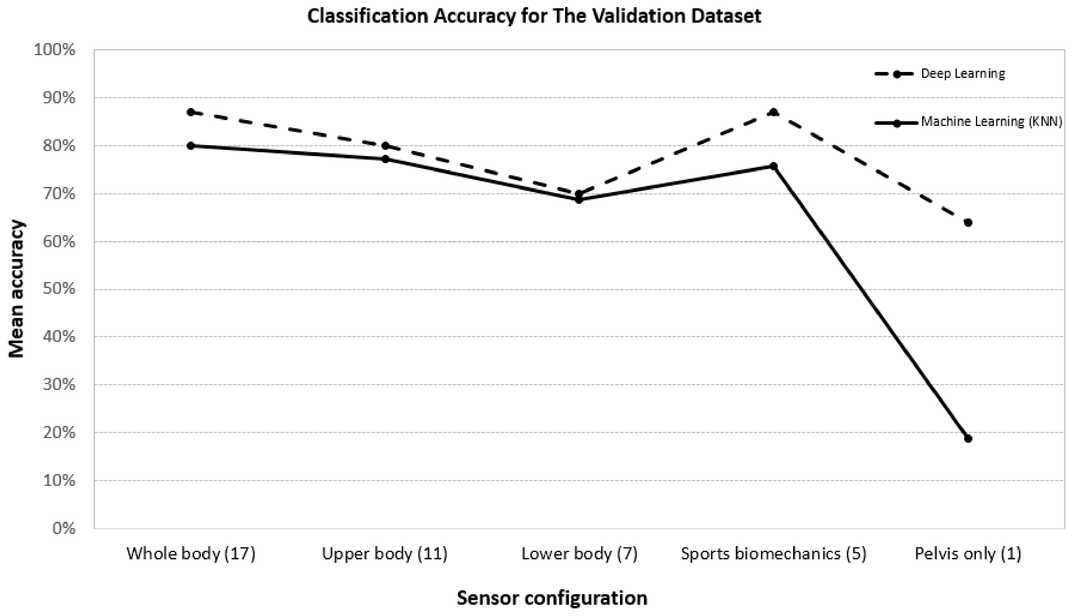
| Sensor Configuration | 17 Sensors (Whole Body) | 11 Sensors (Upper Body) | 7 Sensors (Lower Body) | 5 Sensors (Sports Biomech.) | 1 Sensor (Pelvis) |
|---|---|---|---|---|---|
| Accuracy | 99.39% | 97.96% | 98.03% | 97.82% | 79.4% |
| Predicted | DS | P-Off | KDP | DP | V2 | V2A | V1 | FS | |
|---|---|---|---|---|---|---|---|---|---|
| True | |||||||||
| DS | 339 | 0 | 0 | 0 | 0 | 0 | 0 | 0 | |
| P-Off | 0 | 242 | 0 | 28 | 0 | 0 | 0 | 0 | |
| KDP | 0 | 0 | 265 | 0 | 0 | 0 | 0 | 0 | |
| DP | 0 | 9 | 1 | 264 | 0 | 0 | 0 | 0 | |
| V2 | 0 | 1 | 0 | 1 | 168 | 0 | 1 | 0 | |
| V2A | 0 | 0 | 0 | 0 | 1 | 218 | 0 | 0 | |
| V1 | 0 | 0 | 0 | 0 | 3 | 0 | 305 | 0 | |
| FS | 0 | 0 | 0 | 0 | 0 | 0 | 0 | 221 | |
| Sensor Configuration | Course & Technique | Natural Course | Flat Course | Mean Accuracy | |||
|---|---|---|---|---|---|---|---|
| Skier | Classical Style | Skating Style | Classical Style | Skating Style | |||
| Whole body sensors (17) | Skier 1 | X | 89.58% | 78.82% | 76.52% | 81.64% | |
| Skier 2 | 97.31% | 97.68% | 89.15% | 79.03% | 90.79% | ||
| Skier 3 | 93.67% | 82.21% | 91.06% | 89.25% | 89.04% | ||
| Mean Accuracy | 95.49% | 89.82% | 86.34% | 81.60% | ~87.00% | ||
| Upper body sensors (11) | Skier 1 | X | 87.85% | 74.12% | 71.97% | 77.98% | |
| Skier 2 | 95.38% | 95.78% | 85.27% | 72.58% | 87.25% | ||
| Skier 3 | 66.24% | 82.21% | 73.17% | 88.17% | 77.45% | ||
| Mean Accuracy | 80.81% | 88.61% | 77.52% | 77.57% | ~80.00% | ||
| Lower body sensors (7) | Skier 1 | X | 54.86% | 78.82% | 52.27% | 61.98% | |
| Skier 2 | 92.31% | 25.34% | 85.27% | 69.35% | 68.07% | ||
| Skier 3 | 85.23% | 66.87% | 90.24% | 80.65% | 80.75% | ||
| Mean Accuracy | 88.77% | 49.02% | 84.78% | 67.42% | ~70.00% | ||
| Sports biomechanics configuration (5) | Skier 1 | X | 76.04% | 88.23% | 71.96% | 78.74% | |
| Skier 2 | 94.61% | 96.87% | 91.47% | 82.26% | 91.30% | ||
| Skier 3 | 96.62% | 82.21% | 88.62% | 92.47% | 89.98% | ||
| Mean Accuracy | 95.61% | 85.04% | 89.44% | 82.23% | ~87.00% | ||
| Pelvis sensor only (1) | Skier 1 | X | 74.20% | 80.21% | 59.30% | 71.24% | |
| Skier 2 | 56.37% | 78.79% | 74.44% | 52.36% | 64.81% | ||
| Skier 3 | 59.32% | 64.73% | 68.80% | 31.23% | 56.02% | ||
| Mean Accuracy | 57.85% | 72.57% | 74.48% | 47.63% | ~64.00% | ||
| Predicted | DS | P-Off | KDP | DP | V2 | V2A | V1 | FS | |
|---|---|---|---|---|---|---|---|---|---|
| True | |||||||||
| DS | 145 | 0 | 0 | 0 | 0 | 0 | 0 | 0 | |
| P-Off | 0 | 1 | 0 | 1 | 0 | 0 | 0 | 0 | |
| KDP | 0 | 0 | 4 | 0 | 1 | 0 | 0 | 0 | |
| DP | 1 | 1 | 0 | 79 | 1 | 3 | 0 | 0 | |
| V2 | 0 | 0 | 0 | 0 | 0 | 0 | 0 | 0 | |
| V2A | 0 | 0 | 0 | 0 | 0 | 0 | 0 | 0 | |
| V1 | 0 | 0 | 0 | 0 | 0 | 0 | 0 | 0 | |
| FS | 0 | 0 | 0 | 0 | 0 | 0 | 0 | 0 | |
| Predicted | DS | P-Off | KDP | DP | V2 | V2A | V1 | FS | |
|---|---|---|---|---|---|---|---|---|---|
| True | |||||||||
| DS | 0 | 0 | 0 | 0 | 0 | 0 | 0 | 0 | |
| P-Off | 0 | 0 | 0 | 0 | 0 | 0 | 0 | 0 | |
| KDP | 0 | 0 | 0 | 0 | 0 | 0 | 0 | 0 | |
| DP | 0 | 0 | 0 | 0 | 0 | 0 | 0 | 0 | |
| V2 | 0 | 0 | 0 | 0 | 86 | 3 | 0 | 0 | |
| V2A | 0 | 0 | 0 | 0 | 1 | 5 | 23 | 1 | |
| V1 | 0 | 0 | 0 | 0 | 1 | 0 | 43 | 0 | |
| FS | 0 | 0 | 0 | 0 | 0 | 0 | 0 | 0 | |
| Predicted | DS | P-Off | KDP | DP | V2 | V2A | V1 | FS | |
|---|---|---|---|---|---|---|---|---|---|
| True | |||||||||
| DS | 16 | 0 | 0 | 0 | 0 | 0 | 0 | 0 | |
| P-Off | 0 | 22 | 0 | 5 | 0 | 0 | 0 | 0 | |
| KDP | 0 | 6 | 27 | 1 | 0 | 0 | 0 | 0 | |
| DP | 0 | 0 | 1 | 44 | 1 | 0 | 0 | 0 | |
| V2 | 0 | 0 | 0 | 0 | 0 | 0 | 0 | 0 | |
| V2A | 0 | 0 | 0 | 0 | 0 | 0 | 0 | 0 | |
| V1 | 0 | 0 | 0 | 0 | 0 | 0 | 0 | 0 | |
| FS | 0 | 0 | 0 | 0 | 0 | 0 | 0 | 0 | |
| Predicted | DS | P-Off | KDP | DP | V2 | V2A | V1 | FS | |
|---|---|---|---|---|---|---|---|---|---|
| True | |||||||||
| DS | 0 | 0 | 0 | 0 | 0 | 0 | 0 | 0 | |
| P-Off | 0 | 0 | 0 | 0 | 0 | 0 | 0 | 0 | |
| KDP | 0 | 0 | 0 | 0 | 0 | 0 | 0 | 0 | |
| DP | 0 | 0 | 0 | 0 | 0 | 0 | 0 | 0 | |
| V2 | 0 | 0 | 1 | 0 | 20 | 1 | 1 | 0 | |
| V2A | 0 | 0 | 0 | 1 | 0 | 30 | 0 | 1 | |
| V1 | 0 | 0 | 0 | 0 | 1 | 0 | 17 | 1 | |
| FS | 0 | 0 | 0 | 0 | 0 | 0 | 0 | 19 | |
| Course & Technique | Natural Course | Flat Course | Mean Accuracy | |||
|---|---|---|---|---|---|---|
| Skier | Classical Style | Skating Style | Classical Style | Skating Style | ||
| Skier 1 | X | 90.35% | 76.48% | 74.50% | 80.44% | |
| Skier 2 | 76.20% | 97.70% | 68.65% | 85.68% | 82.06% | |
| Skier 3 | 90.28% | 78.50% | 79.70% | 55.00% | 75.87% | |
| Mean Accuracy | 83.24% | 88.85% | 74.94% | 71.73% | 79.69% | |
| Course & Technique | Natural Course | Flat Course | Mean Accuracy | |||
|---|---|---|---|---|---|---|
| Skier | Classical Style | Skating Style | Classical Style | Skating Style | ||
| Skier 1 | X | 86.05% | 57.25% | 58.33% | 67.21% | |
| Skier 2 | 75.09% | 87.76% | 50.38% | 53.33% | 66.64% | |
| Skier 3 | 83.71% | 56.98% | 57.25% | 37.86% | 58.95% | |
| Mean Accuracy | 79.40% | 76.93% | 54.96% | 49.84% | 65.28% | |
| Sensor Configuration | 17 Sensors (Whole Body) | 11 Sensors (Upper Body) | 7 Sensors (Lower Body) | 5 Sensors (Sports Biomech.) | 1 Sensor (Pelvis) |
|---|---|---|---|---|---|
| Test Set-1 | 84.21% | 84.80% | 84.35% | 87.20% | 58.54% |
| Test Set-2 | 92.18% | 84.83% | 64.58% | 95.10% | 29.65% |
| Mean Accuracy | 88.19% | 84.82% | 74.47% | 91.15% | 44.10% |
| Predicted | DS | P-Off | KDP | DP | V2 | V2A | V1 | FS | |
|---|---|---|---|---|---|---|---|---|---|
| True | |||||||||
| DS | 310 | 0 | 0 | 0 | 0 | 0 | 0 | 0 | |
| P-Off | 0 | 63 | 1 | 172 | 5 | 0 | 0 | 0 | |
| KDP | 0 | 0 | 113 | 0 | 0 | 0 | 0 | 0 | |
| DP | 0 | 74 | 0 | 221 | 0 | 0 | 0 | 0 | |
| V2 | 0 | 1 | 0 | 0 | 193 | 0 | 1 | 0 | |
| V2A | 0 | 0 | 0 | 1 | 4 | 221 | 2 | 0 | |
| V1 | 0 | 0 | 0 | 0 | 1 | 3 | 319 | 0 | |
| FS | 0 | 0 | 0 | 0 | 0 | 0 | 0 | 259 | |
| Predicted | DS | P-Off | KDP | DP | V2 | V2A | V1 | FS | |
|---|---|---|---|---|---|---|---|---|---|
| True | |||||||||
| DS | 0 | 0 | 0 | 0 | 0 | 0 | 0 | 0 | |
| P-Off | 0 | 0 | 0 | 0 | 0 | 0 | 0 | 0 | |
| KDP | 0 | 0 | 0 | 0 | 0 | 0 | 0 | 0 | |
| DP | 0 | 0 | 0 | 0 | 0 | 0 | 0 | 0 | |
| V2 | 0 | 0 | 0 | 1 | 66 | 2 | 3 | 0 | |
| V2A | 0 | 0 | 0 | 0 | 0 | 13 | 0 | 0 | |
| V1 | 0 | 0 | 0 | 0 | 6 | 1 | 210 | 2 | |
| FS | 0 | 0 | 0 | 0 | 0 | 0 | 0 | 2 | |
| Sensor Configuration | Course & Technique | Natural Course | Flat Course | Mean Accuracy | |||
|---|---|---|---|---|---|---|---|
| Skier | Classical Style | Skating Style | Classical Style | Skating Style | |||
| Whole body sensors (17) | Skier 1 | X | 60.54% | 61.59% | 60.54% | 60.89% | |
| Skier 2 | 91.70% | 97.50% | 83.67% | 80.00% | 88.22% | ||
| Skier 3 | 88.26% | 83.72% | 80.15% | 83.50% | 83.91% | ||
| Mean Accuracy | 89.98% | 80.59% | 75.14% | 74.68% | 80.10% | ||
| Upper body sensors (11) | Skier 1 | X | 66.33% | 47.83% | 66.32% | 60.16% | |
| Skier 2 | 84.43% | 93.95% | 77.56% | 88.00% | 85.99% | ||
| Skier 3 | 83.34% | 81.40% | 71.76% | 81.55% | 79.51% | ||
| Mean Accuracy | 83.89% | 80.56% | 65.72% | 78.62% | 77.20% | ||
| Lower body sensors (7) | Skier 1 | X | 68.37% | 58.70% | 68.37% | 65.15% | |
| Skier 2 | 82.70% | 38.55% | 77.56% | 64.00% | 65.70% | ||
| Skier 3 | 85.98% | 53.49% | 81.68% | 61.17% | 70.58% | ||
| Mean Accuracy | 84.34% | 53.47% | 72.65% | 64.51% | 68.74% | ||
| Sports biomechanics configuration (5) | Skier 1 | X | 50.68% | 52.17% | 50.68% | 51.18% | |
| Skier 2 | 86.85% | 95.92% | 83.67% | 81.34% | 86.95% | ||
| Skier 3 | 82.58% | 76.74% | 81.00% | 83.50% | 80.96% | ||
| Mean Accuracy | 84.72% | 74.45% | 72.28% | 71.84% | 75.82% | ||
| Pelvis sensor only (1) | Skier 1 | X | 2.72% | 25.36% | 2.08% | 10.05% | |
| Skier 2 | 31.83% | 31.18% | 15.74% | 10.67% | 22.36% | ||
| Skier 3 | 34.09% | 7.56% | 18.32% | 13.59% | 18.39% | ||
| Mean Accuracy | 32.96% | 13.82% | 19.81% | 8.78% | 18.84% | ||
| Sensor Configuration | 17 Sensors (Whole Body) | 11 Sensors (Upper Body) | 7 Sensors (Lower Body) | 5 Sensors (Sports Biomech.) | 1 Sensor (Pelvis) |
|---|---|---|---|---|---|
| Test Set-1 | 48.06% | 33.58% | 65.54% | 68.82% | 38.13% |
| Test Set-2 | 86.82% | 71.96% | 71.28% | 78.04% | 7.43% |
| Sensor Configuration | 17 Sensors (Whole Body) | 11 Sensors (Upper Body) | 7 Sensors (Lower Body) | 5 Sensors (Sports Biomech.) | 1 Sensor (Pelvis Body) | |||||
|---|---|---|---|---|---|---|---|---|---|---|
| Modeling method | ML-KNN | DL | ML-KNN | DL | ML-KNN | DL | ML-KNN | DL | ML-KNN | DL |
| Test set-1 | 48.1% | 84.2% | 33.6% | 84.8% | 65.5% | 84.4% | 68.8% | 87.2% | 38.1% | 58.5% |
| Test set-2 | 86.8% | 92.2% | 72.0% | 84.8% | 71.3% | 64.6% | 78.0% | 95.1% | 7.4% | 29.7% |
© 2018 by the authors. Licensee MDPI, Basel, Switzerland. This article is an open access article distributed under the terms and conditions of the Creative Commons Attribution (CC BY) license (http://creativecommons.org/licenses/by/4.0/).
Share and Cite
Jang, J.; Ankit, A.; Kim, J.; Jang, Y.J.; Kim, H.Y.; Kim, J.H.; Xiong, S. A Unified Deep-Learning Model for Classifying the Cross-Country Skiing Techniques Using Wearable Gyroscope Sensors. Sensors 2018, 18, 3819. https://doi.org/10.3390/s18113819
Jang J, Ankit A, Kim J, Jang YJ, Kim HY, Kim JH, Xiong S. A Unified Deep-Learning Model for Classifying the Cross-Country Skiing Techniques Using Wearable Gyroscope Sensors. Sensors. 2018; 18(11):3819. https://doi.org/10.3390/s18113819
Chicago/Turabian StyleJang, Jihyeok, Ankit Ankit, Jinhyeok Kim, Young Jae Jang, Hye Young Kim, Jin Hae Kim, and Shuping Xiong. 2018. "A Unified Deep-Learning Model for Classifying the Cross-Country Skiing Techniques Using Wearable Gyroscope Sensors" Sensors 18, no. 11: 3819. https://doi.org/10.3390/s18113819