N-Dimensional LLL Reduction Algorithm with Pivoted Reflection


School of Electronic Engineering, Beijing University of Posts and Telecommunications, No. 10 Xitucheng Road, Beijing 100876, China
*
Author to whom correspondence should be addressed.
Sensors 2018, 18(1), 283; https://doi.org/10.3390/s18010283
Submission received: 18 December 2017
/
Revised: 12 January 2018
/
Accepted: 14 January 2018
/
Published: 19 January 2018
(This article belongs to the Section Remote Sensors)
Abstract
:The Lenstra-Lenstra-Lovász (LLL) lattice reduction algorithm and many of its variants have been widely used by cryptography, multiple-input-multiple-output (MIMO) communication systems and carrier phase positioning in global navigation satellite system (GNSS) to solve the integer least squares (ILS) problem. In this paper, we propose an n-dimensional LLL reduction algorithm (n-LLL), expanding the Lovász condition in LLL algorithm to n-dimensional space in order to obtain a further reduced basis. We also introduce pivoted Householder reflection into the algorithm to optimize the reduction time. For an m-order positive definite matrix, analysis shows that the n-LLL reduction algorithm will converge within finite steps and always produce better results than the original LLL reduction algorithm with n > 2. The simulations clearly prove that n-LLL is better than the original LLL in reducing the condition number of an ill-conditioned input matrix with 39% improvement on average for typical cases, which can significantly reduce the searching space for solving ILS problem. The simulation results also show that the pivoted reflection has significantly declined the number of swaps in the algorithm by 57%, making n-LLL a more practical reduction algorithm.
1. Introduction
With the rapid development of the Beidou System (BDS), the Galileo system, the Global Positioning System (GPS) and the GLONASS system, the Global Navigation Satellite System (GNSS) is serving more and more people with higher positioning accuracy [1,2]. Alongside the standard point positioning, carrier-phase based precise positioning techniques with cm-level to mm-level accuracy, such like real-time kinematic (RTK) and precise point positioning (PPP), have started to show their potential in public services other than in specific areas such as ground surveying. The commercial continuous operational reference station (CORS) network providers have enabled the precise positioning applications in unmanned aerial vehicle (UAV), unmanned autonomous vehicle and so on [3,4,5].
The main computational effort in carrier-phase precise positioning is to resolve the carrier phase integer ambiguity which is contaminated by all kind of noises during the signal propagation. Several efficient ambiguity resolution methods were proposed during the last several decades such as: Least-Square Ambiguity Searching Technique (LSAST) [6], Triple Frequency Ambiguity Resolution (TCAR) [7], Least-squares AMBiguity Decorrelation Adjustment (LAMBDA) [8,9]. The great breakthrough of LAMBDA algorithm is bringing the “decorrelation” process into integer ambiguity resolution, dividing the whole process into: estimation, decorrelation (also known as Z-transformation), search and back transformation.
As the measurements of pseudo-range and carrier phase are strongly correlated in time and space, the coefficient matrix to resolve the ambiguities is so ill-conditioned that the search space is huge and abnormal, making the search process extremely time-consuming and inefficient. For real-time applications, the decorrelation process is curial to reduce search effort. As for LAMBDA, integer Gauss transformation with permutation is used as the decorrelation process and is proven to be very effective. A series of algorithms have been applied to the decorrelation process since then. Xu used Cholesky decomposition to calculate the Z-transformation matrix [10]; Chang modified the Gauss transformation in LAMBDA with symmetric pivoting strategy [11]; Xu proposed the parallel Cholesky-based reduction method using minimum pivoting strategy [12] and Hassibi was the first to introduce LLL algorithm into integer ambiguity resolution [13].
The LLL reduction algorithm was first proposed by Arjen Lenstra, Hendrik Lenstra and László Lovász in 1982 [14] and had been proven useful polynomial-time algorithm to solve the closest vector problem (CVP) since then. With the development of lattice theory and its application, LLL algorithm becomes a powerful tool to solve the ILS problem, which expands its usage to numerous applications such like next generation MIMO communication detection algorithm [15,16,17], integer ambiguity resolution [13,18] and many other integer solution finding problem.
The original LLL reduction algorithm uses Gram-Schmidt orthogonalization to generate orthogonal basis, which involves O(nlog(B))-bit integer. A float point LLL (FPLLL) algorithm is proposed to avoid the waste of resources [19]. Schnorr used the half-k method [20] to ensure the calculation accuracy with FPLLL, which only involves O(n + log(B))-bit integer and converges in O(n4log(B)). Koy proposed a segment LLL algorithm, weakening the constraints of reduction to ensure the efficiency of the algorithm when dealing with matrix of rank 350 or above. Schnoor proposed the deep insertion LLL (DeepLLL) and the Block Korkine-Zolotareff (BKZ) algorithm [21], which improved the performance significantly. Fontein made the DeepLLL algorithm a polynomial-time algorithm with the help of potential factor, naming it potential LLL (PotLLL) [22].
In this paper, we propose the n-LLL reduction, expanding the Lovász condition of original LLL algorithm to n-dimensional space. And we give out an adjustable parameter “n” to balance the performance and computational efforts. Pivoted Householder reflection and Givens transformation are also introduced into the n-LLL algorithm to further optimize the reduction time.
The performance and complexity of the n-LLL algorithm are then analyzed, showing that the new algorithm performs better than the original LLL algorithm with n > 2 and will always converge in polynomial time. The simulation results show that the n-LLL algorithm has better reduction quality than the original LLL with about 39% improvement on average. The new algorithm causes no significant increase in computational efforts because of the pivoted reflection, which is able to reduce as much as 57% swaps in the algorithm.
2. The LLL Reduction
A lattice is defined as:
where denote m independent liner vectors defined on and are called a basis of lattice . So, a lattice can be seen as a discrete point set inside the real value space .
Then the typical weighted ILS problem like:
can be described as: finding a vector that is closest to ( is the covariance matrix of vector ), which is also known as a CVP. As a CVP is an NP-hard problem, one efficient approach to acquire an approximate solution is lattice basis reduction. To simplify the demonstration, the discussions below involve only square matrix.
For a basis of lattice , obviously is also a basis of , where is a unimodular matrix. Then the weighted ILS problem (2) can be rewritten as:
where:
Assuming that we are able to find a proper unimodular matrix that makes all the column vectors of mutually orthogonal, the optimized solution of can be obtained by rounding each entry in and the solution for can be calculated accordingly, which is also known as the Babai’s method [23]. However, such kind of matrix cannot be found in general cases. As a result, the best way we can do is to find an approximate solution for matrix that makes as orthogonal as possible and the column vectors as short as possible, which is the so called “reduction” process.
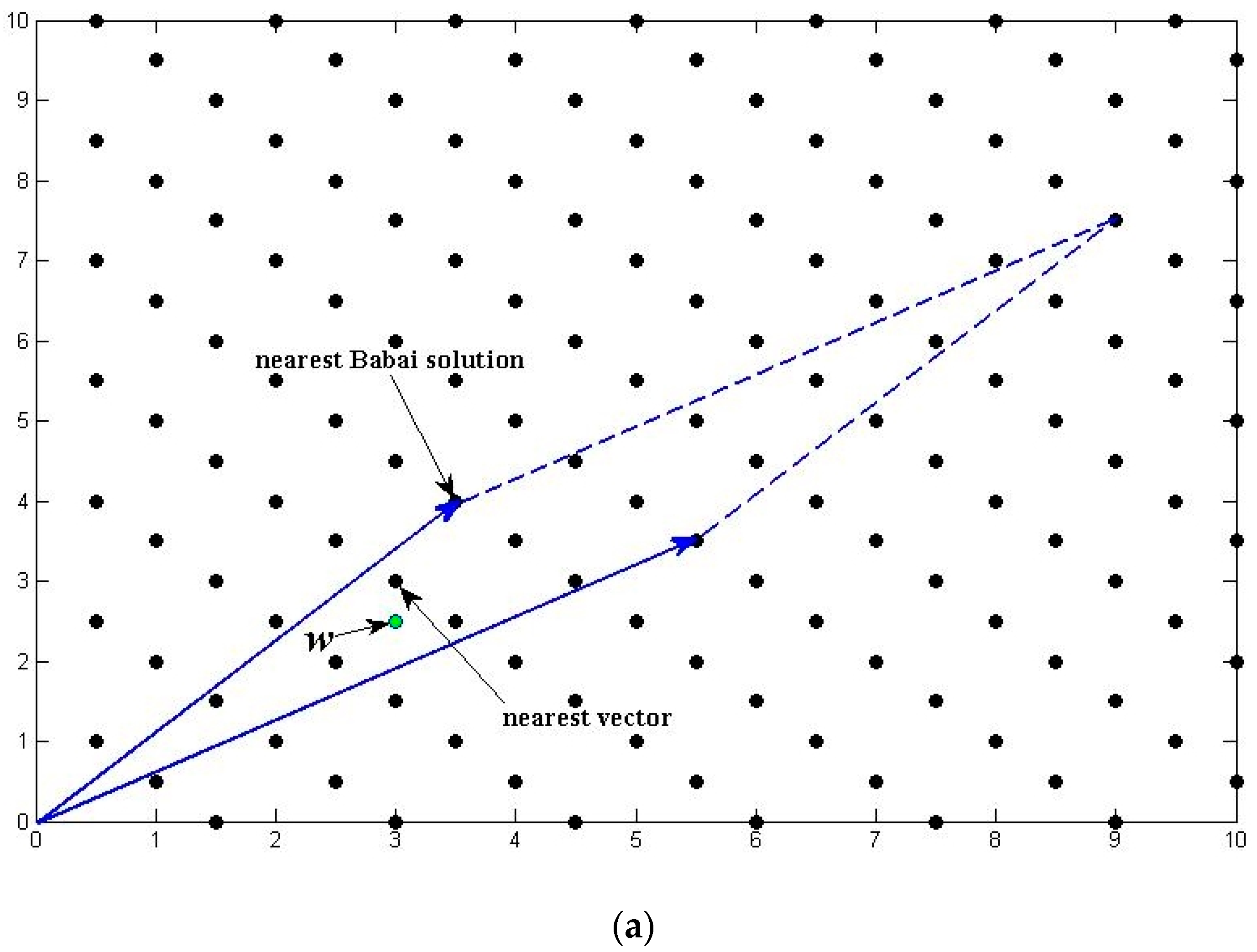
Figure 1 shows the difference between a “bad” and a “good” reduced lattice basis and how they affect the search process. The basis vectors in Figure 1a are relatively long and have smaller angle, which will bring larger error when estimating the CVP solution for real value vector . On the contrary, the basis vectors in Figure 1b are mutually orthogonal, enabling the Babai’s method to find the solution instantly.
2.1. The LLL Reduction Algorithm
The two primary goals of reduction process are:
- To make the column vectors in as mutually orthogonal as possible. As mentioned above, if the vectors are mutually orthogonal, then a simple rounding process will solve the ILS problem. Thus, the orthogonality of the vectors actually defines shape of search space, which will have significant influence on search efficiency;
- To minimize the length of vectors . Note that gives an upper bound of the volume of searching space, which means minimizing the vector length will shrinking the search space.
With the two goals, several reduction algorithm were proposed in the last decades and among those was the most famous LLL reduction algorithm proposed by Lenstra et al. [14].
The LLL reduction algorithm is consisted of two parts: size reduction and vector swap. The size reduction uses Gram-Schmidt orthogonalization. Let be a basis of lattice and a Gram-Schmidt basis can be described as:
where:
Definition 1.
Given a basis of lattice and its Gram-Schmidt orthogonal matrix
,
is LLL reduced if it satisfies the following two conditions:
where parameter
satisfies
.
The LLL reduction algorithm starts with setting and then is replaced by if for to satisfy the size condition (7). If Lovász condition (8) is violated for , then the column vectors and are swapped and the size reduction process will go back to again. After as much as iterations [14], when the Lovász condition is satisfied between and , the LLL reduction is done.
As we can see from the process of LLL reduction algorithm shown in Algorithm 1, the size reduction process adjusts the angle of by rounded Gram-Schmidt orthogonalization and the length of is reduced at the same time.
| Algorithm 1: The LLL reduction algorithm |
| Set |
| Set i = 2 |
| For |
| For j = 1 to i − 1 |
| Set = (Size reduction) |
| End |
| If then (Lovász condition) |
| Swap (, ) (Swap process) |
| Set i = max(i − 1, 2) |
| Else |
| Set i = i + 1 |
| End |
| End |
Clearly, the performance of size reduction process is strongly dependent on the order of the column vectors. Putting shorter vectors ahead will help improving the performance because shorter vectors kind of “push” the vectors after them to a more orthogonal angle in order to satisfy the size condition. Ideally, if we have:
and then the lattice can be most reduced. But unfortunately, there is still no algorithm can achieve (9) in polynomial time. As a result, Lovász set the condition to (8), where is usually set to 0.75 [14], in order to make the algorithm finish within polynomial time.
2.2. The LLL Reduction with Pivoted Reflection
As can be seen from Algorithm 1, the loop indicator i decreases only when the swaps take place, which means the number of iterations is highly dependent on the number of swaps. Hence, if the column vectors are in ascending order or at least as ascending ordered as possible before the LLL reduction is executed, the number of swaps as well as the reduction time will surely decline.
Motivated by Chang’s MLAMBDA [11] which utilizes the symmetric pivoting strategy to improve the efficiency of the reduction process and Wübben’s MMSE Sorted QR decomposition [24] which extends the V-BLAST algorithm, we introduce the pivoted reflection strategy into LLL algorithm to pre-sort the column vectors.
As the Gram-Schmidt orthogonalization process in the original LLL algorithm is not an isometric process, the pivoting of the vectors has limited influence on the reduction time. Therefore, we chose the Householder transformation which is an elementary reflection transformation proposed by Turnbull and Aitken in 1932. The typical usage of the Householder reflection is QR decomposition. Given a none-zero vector , one can construct vector with and . Then the transformation matrix can be constructed as:
Assuming i − 1 vectors of have been transformed and is the submatrix:
then the ith transformation matrix can be calculated as:
where is the transformation matrix for submatrix according to (10). Then we get:
with , where is an orthogonal matrix and is an upper triangle matrix.
In order to make the column vectors as ascending ordered as possible, before each Householder transformation the shortest vector in submatrix is moved ahead and the corresponding column vector in is swapped with accordingly. The whole LLL reduction with pivoted reflection is given in Algorithm 2.
| Algorithm 2: The LLL reduction with pivoted reflection |
| Set and |
| For i = 1 to m − 1 (Pivoted Householder Reflection) |
| Find the shortest vector in |
| Swap(, ) of |
| Calculate for |
| Set and |
| End |
| Set k = 2 |
| While |
| For j = k-1 down to 1 |
| Set = (Size reduction) |
| End |
| If then (Lovász condition) |
| Swap (,) (Swap process) |
| Calculate for |
| Set and |
| Set k = max(k − 1, 2) |
| Else |
| Set k = k + 1 |
| End |
| End |
Furthermore, the algorithm can be more efficient by applying Givens transformation to the rotations in the swap process instead of Householder reflection, because only needs to be transformed to zero when swapping and . It should also be emphasized that the pivoted reflection strategy does not always sort the vectors in perfect ascending order, because the reflection on also transforms the vectors after it, which may create shorter vector. But as can be seen in the simulations in Section 4, the pivoted reflection is proved to be very effective in minimizing the number of vector swaps in LLL algorithm in many cases of interest.
3. N-Dimensional Expansion of LLL Reduction
As discussed at the end of Section 2.1, the reduction quality and the improvement of search space are both highly dependent on the order of the basis vectors. We propose the n-LLL reduction algorithm, which inherits the basic outline of the LLL reduction algorithm and strengths the constraint of the order of basis vectors.
3.1. The N-Dimensional LLL Reduction Algorithm
Look back at the two conditions of LLL reduction again:
and the reduction process can be described in another way as: applying a series of Gaussian reductions in the 2-dimensional lattice spanned by a Lovász condition optimized vector pair and .
However, the Lovász condition here only focuses on local optimization within two neighbor vectors which ignores the global optimization. In order to improve the effect of the optimization to enhance the ordering constraint, we extend the 2-dimensional condition to n-dimension. Like the LLL reduction defined in Definition 1, the n-dimensional LLL reduction is defined as:
Definition 2.
Given a basis of Lattice
and its Gram-Schmidt orthogonal matrix , is n-LLL reduced () if it satisfy the following two conditions:
where parameter satisfies: .
Condition (15) can also be rewritten as:
where is the column vector in submatrix and implies the length of the shortest none-zero vector in .
Both condition (15) and (16) ensure that is the optimized choice in the following n vectors, which brings stronger constraint to the reduced basis than the original Lovász condition. The n-LLL reduction becomes LLL reduction when n = 2.
Note that the extend Lovász condition in the n-LLL reduction is similar to Block Korkine-Zolotarev (BKZ) [21] reduction that applies Korkine-Zolotarev (KZ) reduction within a k-block. This paper extends the original Lovász condition instead of introducing KZ reduction basis.
As the constraint in n-LLL is stronger than in the original one, the increase of reduction time is predictable. Thus, pivoted reflection mentioned in Section 2.2 plays a vital role in controlling the total reduction time of the algorithm. So, we fuse QR decomposition and reduction together by deeply coupling the pivoted reflection and n-LLL reduction process.
One possible algorithm to achieve n-LLL reduction is shown in Algorithm 3:
| Algorithm 3: The n-LLL reduction with pivoted reflection |
| Set and |
| (Move the shortest vector to ) |
| Find the shortest vector in |
| Swap(,) of |
| Calculate for |
| Set and |
| Set i = 2 |
| While (Pivoted reflection and reduction process) |
| Find the shortest vector in |
| Swap(, ) of |
| Set temp = i |
| For j = i − 1 down to 1 |
| Set = (Size reduction) |
| If and i − j < n then (Extended Lovász condition) |
| Swap (, ) (Swap process) |
| Set temp = j |
| End |
| End |
| Calculate for |
| Set and |
| If i ! = temp then |
| i = temp |
| Else |
| Set i = i + 1 |
| End |
| End |
The algorithm above uses the “Pivoting-Reduction-Reflection” strategy for each vector of instead of “Pivoting-Reflection and Reduction” strategy of Algorithm 2. The pivoting process in the fusion strategy gives better result as it takes the influence of the rotations in vector swap into consideration. Note that vector may have less than zero entries because the vector pivoted to has not been reflected yet. However, as the Householder reflection is an isometry, it will not be a problem in the swap process. The vector is then reflected after swapped to a proper place. The whole algorithm is actually executing the pivoted QR decomposition and n-LLL reduction in parallel, making it more efficient.
3.2. Analysis
3.2.1. The Performance
The n-LLL reduction algorithm strengthens the Lovász condition, which will certainly improve the quality of reduced basis. In this section, the performance improvement between the n-LLL and LLL reduction is detailed analyzed.
In order to compare the performance of reduction algorithm, we need to introduce measures to evaluate the reduction quality. As the size reduction processes of the two algorithms are the same, we only need to compare the orthogonality of the reduced basis according to the two goals mentioned in Section 2. One of the mostly used way to measure the orthogonality defects is imported from the Hadamard inequality:
Theorem 1.
(Hadamard Inequality): Given a lattice and one of its basis , we have:
and it becomes an equation if and only if all the vectors are mutually orthogonal. Then, the orthogonality defect factor can be defined as:
with [25].
According to (15), we have:
and the size reduction process makes sure that . As a result, (19) can be rewritten as:
which means:
······
By combining (23) and (20), we can get:
Repeatedly:
Furthermore, by substituting (25) into the Gram-Schmidt orthogonalization (5), we get:
where denotes the integer no larger than . By considering , (26) can be further rewritten to:
Then the orthogonality defect factor is calculated:
It can be seen clearly from (28) and (25) that the upper bound of the orthogonality defect factor declines as the parameter n increasing, which proves that the reduction quality of n-LLL reduction algorithm with n > 2 is better than the original LLL reduction (which is equivalent to 2-LLL).
It should be emphasized that the orthogonality does not directly affect the search time according to [26,27]. However, as the two algorithms compared through the orthogonality defect factor share the same size reduction constraint, the difference of the factor actually measures the performance of vector ordering, or in another way measures the efficiency of size reduction. So, the conclusion of (28) still holds in numerical simulations in Section 4.
3.2.2. The Complexity
As can be seen in Algorithm 3, the loop indicator i goes back to temp after each vector swap, where temp indicates the final position that is placed. Therefore, with temp < i, it is hard to determine that whether the algorithm will converge. Here we give the proof that the n-LLL reduction algorithm will converge in polynomial time.
Let:
be a sub-lattice of lattice and we define:
where we have .
In the n-LLL algorithm, the value of changes only when the vector swap is executed. To be more accurate, only the elements from to in will change when swapping and . And the swap happens only when the extended Lovász condition is violated, which means:
Therefore, the old will change to ():
and the maximum change of by one swap is .
According to the Hermite principle, for a lattice we can have:
which also means:
As a result, the value of has a certain lower bound, which means only finite number of swaps are executed during the whole algorithm. Assuming that at the beginning of the algorithm and at the end, we have:
where N denotes the total number of vector swaps. Considering that , (36) can be rewritten as:
and we also have:
where B denotes the longest vector in .
Therefore, the total number swaps in the algorithm is:
The fact is that the number of swaps declines as parameter n increases. However, the actual calculation effort is related to the number of loops. As the loop indicator i goes back as much as n steps after each vector swap instead of 1 step in the original LLL reduction algorithm which makes the maximum number of loops , which means each swap takes basic steps to satisfy extended Lovász condition in the n dimensional lattice space. Thus, basic steps are needed just to check all the vectors. Obviously, given an m rank basis, the calculation effort increases along with the increase of parameter n and the total reduction time remains polynomial for all .
4. Experiments and Results
4.1. Measures of Reduction Quality
In Section 3.2, we introduced the orthogonality defect factor to compare the n-LLL and the original LLL reduction algorithm. And we also mentioned that the orthogonality defect factor only measures the orthogonal quality of the two algorithms. In this section, we introduce a more practical measures, which is easier to calculate through the reduced matrix: the condition number [10].
The searching region which contains the nearest solution of ILS problem (3) can be written as:
and shape of this hyper-ellipsoid is determined by the ratio of the major and minor axes, which can be described as:
where is defined as the condition number of , and are the maximum and minimum eigenvalues of .
As a matter of fact, the condition number measures the elongation of the searching hyper-ellipsoid. Clearly, a lower condition number leads to a more sphere like search region and that will make the search more efficient and fast.
In order to illustrate the influence of condition number on the search time, Figure 2 shows a red ellipsoid defined by the original matrix and a reduced ellipsoid. The initial value for the search is often acquired by using Babai’s method [23]. Supposing that we use the sphere search, then the minimum searching radius is the major axe of the hyper-ellipsoid. Clearly, by reducing it to the green ellipsoid showed in Figure 2, the size of the searching sphere is significantly shrunk down. Therefore, the condition number in some way reflects the search space for sphere searching method, which can be taken as an effective measure of reduction quality.
4.2. Experiment Design
To evaluate the performance of the reduction algorithm thoroughly, the simulation matrix should be designed carefully. Therefore, two major parameter should be focused on in particularly: the dimension m and the condition number . We first generate matrix with two settings and then the covariance matrix is calculated accordingly. Note that the weight matrix is set to without losing generality, as it has been incorporated into the basis as . The two simulation settings are:
Case 1: The coefficient matrix is firstly generated randomly by using the standard Gaussian normal distribution and then decomposed into matrixes with the singular value decomposition. To control the condition number of the covariance matrix , the singular value matrix is replaced by a diagonal matrix , where , and other entries of are randomly distributed between and . The matrix is then reconstructed as and the covariance matrix is calculated as accordingly. Therefore, the condition number of is set to with . For typical RTK application with all GNSS constellations like GPS, GLONASS, Galileo and BDS, setting the dimension of coefficient between 10 and 30 and the condition numbers between and will cover most of the situations [12].
The first case covers most of the general purpose matrixes. As we paid more attention to the GNSS carrier phase resolution application of the lattice reduction algorithm, the unique features of the real GNSS signal should be taken into consideration. In RTK applications, the integer candidates are estimated mainly by sequential integer least-squares method. As Teunissen reported in [28,29], the spectrum of conditional variances shows great discontinuity during the sequential search. And the most significant gap always shows up between the third and the forth conditional variances.
This phenomenon can be briefly explained as follows. When solving the single short-baseline RTK positioning equations with double-difference carrier phase measurement, (m + 3) unknowns are involved: m double-difference ambiguities and a 3-dimensional baseline vector. Assuming that three out of the m double difference ambiguities are already resolved, the baseline vector is then solvable with the corresponding three observation equations. At this moment, the other (m − 3) double-difference ambiguities can also be solved precisely with (m − 3) remaining observation equations. The conclusion is thus reached that once 3 ambiguities (with high conditional variances) are known, the remaining ambiguities can be determined with a very high precision (which means lower conditional variances). Here we use Case 2 to generate matrixes with this discontinuity features.
Case 2: Let , where and are obtained through the singular value decomposition like in Case 1 and is set to , mimicking this discontinuity in the spectrum of the conditional variances.
Note that Case 2 is unlike the simulation case 4 in [11]. Instead of controlling the shape of the spectrum of conditional variances (the diagonal matrix in LTDL decomposition) directly, Case 2 here controls the distribution of eigenvalues, which makes the generated matrixes share the same condition number.
In addition, the parameter is set to 0.75 for all the simulations considering of generality.
4.3. Performance of N-Dimensional LLL Reduction
4.3.1. Reduction Quality
The condition number mentioned in Section 4.1 describes how the search area looks like. In order to compare the LLL reduction algorithm and the n-LLL reduction algorithm, we let , and be the original covariance matrix, the LLL reduced covariance matrix and the n-LLL reduced covariance matrix and let , , be the condition numbers accordingly. Therefore, the improvement of the searching area can be described as:
We run the two cases mentioned above with three variables: (i) m, the dimension of the original coefficient matrix from 10 to 30 with an interval of 2; (ii) , the condition number of covariance matrix from 8 to 16 with an interval of 1; (iii) n, the parameter for n-LLL reduction algorithm from 2 to m with an interval of 2. And for each setting, we perform 1000 independent random simulations to evaluate the algorithm.
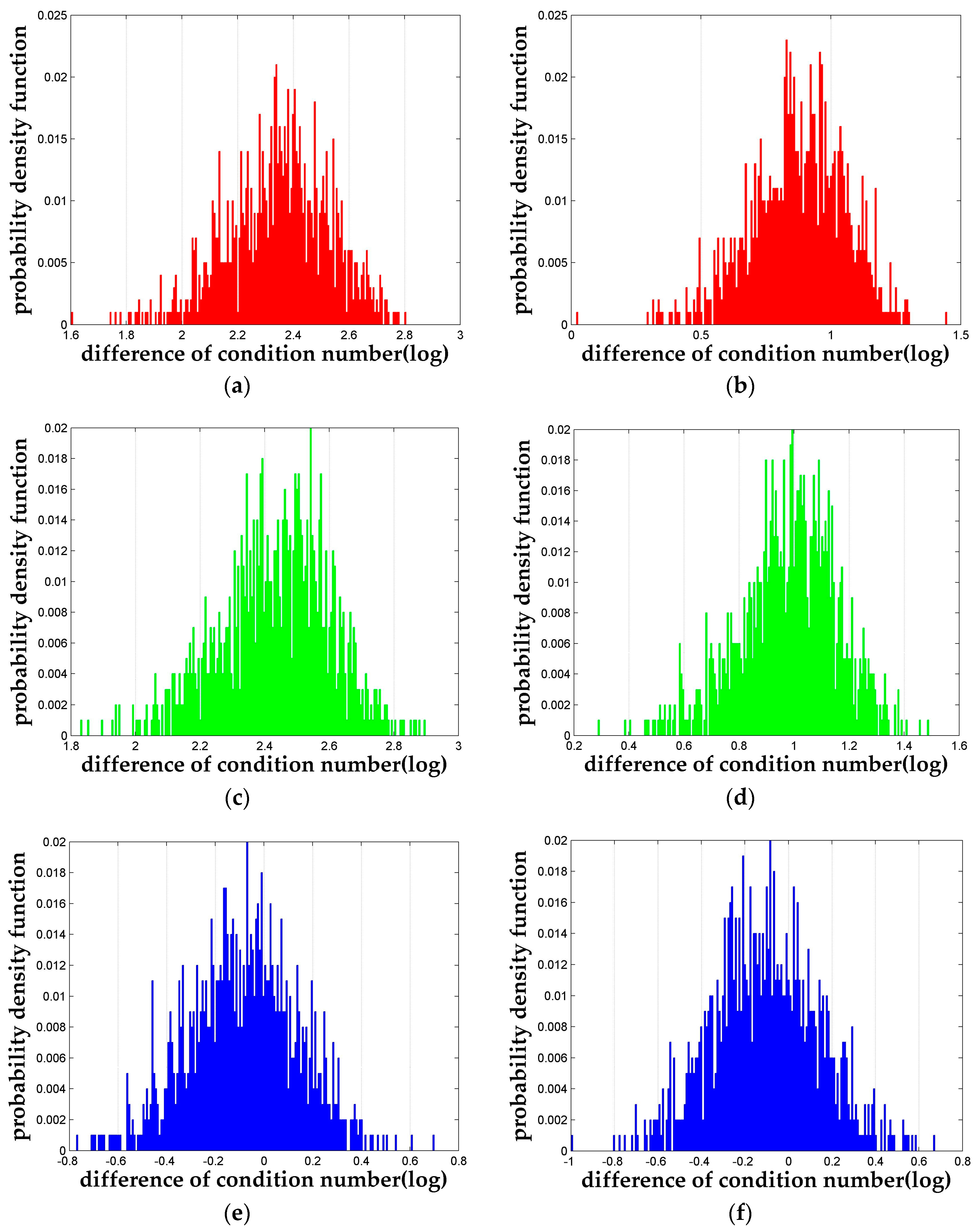
Firstly, we pick out a set of simulations where (for Case 1 only), and and the probability density function of the is plotted in Figure 3. It can be seen clearly in Figure 3a,b () and Figure 3c,d () that both the LLL reduction algorithm and the n-LLL reduction algorithm are able to reduce the condition number significantly. Furthermore, Figure 3e,f shows the difference between the two algorithms , which proves the 4-LLL reduction algorithm has larger probability to perform better than the original LLL reduction. Statistically, among the 1000 independent runs of this particular simulation setting, 64.7% results of the 4-LLL is better than that of the LLL with a maximum improvement factor of 5.85. And the average improvement is about 39%. It should be pointed out that for all the simulation settings mentioned above, the conclusion showed in Figure 3 holds in general.
In Section 3.2, inequality (28) implies that the lower bound of the reduction quality (the orthogonality of the coefficient matrix) improves as the parameter n increases. To prove this conclusion, we take for example and let the parameter n vary from 4 to 20. The results shown in Figure 4 is not as expected and an upper limit shows up for the as the n increases. And the condition number of the output matrix changes no more after n reaches a certain number. The explanation for this phenomenon is that the column vectors in cannot become “more ordered” to improve the orthogonality anymore at this point. However, Figure 4 still shows that (the original LLL) is generally not this upper limit and there is space to improve reduction performance by increasing the parameter n.
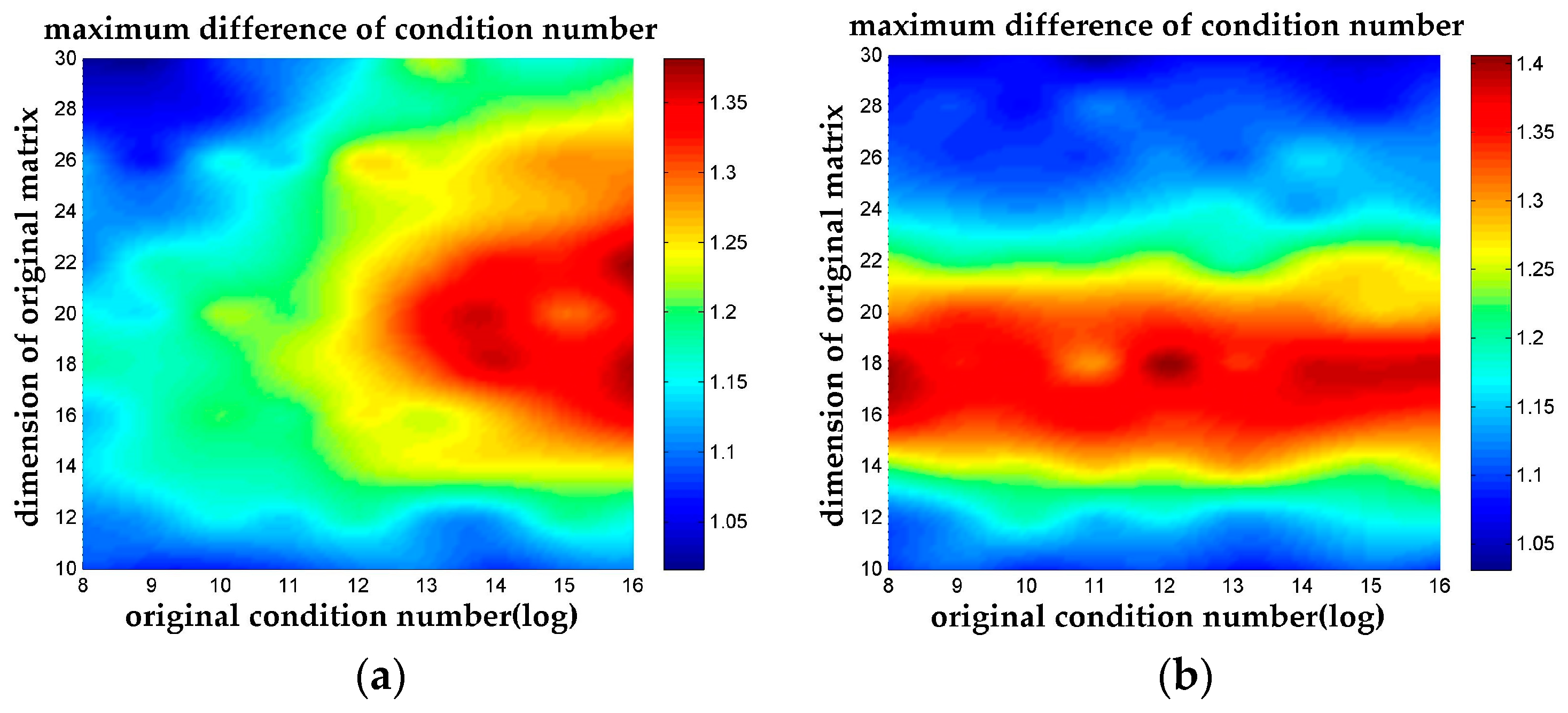
This can be clearly seen in the thermodynamic diagram Figure 5, where the temperature denotes . The highest temperature shows up when the dimension of the coefficient matrix is around 20 with a relatively high for Case 1, which indicates that the n-LLL reduction algorithm maximum its performance in that area. And for Case 2, the highest temperature also shows up around the dimension of 18 to 20. However, the difference between LLL and n-LLL becomes less significant when dealing with matrixes with higher dimension but lower condition number.
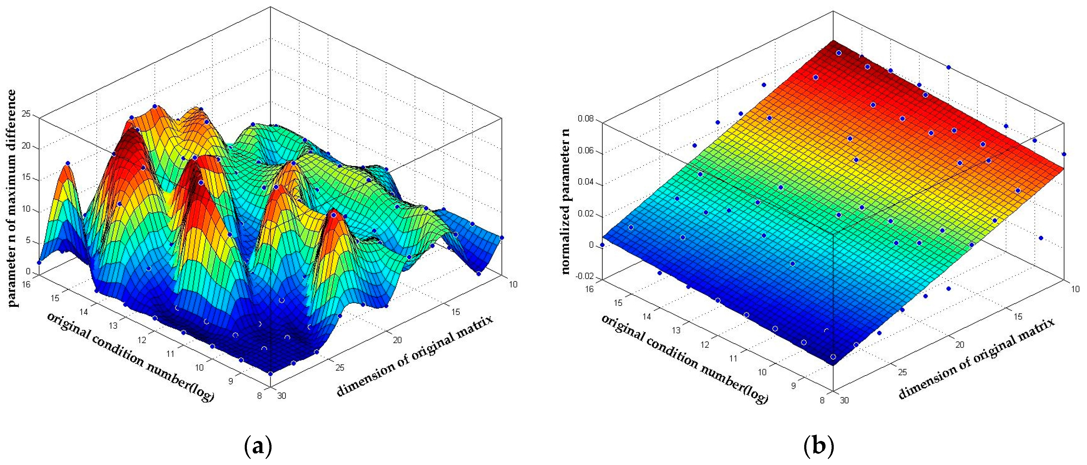
As can be seen later in Section 4.3.2, setting a higher parameter n always results in a longer reduction time. Thus, finding an optimized n to balance the performance and the reduction time is important. We analyzed the simulation results deeply and found that parameter n is relevant to the square of the dimension. We give out the fit result based on our simulation in Figure 6 and (43). The goodness of the first order polynomial surface fitting in Figure 6b reaches 0.6851, which means it can be taken as an empirical reference formula within the simulation setting range.
4.3.2. Complexity
In order to evaluate the effect of pivoted reflection, we compared the n-LLL reduction without pivoted reflection (PR), the n-LLL reduction with pivoted reflection and the original LLL reduction algorithm. The simulation is performed on an E5-2650 CPU which makes the executing time is relatively short. Thus, matrixes with high dimension and high condition number are chosen in this simulation to obtain more accurate time measurements. 1000 independent runs are performed for 30-dimensional matrixes with condition number range from to . And to evaluate the worst case of the n-LLL reduction algorithm, parameter n is fixed to 30 accordingly. Table 1 shows the simulation results, indicating that the pivoted reflection is very effective on improving the efficiency of the algorithm.
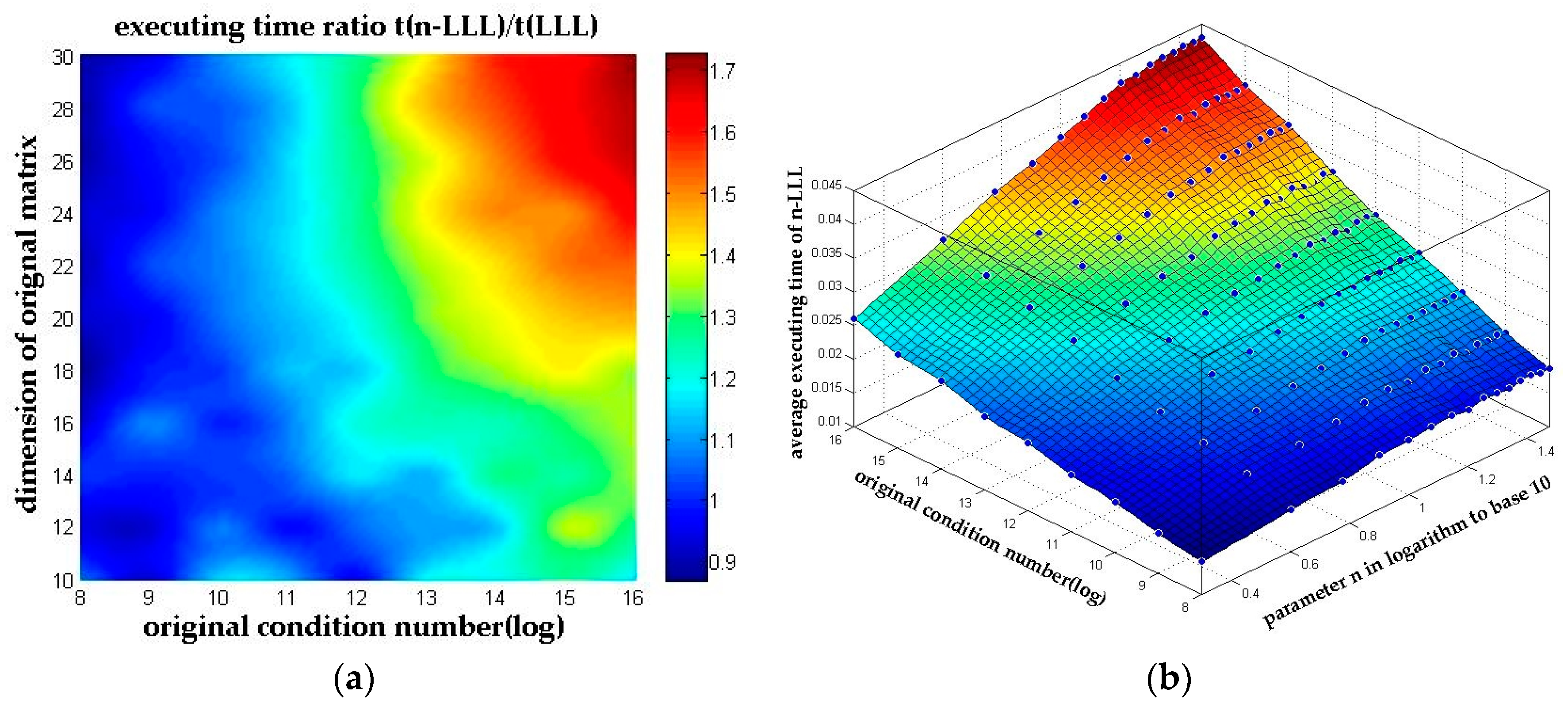
The conclusion is obvious that the pivoted reflection can reduce the reduction time by up to 57% and it is also clear that the n-LLL reduction algorithm with pivoted reflection causes no significant rise on the total reduction time compared with the original LLL reduction. And in the worst case scenario of all our simulations, the n-LLL reduction algorithm consumes no more than 1.72 times of the original LLL reduction time, which can also be observed in Figure 7a.
Take another look at the results in Figure 7a in a different angle where the parameter n is present in logarithm to base 10. The executing time in Figure 7b shows great linearity to the logarithm of parameter n, which meets the conclusion presented in Section 3.2.2 well.
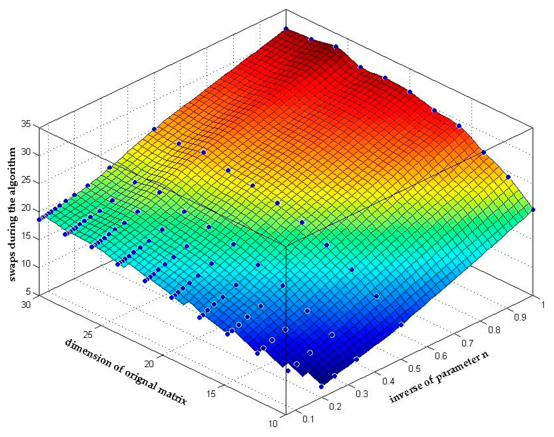
Figure 8 shows the relationship between the matrix dimension, the inverse of parameter n and the average number of swaps in the reduction process. As we analyzed in Section 3.2.2, (39) shows that the number of swaps will actually decline with the increase of parameter n as long as both the dimension and the condition number of the original matrix is determined. And this conclusion can be clearly seen in Figure 8 that the number of swaps declines by n times.
5. Conclusions
This paper has presented a new kind of lattice reduction algorithm motivated by the original LLL reduction. In order to put more emphasize on the order of the basis vectors, the Lovász condition is further strengthened, expanding the 2-dimensional local optimization to n-dimensional global optimization. The pivoted reflection method based on the Householder transformation and QR decomposition is added to the algorithm in order to reduce the additional computational effort brought by the extra vector swaps.
By utilizing the Hadamard Inequality and the orthogonality defect factor, the relation between the n parameter of n-LLL and the reduction quality is illustrated. Analysis shows that with the increase of the parameter n, the basis vectors will become more orthogonal or at least its orthogonality defect factor will have a smaller lower bound. The complexity of the n-LLL algorithm is estimated afterwards, which shows the n-LLL algorithm consumes more elementary steps than the original LLL with . However, the analysis also proves that the n-LLL algorithm still remains a polynomial-time algorithm.
In the numerical simulation, two basic cases are covered to mimic the features of GNSS double-difference carrier-phase measurements. The simulation results show that the reduction quality of n-LLL algorithm is better than the original LLL reduction algorithm, especially for highly ill-conditioned matrixes. However, with the increase of the parameter n, a certain upper bound of the reduction quality of n-LLL is found during the simulation. At this certain point, the effect of permutation reaches its limit and further permutation will not significantly affect the reduction quality. In this case, a first-order surface fit is given to estimate this certain parameter n.
In order to evaluate the effect of pivoted reflection, the n-LLL reduction with and without pivoted reflection as well as the original LLL reduction are compared. The results clearly show the power of pivoted reflection, especially for matrix with relatively low condition number. And in the worst case scenario of all our simulation, the pivoted reflection ensures the n-LLL reduction algorithm consumes no more than 1.72 times of the original LLL reduction executing time.
Both the analysis and the simulation results have shown that the n-LLL algorithm is better than the original LLL reduction algorithm, especially for highly ill-conditioned matrixes. And the increase of the total reduction time is fairly acceptable, which makes the n-LLL a new practical algorithm for lattice basis reduction.
Acknowledgments
The work is supported by the National Key Research and Development Program of China (No. 2016YFB0502001) and National Natural Science Foundation of China (No. 61372110).
Author Contributions
Zhongliang Deng proposed the general idea of the n-LLL reduction and pointed out the importance of the order of basis vectors; Di Zhu designed the algorithm, added pivoted reflection into the algorithm, performed the analysis and simulation and wrote the paper; Lu Yin helped to enrich the simulation results and to revise the paper.
Conflicts of Interest
The authors declare no conflict of interest.
References
- Provenzano, J.P.; Masson, A.; Journo, S.; Laramas, C.; Damidaux, J.I.; Zwolska, F. Implementation of a european infrastructure for satellite navigation: From system design to advanced technology evaluation. Int. J. Satell. Commun. Netw. 2015, 18, 223–242. [Google Scholar] [CrossRef]
- Dow, J.M.; Neilan, R.E.; Rizos, C. The international GNSS service in a changing landscape of global navigation satellite systems. J. Geodesy 2009, 83, 191–198. [Google Scholar] [CrossRef]
- Gerke, M.; Przybilla, H. Accuracy analysis of photogrammetric UAV image blocks: Influence of onboard RTK-GNSS and cross flight patterns. Photogramm. Fernerkund. Geoinf. 2016, 2016, 17–30. [Google Scholar] [CrossRef]
- Tahar, K.N.; Ahmad, A.; Wan, A.A.W.M.A.; Wan, M.N.W.M. Unmanned aerial vehicle photogrammetric results using different real time kinematic global positioning system approaches. In Lecture Notes in Geoinformation & Cartography; Springer: Berlin/Heidelberg, Germany, 2013; pp. 123–134. [Google Scholar]
- Woo, H.J.; Yoon, B.J.; Cho, B.G.; Kim, J.H. Research into navigation algorithm for unmanned ground vehicle using real time kinemtatic (RTK)-GPS. In Proceedings of the 2009 ICCAS-SICE, Fukuoka, Japan, 18–21 August 2009; pp. 2425–2428. [Google Scholar]
- Hatch, R. Instantaneous Ambiguity Resolution; Springer: New York, NY, USA, 1991. [Google Scholar]
- Forssell, B.; Martinneira, M.; Harrisz, R.A. Carrier phase ambiguity resolution in GNSS-2. In Proceedings of the 10th International Technical Meeting of the Satellite Division of The Institute of Navigation (ION GPS 1997), Kansas City, MO, USA, 16–19 September 1997; pp. 1727–1736. [Google Scholar]
- Teunissen, P.J.G. The least-squares ambiguity decorrelation adjustment: A method for fast GPS integer ambiguity estimation. J. Geodesy 1995, 70, 65–82. [Google Scholar] [CrossRef]
- Teunissen, P.J.G. Least-Squares Estimation of the Integer GPS Ambiguities. Invited lecture, Section IV “Theory and Methodology”. In Proceedings of the General Meeting of the International Association of Geodesy, Beijing, China, August 1993. [Google Scholar]
- Xu, P. Random simulation and gps decorrelation. J. Geodesy 2001, 75, 408–423. [Google Scholar] [CrossRef]
- Chang, X.W.; Yang, X.; Zhou, T. MLAMBDA: A modified LAMBDA method for integer least-squares estimation. J. Geodesy 2005, 79, 552–565. [Google Scholar] [CrossRef]
- Xu, P. Parallel cholesky-based reduction for the weighted integer least squares problem. J. Geodesy 2012, 86, 35–52. [Google Scholar] [CrossRef] [Green Version]
- Hassibi, A.; Boyd, S. Integer parameter estimation in linear models with applications to GPS. IEEE Trans. Signal Process. 1998, 46, 2938–2952. [Google Scholar] [CrossRef]
- Lenstra, A.K.; Lenstra, H.W.; Lovász, L. Factoring polynomials with rational coefficients. Math. Ann. 1982, 261, 515–534. [Google Scholar] [CrossRef]
- Wen, J.; Chang, X.W. GfcLLL: A greedy selection-based approach for fixed-complexity LLL Reduction. IEEE Commun. Lett. 2017, 21, 1965–1968. [Google Scholar] [CrossRef]
- Taherzadeh, M.; Mobasher, A.; Khandani, A.K. LLL reduction achieves the receive diversity in MIMO decoding. IEEE Trans. Inf. Theory 2007, 53, 4801–4805. [Google Scholar] [CrossRef]
- Ying, H.G.; Cong, L.; Mow, W.H. Complex lattice reduction algorithm for low-complexity MIMO detection. IEEE Trans. Signal Process. 2006, 5, 2701–2710. [Google Scholar]
- Grafarend, E.W. Mixed integer-real valued adjustment (IRA) problems: GPS initial cycle ambiguity resolution by means of the LLL algorithm. GPS Solut. 2000, 4, 31–44. [Google Scholar] [CrossRef]
- Nguên, P.Q.; Stehlé, D. Floating-Point LLL Revisited; Springer: Berlin/Heidelberg, Germany, 2005; pp. 215–233. [Google Scholar]
- Schnorr, C.P.; Euchner, M. Lattice basis reduction: Improved practical algorithms and solving subset sum problems. Math. Program. 1994, 66, 181–199. [Google Scholar] [CrossRef]
- Schnorr, C.P. A hierarchy of polynomial time basis reduction algorithms. Theor. Comput. Sci. 1987, 53, 375–386. [Google Scholar] [CrossRef]
- Fontein, F.; Schneider, M.; Wagner, U. PotLLL: A polynomial time version of LLL with deep insertions. Des. Codes Cryptogr. 2014, 73, 355–368. [Google Scholar] [CrossRef]
- Babai, L. On Lovász’ lattice reduction and the nearest lattice point problem. In Proceedings of the STACS 85 Symposium on Theoretical Aspects of Computer Science, Saarbrücken, Germany, 3–5 January 1985; pp. 13–20. [Google Scholar]
- Wübben, D.; Bohnke, R.; KüHn, V.; Kammeyer, K.D. MMSE extension of V-BLAST based on sorted QR decomposition. In Proceedings of the Vehicular Technology Conference, Orlando, FL, USA, 6–9 October 2003; Volume 501, pp. 508–512. [Google Scholar]
- Vetter, H.; Ponnampalam, V.; Sandell, M.; Hoeher, P.A. Fixed complexity LLL algorithm. IEEE Trans. Signal Process. 2009, 57, 1634–1637. [Google Scholar] [CrossRef]
- Borno, M.A.; Chang, X.W.; Xie, X.H. On “decorrelation” in solving integer least-squares problems for ambiguity determination. Emp. Surv. Rev. 2014, 46, 37–49. [Google Scholar] [CrossRef]
- Xu, P. Voronoi cells, probabilistic bounds, and hypothesis testing in mixed integer linear models. IEEE Trans. Inf. Theory 2006, 52, 3122–3138. [Google Scholar] [CrossRef]
- Jonge, P.P.D.; Tiberius, C. On the spectrum of the GPS DD-ambiguities. In Proceedings of the 7th International Technical Meeting of the Satellite Division of the Institute of Navigation, Salt Lake City, UT, USA, 20–23 September 1994. [Google Scholar]
- Teunissen, P.J.G.; Jonge, P.P.D.; Tiberius, C. The least-squares ambiguity decorrelation adjustment: Its performance on short GPS baselines and short observation spans. J. Geodesy 1997, 71, 589–602. [Google Scholar] [CrossRef]
Figure 1.
Illustration of “Bad” and “Good” lattice basis.

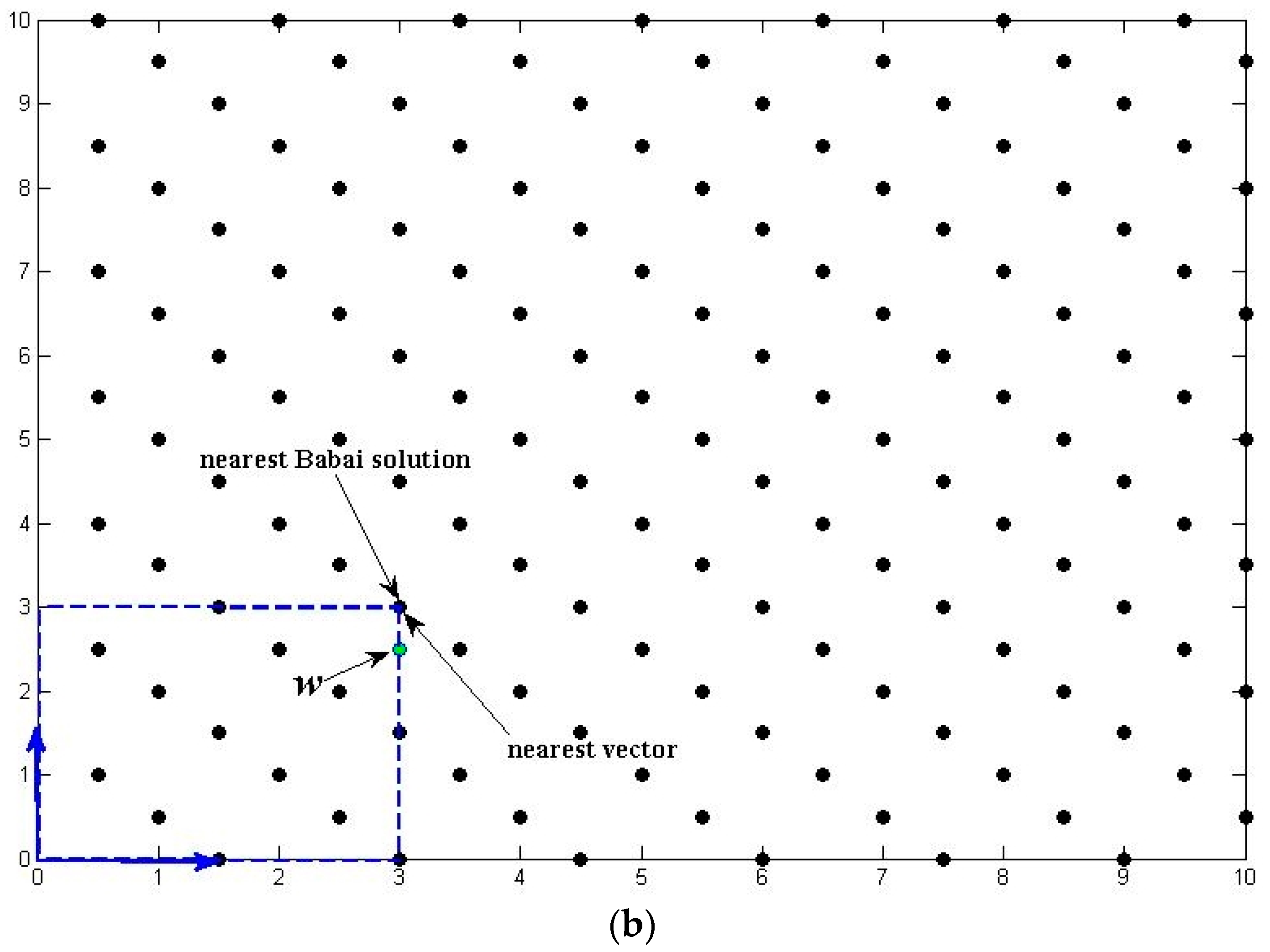
Figure 2.
The effect of lattice reduction on the searching space.
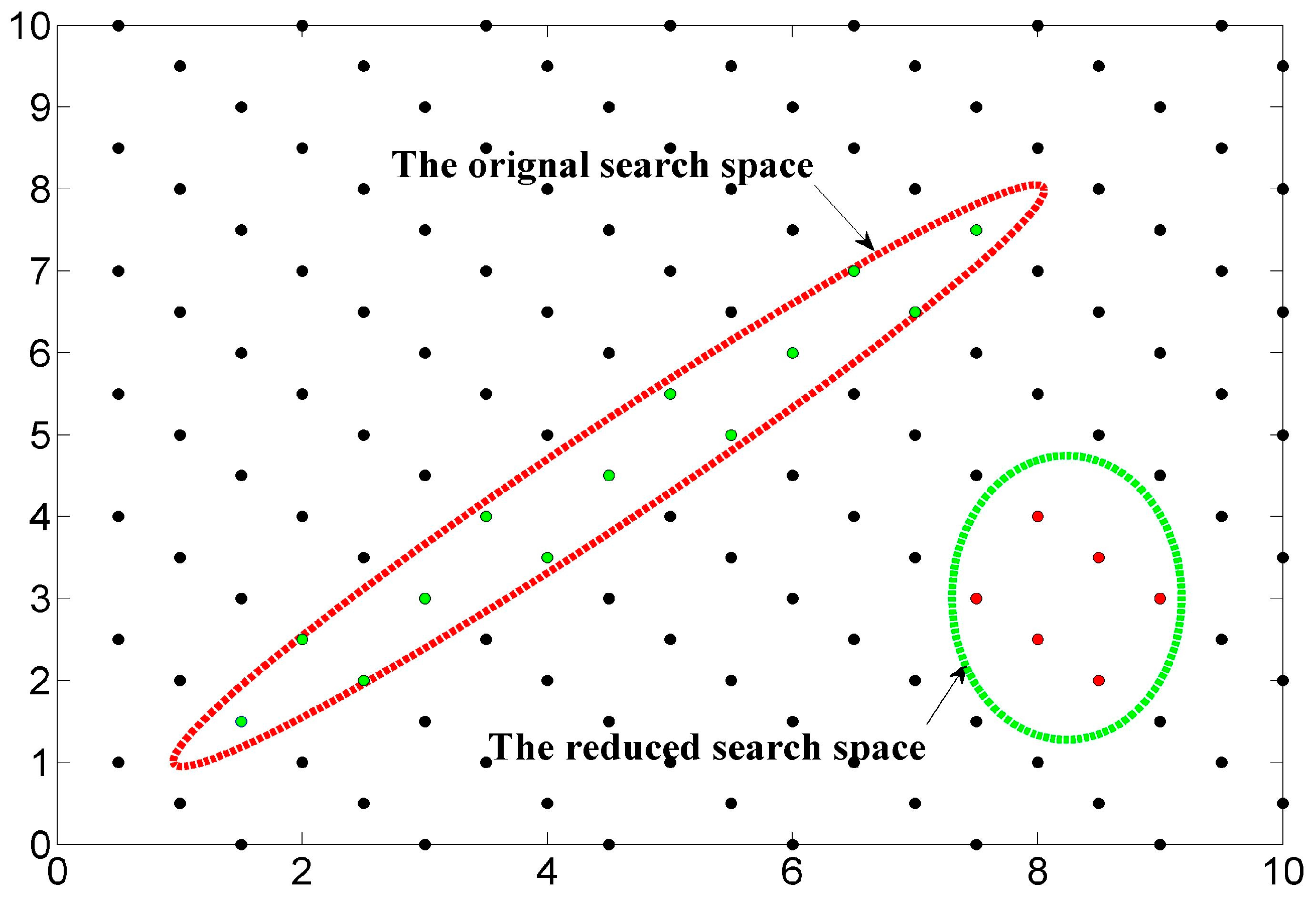
Figure 3.
The probability density functions of the differences of condition numbers in logarithm to base 10. (a) dκ between the original matrix and LLL reduced matrix for κorig = 212 of Case 1; (b) dκ between the original matrix and LLL reduced matrix for Case 2; (c) dκ between the original matrix and 4-LLL reduced matrix for κorig = 212 of Case 1; (d) dκ between the original matrix and 4-LLL reduced matrix for Case 2; (e) dκ between the LLL reduced matrix and 4-LLL reduced matrix for κorig = 212 of Case 1; (f) dκ between the LLL reduced matrix and 4-LLL reduced matrix for Case 2.

Figure 4.
Normalized difference of condition numbers. The differences of condition number between n-LLL and the original LLL are normalized and plotted altogether with m range from 18 to 24. (a) The normalized difference of condition number for κorig = 214 of Case 1; (b) The normalized difference of condition number of Case 2.

Figure 5.
The maximum difference of condition numbers. The max value of the difference of condition number between n-LLL and LLL among all possible n parameter is plotted in the thermodynamic diagram. (a) The maximum difference of condition numbers for Case 1; (b) The maximum difference of condition numbers for Case 2.

Figure 6.
The parameter n with the best reduction quality. The corresponding parameter n of the max difference of condition numbers in Figure 5a. (a) The distribution of parameter n with the best reduction quality; (b) The 1st order fit of normalized parameter n/m2.
Figure 6.
The parameter n with the best reduction quality. The corresponding parameter n of the max difference of condition numbers in Figure 5a. (a) The distribution of parameter n with the best reduction quality; (b) The 1st order fit of normalized parameter n/m2.

Figure 7.
The executing time of n-LLL. (a) The executing time ratio between n-LLL and the original LLL algorithm; (b) The average executing time of n-LLL with parameter n presented in logarithm to base 10.
Figure 7.
The executing time of n-LLL. (a) The executing time ratio between n-LLL and the original LLL algorithm; (b) The average executing time of n-LLL with parameter n presented in logarithm to base 10.

Figure 8.
Number of swaps during the n-LLL algorithm.

Table 1.
The executing time of n-LLL reduction and LLL reduction.
| Condition Number | n-LLL without PR | n-LLL with PR | Original LLL |
|---|---|---|---|
| 536 ms | 230 ms | 217 ms | |
| 561 ms | 251 ms | 224 ms | |
| 595 ms | 286 ms | 222 ms | |
| 628 ms | 316 ms | 220 ms | |
| 651 ms | 341 ms | 222 ms | |
| 672 ms | 369 ms | 235 ms | |
| 714 ms | 412 ms | 239 ms |
© 2018 by the authors. Licensee MDPI, Basel, Switzerland. This article is an open access article distributed under the terms and conditions of the Creative Commons Attribution (CC BY) license (http://creativecommons.org/licenses/by/4.0/).
Share and Cite
MDPI and ACS Style
Deng, Z.; Zhu, D.; Yin, L. N-Dimensional LLL Reduction Algorithm with Pivoted Reflection. Sensors 2018, 18, 283. https://doi.org/10.3390/s18010283
AMA Style
Deng Z, Zhu D, Yin L. N-Dimensional LLL Reduction Algorithm with Pivoted Reflection. Sensors. 2018; 18(1):283. https://doi.org/10.3390/s18010283
Chicago/Turabian StyleDeng, Zhongliang, Di Zhu, and Lu Yin. 2018. "N-Dimensional LLL Reduction Algorithm with Pivoted Reflection" Sensors 18, no. 1: 283. https://doi.org/10.3390/s18010283
Note that from the first issue of 2016, this journal uses article numbers instead of page numbers. See further details here.