Vehicle Speed and Length Estimation Using Data from Two Anisotropic Magneto-Resistive (AMR) Sensors


 ,
,
Abstract
:1. Introduction
2. Related Works
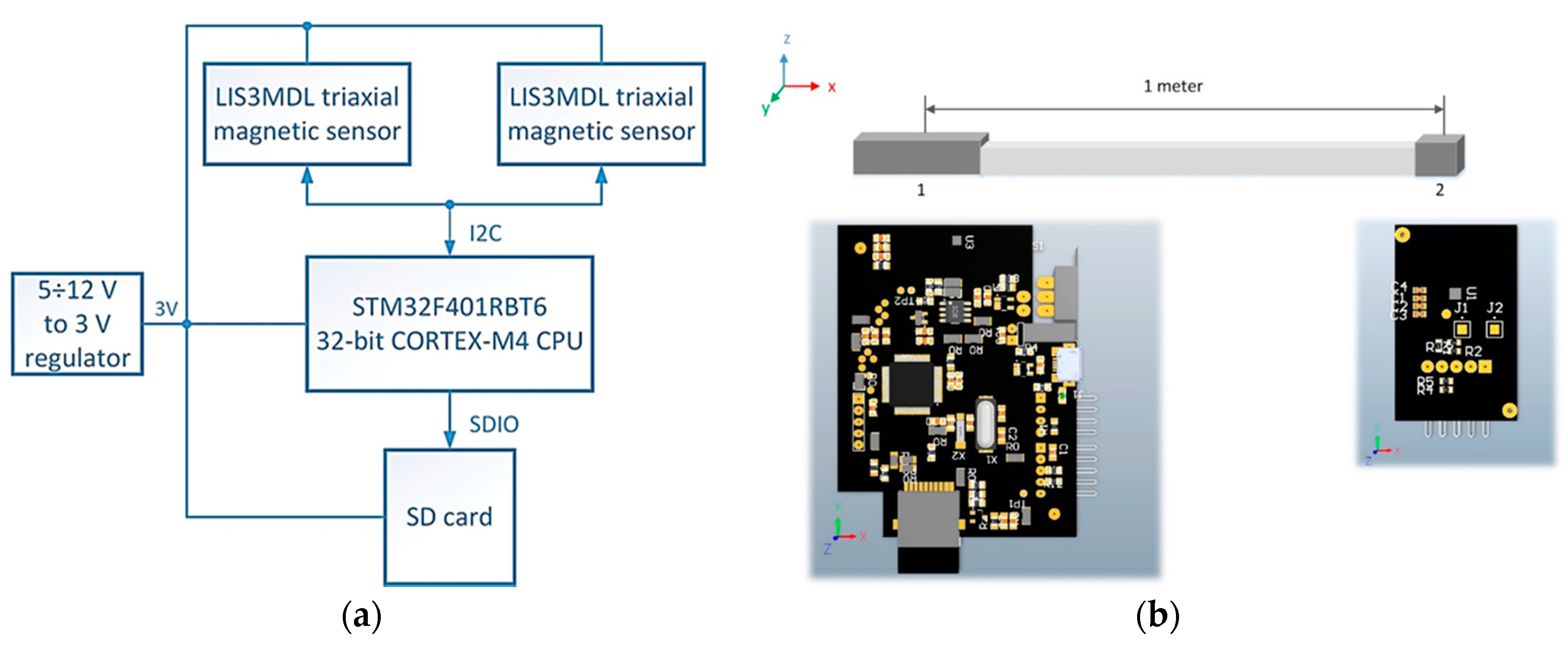
3. Measuring System
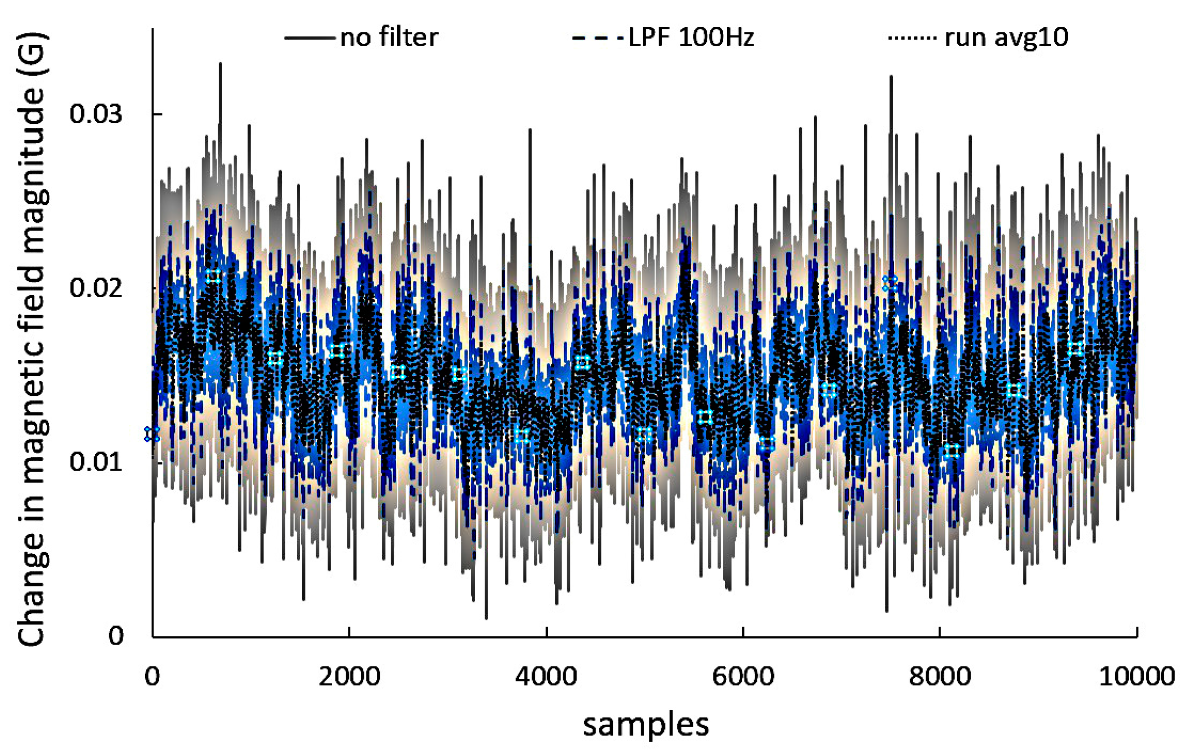
4. Noise in Signals
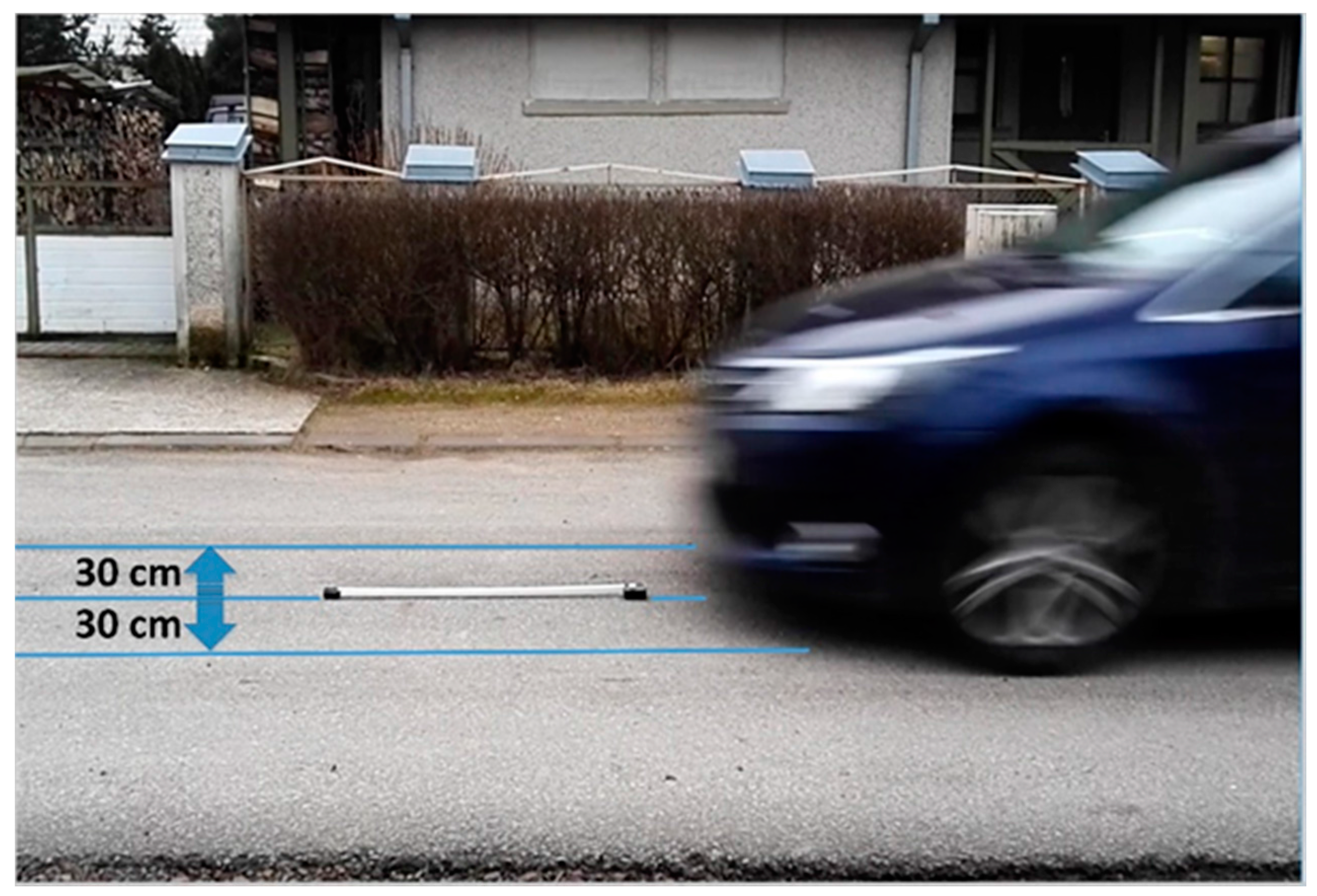
5. Experiments
- from the North to the South (N-S) and from the South to the North (S-N)
- from the West to the East (W-E) and from the East to the West (E-W)
6. Speed and Length Measurement Evaluation on the Basis of the Magnitude Signal and Z-Component Signal of the Magnetic Field
6.1. Speed Measurement
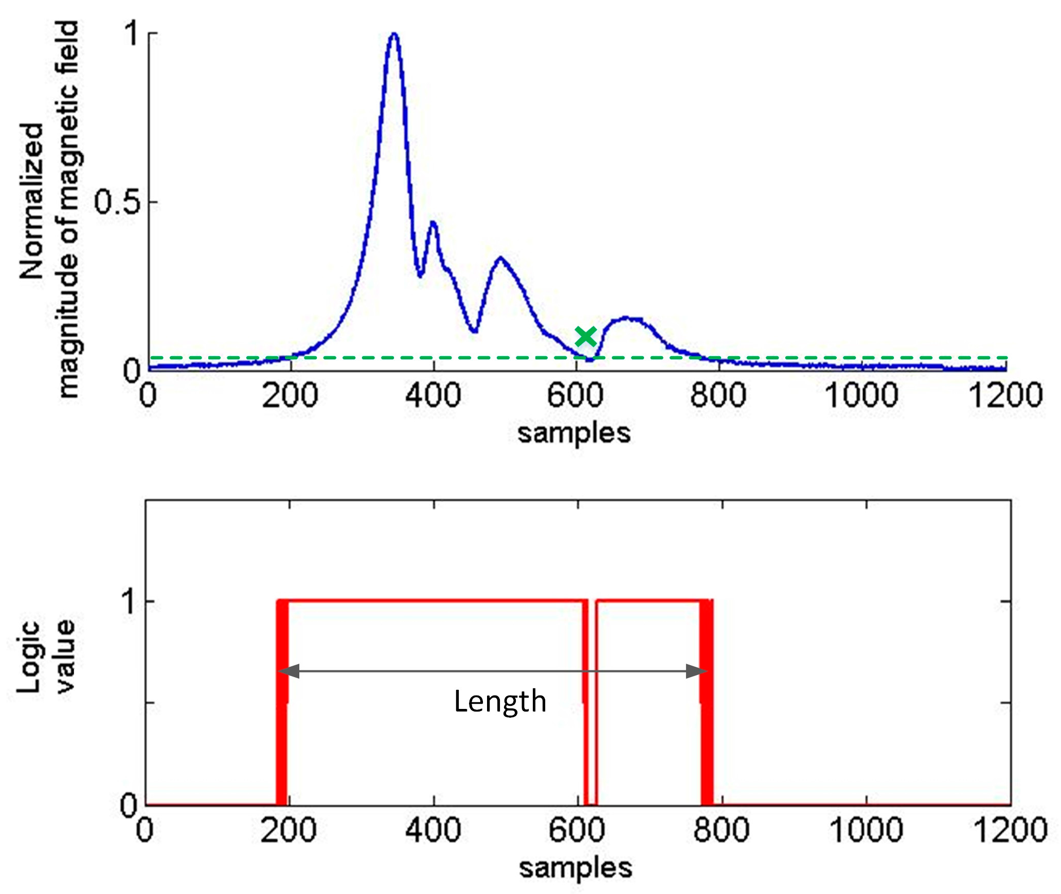
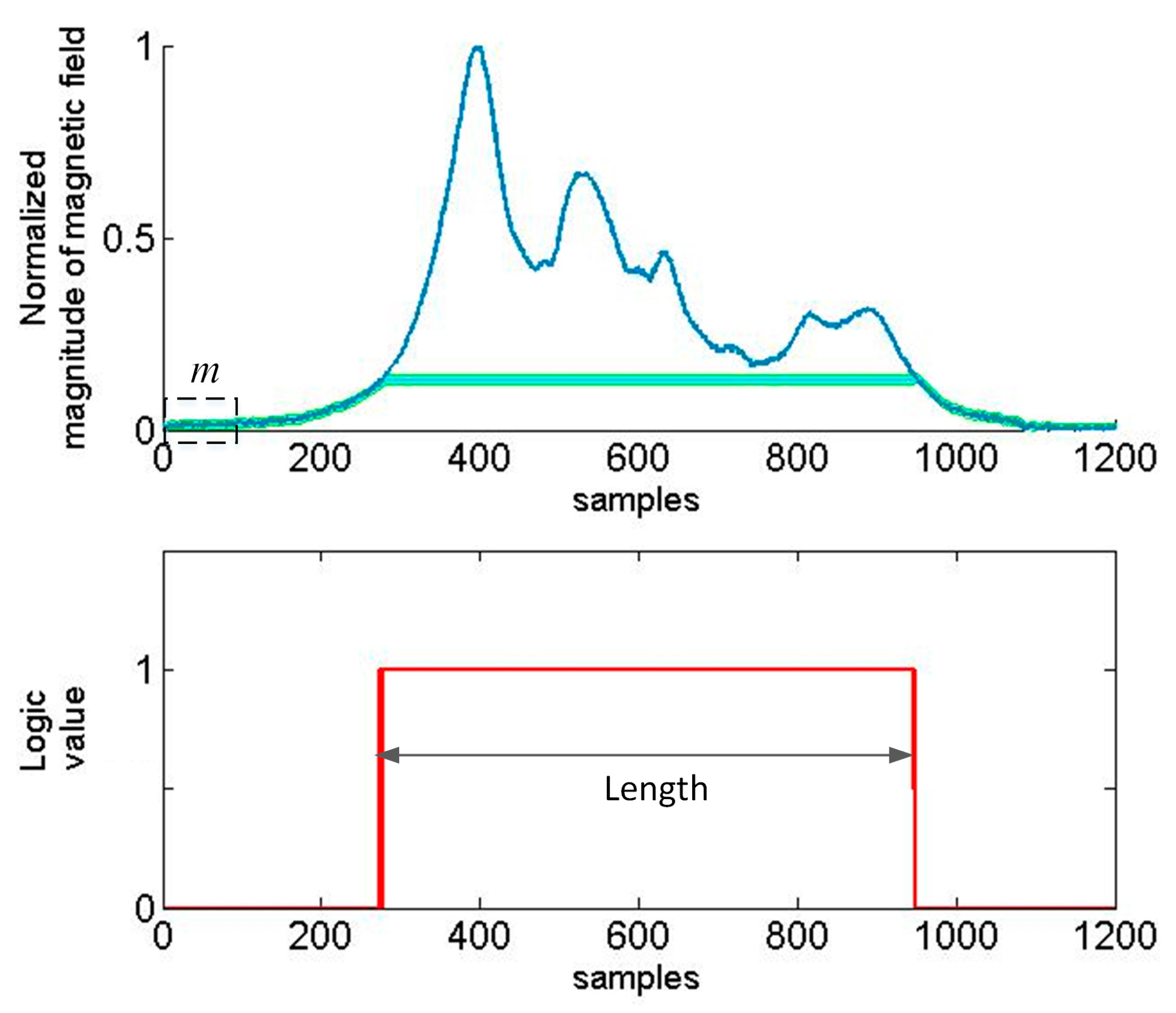
6.2. The Simple Threshold-Based Detection Method (Method 1)
6.3. Threshold Method Based on the Moving Average and kSD (Method 2)
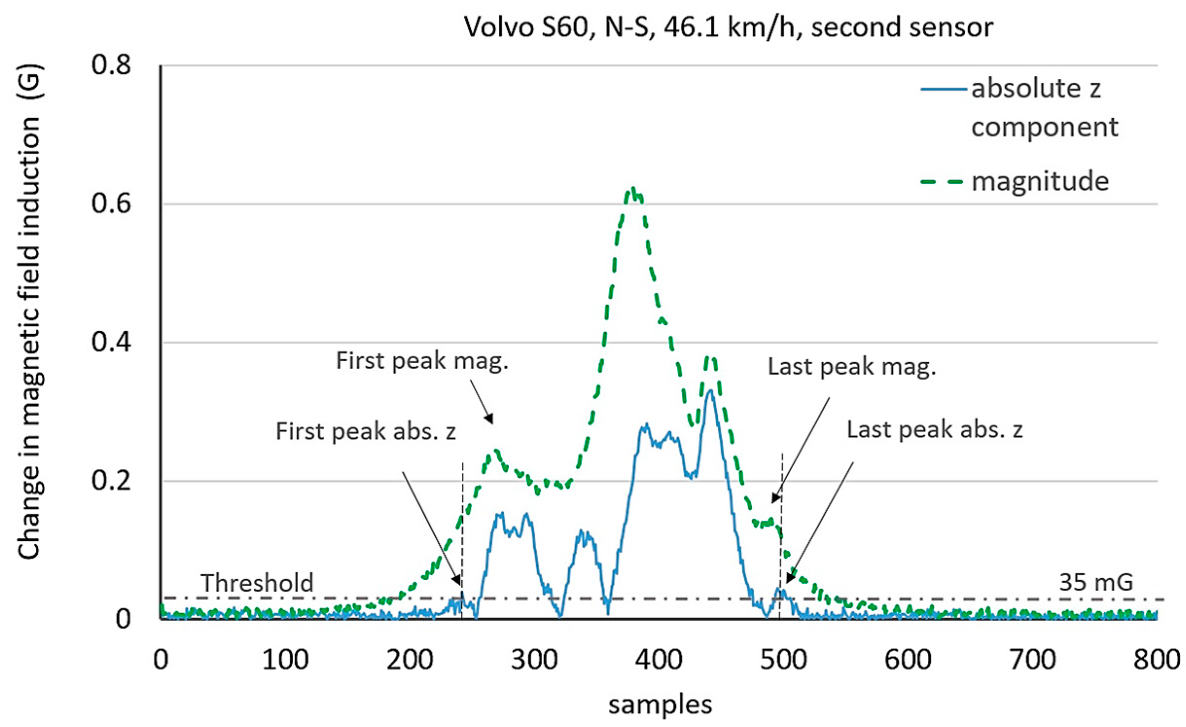
6.4. Two-Extreme-Peak Detection (Method 3)
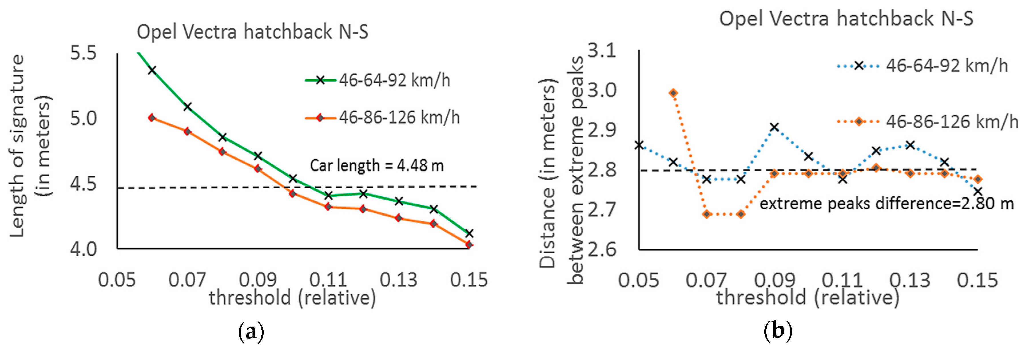
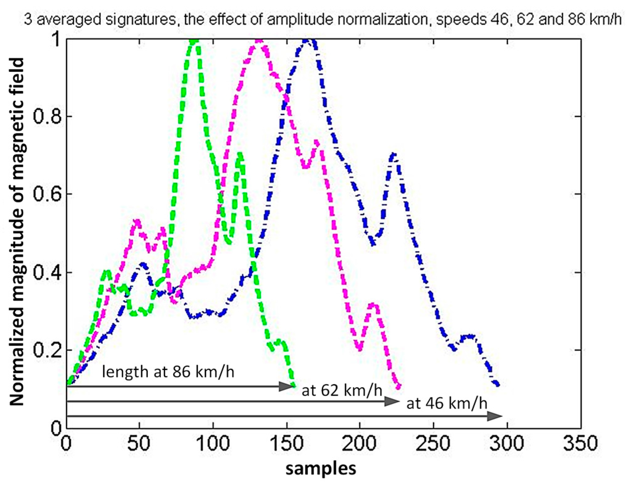
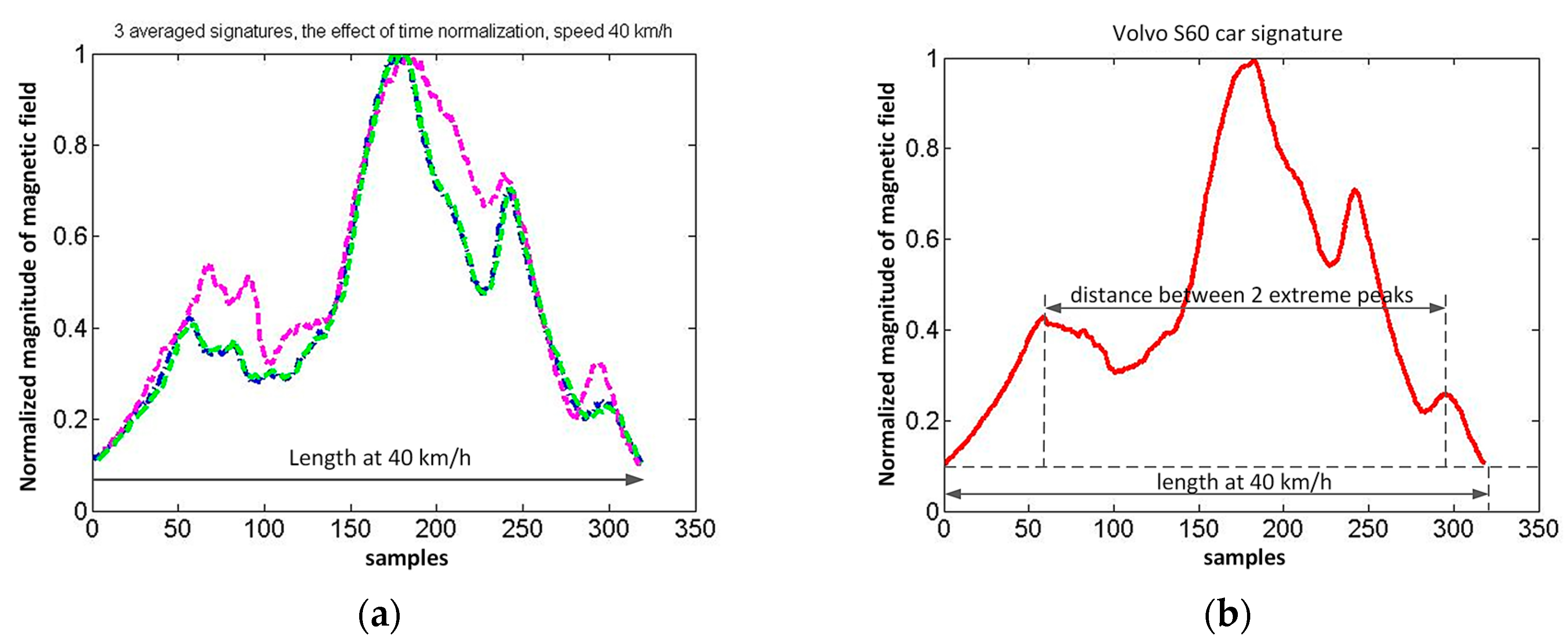
6.5. Method Based on the Amplitude and Time Normalization Using Linear Extrapolation or Interpolation (Method 4)
7. Results
8. Conclusions
Author Contributions
Conflicts of Interest
References
- Coifman, B.; Kim, S. Speed estimation and length based vehicle classification from freeway single-loop detectors. Transp. Res. Part C Emerg. Technol. 2009, 17, 349–364. [Google Scholar] [CrossRef]
- Llorca, D.F.; Salinas, C.; Jiménez, M.; Parra, I.; Morcillo, A.G.; Izquierdo, R.; Lorenzo, J.; Sotelo, M.A. Two-camera based accurate vehicle speed measurement using average speed at a fixed point. In Proceedings of the IEEE 19th International Conference on Intelligent Transportation Systems (ITSC), Rio de Janeiro, Brazil, 1–4 November 2016; pp. 2533–2538. [Google Scholar]
- Placentino, F.; Alimenti, F.; Battistini, A.; Bernardini, W.; Mezzanotte, P.; Palazzari, V.; Leone, S.; Scarponi, A.; Porzi, N.; Comez, M.; et al. Measurements of length and velocity of vehicles with a low cost sensor radar doppler operating at 24GHz. In Proceedings of the 2nd IEEE International Workshop on Advances in Sensors and Interfaces (IWASI 2007), Bari, Italy, 26–27 June 2007; pp. 1–5. [Google Scholar]
- Iwasaki, Y. A method of real-time moving vehicle detection for bad environments using infrared thermal images. In Innovations and Advanced Techniques in Systems, Computing Sciences and Software Engineering; Elleithy, K., Ed.; Springer: Dordrecht, The Netherlands, 2008; pp. 43–46. [Google Scholar]
- Velisavljevic, V.; Cano, E.; Dyo, V.; Allen, B. Wireless magnetic sensor network for road traffic monitoring and vehicle classification. Transp. Telecommun. 2016, 17, 274–288. [Google Scholar] [CrossRef]
- Vala, D. Using spread spectrum for AMR magnetic sensor. In Proceedings of the Photonics Applications in Astronomy, Communications, Industry, and High-Energy Physics Experiments 2016, Wilga, Poland, 29 May–6 June 2016. [Google Scholar] [CrossRef]
- Ripka, P.; Janosek, M. Advances in magnetic field sensors. IEEE Sens. J. 2010, 10, 1108–1116. [Google Scholar] [CrossRef]
- De Angelis, G.; De Angelis, A.; Pasku, V.; Moschitta, A.; Carbone, P. A simple magnetic signature vehicles detection and classification system for smart cities. In Proceedings of the 2016 IEEE International Symposium on Systems Engineering (ISSE), Edinburgh, UK, 3–5 October 2016; pp. 1–6. [Google Scholar]
- Kaewkamnerd, S.; Pongthornseri, R.; Chinrungrueng, J.; Silawan, T. Automatic vehicle classification using wireless magnetic sensor. In Proceedings of the 5th IEEE International Workshop on Intelligent Data Acquisition and Advanced Computing Systems: Technology and Applications (IDAACS), Rende, Italy, 21–23 September 2009; pp. 420–424. [Google Scholar]
- Jolevski, I.; Markoski, A.; Pasic, R. Smart vehicle sensing and classification node with energy-aware vehicle classification algorithm. In Proceedings of the 33rd International Conference on Information Technology Interfaces (ITI), Dubrovnik, Croatia, 27–30 June 2011; pp. 409–414. [Google Scholar]
- Taghvaeeyan, S.; Rajamani, R. Portable roadside sensors for vehicle counting, classification, and speed measurement. IEEE Trans. Intell. Transp. Syst. 2014, 15, 73–83. [Google Scholar] [CrossRef]
- Markevicius, V.; Navikas, D.; Daubaras, A.; Cepenas, M.; Zilys, M.; Andriukaitis, D. Vehicle influence on the earth’s magnetic field changes. Elektron. Elektrotech. 2014, 20, 43–48. [Google Scholar] [CrossRef]
- Markevicius, V.; Navikas, D.; Zilys, M.; Andriukaitis, D.; Valinevicius, A.; Cepenas, M. Dynamic vehicle detection via the use of magnetic field sensors. Sensors 2016, 16, 78. [Google Scholar] [CrossRef] [PubMed]
- Haoui, A.; Kavaler, R.; Varalya, P. Wireless magnetic sensors for traffic surveillance. Transp. Res. Part C Emerg. Technol. 2008, 16, 294–306. [Google Scholar] [CrossRef]
- Zhu, H.; Yu, F. A cross-correlation technique for vehicle detections in wireless magnetic sensor network. IEEE Sens. J. 2016, 16, 4484–4494. [Google Scholar] [CrossRef]


| Direction N-S | Method 1 | Method 2 | Method 3 | |||
|---|---|---|---|---|---|---|
| Magnitude | abs z | Magnitude | abs z | Magnitude | abs z | |
| Opel Vectra (C) | car length 4.481 m, wheelbase 2.639 m, ground clearance 0.16 m | |||||
| speed 1 = 46.1 km/h | 5.117 | 4.116 | 5.233 | 5.299 | 2.917 | 3.000 |
| speed 2 = 64.3 km/h | 5.116 | 3.953 | 5.488 | 4.279 | 2.977 | 3.046 |
| speed 3 = 86.5 km/h | 5.125 | 3.899 | 5.062 | 3.900 | 2.937 | 3.033 |
| mean | 5.119 | 3.989 | 5.261 | 4.492 | 2.944 | 3.026 |
| Volvo S60 (C) | car length 4.577 m, wheelbase 2.715 m, ground clearance 0.13 m | |||||
| speed 1 = 46.1 km/h | 5.683 | 3.566 | 5.933 | 3.383 | 3.666 | 3.800 |
| speed 2 = 62.9 km/h | 5.477 | 3.773 | 5.772 | 3.273 | 3.659 | 4.182 |
| speed 3 = 86.5 km/h | 5.500 | 3.594 | 5.562 | 3.844 | 3.625 | 3.719 |
| mean | 5.553 | 3.641 | 5.756 | 3.513 | 3.650 | 3.900 |
| Direction E-W (Forward) Toyota Auris (C/S/N) | Method 1 | Method 2 | Method 3 | |||
| Magnitude | abs z | Magnitude | abs z | Magnitude | abs z | |
| speed 1 = 27.4 km/h (C) | 6.525 | 4.831 | 5.733 | 4.999 | 3.455 | 4.049 |
| speed 2 = 35.0 km/h (S) | 6.127 | 3.524 | 4.975 | 3.429 | 4.088 | 4.595 |
| speed 3 = 32.9 km/h (N) | 6.452 | 4.940 | 6.190 | 4.979 | 3.822 | 3.821 |
| Direction W-E (Reverse) Toyota Auris (C/S/N) | Method 1 | Method 2 | Method 3 | |||
| Magnitude | abs z | Magnitude | abs z | Magnitude | abs z | |
| speed 1 = 28.5 km/h (C) | 6.278 | 4.360 | 5.443 | 4.639 | 3.845 | 4.154 |
| speed 2 = 37.4 km/h (S) | 5.892 | 3.797 | 5.622 | 5.000 | 3.689 | 4.865 |
| speed 3 = 31.8 km/h (N) | 6.632 | 5.000 | 6.460 | 6.034 | 3.885 | 5.149 |
| Direction N-S Normalized Speed 4 = 40 km/h | Method 4 (Magnitude) | Method 4 (Magnitude) |
|---|---|---|
| Length of Signature (m) | Distance between Two Extreme Peaks (m) | |
| Opel Vectra (C) | car length 4.481 m, wheelbase 2.639 m, ground clearance 0.16 m | |
| threshold 0.10, speed 1–3: 46, 86, 126 km/h | 4.424 | 2.790 |
| threshold 0.10, speed 1–3: 46, 64, 92 km/h | 4.540 | 2.884 |
| Volvo S60 (C) | car length 4.577 m, wheelbase 2.715 m, ground clearance 0.13 m | |
| threshold 0.10, speed 1–3: 46, 62, 86 km/h | 4.597 | 3.412 |
| Car, Direction | Length (Met. 1) L1 | Length (Met. 3) L3 | Real Length RL | Ratio 1 RL/L1 | Ratio 3 L3/RL | Result (Ratio 3 = 0.75) | Error (Ratio 3 = 0.75) | Result (Ratio 1 = 0.75) | Error (Ratio 1 = 0.75) |
|---|---|---|---|---|---|---|---|---|---|
| m | m | m | - | - | m | % | m | % | |
| O. Vectra, N-S | 5.023 | 2.932 | 4.481 | 0.893 | 0.654 | 3.909 | 12.75 | 3.767 | 15.91 |
| O. Vectra, S-N | 6.168 | 3.269 | 4.481 | 0.727 | 0.730 | 4.358 | 2.72 | 4.626 | 3.26 |
| Volvo S60, N-S | 5.553 | 3.650 | 4.570 | 0.823 | 0.799 | 4.867 | 6.49 | 4.165 | 8.86 |
| T. Avensis, E-W | 6.887 | 4.153 | 4.765 | 0.693 | 0.872 | 5.537 | 16.21 | 5.165 | 8.40 |
| T. Avensis, W-E | 6.948 | 4.167 | 4.765 | 0.686 | 0.875 | 5.556 | 16.60 | 5.211 | 9.37 |
| S. Superb, E-W | 6.181 | 3.046 | 4.838 | 0.783 | 0.630 | 4.061 | 16.05 | 4.636 | 4.18 |
| Lexus RX, E-W | 6.385 | 4.366 | 4.770 | 0.747 | 0.915 | 5.821 | 22.04 | 4.789 | 0.39 |
© 2017 by the authors. Licensee MDPI, Basel, Switzerland. This article is an open access article distributed under the terms and conditions of the Creative Commons Attribution (CC BY) license (http://creativecommons.org/licenses/by/4.0/).
Share and Cite
Markevicius, V.; Navikas, D.; Idzkowski, A.; Valinevicius, A.; Zilys, M.; Andriukaitis, D. Vehicle Speed and Length Estimation Using Data from Two Anisotropic Magneto-Resistive (AMR) Sensors. Sensors 2017, 17, 1778. https://doi.org/10.3390/s17081778
Markevicius V, Navikas D, Idzkowski A, Valinevicius A, Zilys M, Andriukaitis D. Vehicle Speed and Length Estimation Using Data from Two Anisotropic Magneto-Resistive (AMR) Sensors. Sensors. 2017; 17(8):1778. https://doi.org/10.3390/s17081778
Chicago/Turabian StyleMarkevicius, Vytautas, Dangirutis Navikas, Adam Idzkowski, Algimantas Valinevicius, Mindaugas Zilys, and Darius Andriukaitis. 2017. "Vehicle Speed and Length Estimation Using Data from Two Anisotropic Magneto-Resistive (AMR) Sensors" Sensors 17, no. 8: 1778. https://doi.org/10.3390/s17081778