Performance Analysis of the Direct Position Determination Method in the Presence of Array Model Errors


1
National Digital Switching System Engineering & Technological Research Center, Zhengzhou 450002, China
2
Zhengzhou Information Science and Technology Institute, Zhengzhou 450002, China
*
Author to whom correspondence should be addressed.
Sensors 2017, 17(7), 1550; https://doi.org/10.3390/s17071550
Submission received: 8 May 2017
/
Revised: 22 June 2017
/
Accepted: 29 June 2017
/
Published: 2 July 2017
(This article belongs to the Special Issue Recent Advances in Array Signal Processing and Its Applications in IoT Security)
Abstract
:The direct position determination approach was recently presented as a promising technique for the localization of a transmitting source with accuracy higher than that of the conventional two-step localization method. In this paper, the theoretical performance of a direct position determination estimator proposed by Weiss is examined for situations in which the array model errors are present. Our study starts from a matrix eigen-perturbation result, which expresses the perturbation of eigenvalues as a function of the disturbance added to the Hermitian matrix. The first-order asymptotic expression of the positioning errors is presented, from which an analytical expression for the mean square error of the direct localization is available. Additionally, explicit formulas for computing the probabilities of a successful localization are deduced. Finally, Cramér–Rao bound expressions for the position estimation are derived for two cases: (1) array model errors are absent and (2) array model errors are present. The obtained Cramér-Rao bounds provide insights into the effects of the array model errors on the localization accuracy. Simulation results support and corroborate the theoretical developments made in this paper.
1. Introduction
The techniques of emitter localization using direction of arrival (DOA) measurements [1,2,3,4,5] play an important role in many areas, including vehicle navigation, localization and tracking of acoustic sources, and location services of satellite communications. In such localization systems, a single moving observer or multiple stationary observers are used to determinate the positions of the emitters. Generally, each observer is equipped with an antenna array for measuring the DOAs of the transmitted sources, and the emitter can then be located at the intersection of a set of lines of bearing [6,7,8]. The location procedure described above is typically called the two-step method. In the first step, the signal parameters (e.g., DOA [1,2,3,4,5], time difference of arrival (TDOA) [9,10], time of arrival (TOA) [11,12], frequency difference of arrival (FDOA) [13,14], frequency of arrival (FOA) [15], and received signal strength (RSS) [16,17]) are separately measured at several stations. In the second step, a central station uses the measurements to estimate the position coordinates of the sources. The two-step procedure is also known as the decentralized approach [18]. Note that although the two-step procedure is widely applied to the modern localization system, it is difficult to yield the optimal position estimate from the point of view of statistical characteristics. The reason is that the signal parameters are obtained by ignoring the constraint that all measurements must correspond to a common source position. As a result, information loss between the two steps is unavoidable. Although it can be proved by the extended invariance principle (EXIP) [19] that the two-step method provides an asymptotically efficient estimate under certain conditions, these requirements cannot be easily met in practical scenarios.
To improve the accuracy of two-step location methods, a promising technique, called the direct position determination (DPD) approach, is proposed over the past few years. DPD is a centralized and single-step estimation technique in which the estimator uses exactly the same data as classical two-step methods but searches for the source location directly. Generally, the DPD method outperforms conventional two-step methods under low-signal-to-noise conditions and when there are relatively few samples; moreover, it does not encounter the association problem. More importantly, the DPD technique can be applied to many wireless positioning systems. Specifically, the DPD method for locating a narrowband radio emitter based on a Doppler shift is presented in [20,21], and DPD methods for locating a wideband source based on a time delay metric are proposed in [22,23,24]. Furthermore, DPD estimators using both the Doppler frequency and time delay are developed in [25,26,27,28]. Note that in the DPD methods mentioned above, multiple platforms each equipped with a single-antenna receiver are used for position determination, and as a result, the DOA information of the impinging signals cannot be exploited. In [29], a DPD method based on multiple static stations each equipped with an antenna array is first proposed. In this single-step location method, the array response is modeled as a function of the source position, and only a two-dimensional search is required although there are many stray parameters in the array signal model. Following the work of [29], other DPD estimators for special localization scenarios are developed in the literature. In particular, DPD methods for multiple radio emitters are presented in [30,31], and some high-resolution DPD methods are given in [32,33]. DPD estimators for the cases of known waveforms and multipath environments are developed in [34] and [35,36], respectively. In addition, DPD methods tailored to special signals (e.g., orthogonal frequency division multiplexing signals, cyclostationary signals, and intermittent emissions) are proposed in [37,38,39]. It is noteworthy that all experiment results in [20,21,22,23,24,25,26,27,28,29,30,31,32,33,34,35,36,37,38,39] demonstrate that the single-step approach outperforms the two-step method for a low signal-to-noise ratio (SNR) and small number of samples. Meanwhile, although this kind of localization method may require more computations and communication bandwidth, novel information technology [40,41,42] can be used to overcome these difficulties. For example, the cloud computing and cloud storage technology [40,41] can be used to reduce the computation loads, and the compressive sensing technology [42] is helpful for reducing the communication bandwidth.
In the field of array signal processing, super-resolution DOA estimation methods are known to be sensitive to uncertainties in the array manifold. In recent decades, much attention has been paid to the analysis of the sensitivity of classical DOA estimation algorithms to array model errors. In [43,44,45,46,47,48,49,50,51], the statistic performance of the multiple signal classification algorithm and its extensions in the presence of array model errors is studied. An analysis of the estimation of signal parameters via rotational invariance techniques under random sensor uncertainties is performed in [52], and a sensitivity analysis of the weighted subspace fitting algorithm under the combined effects of array model errors and finite samples is presented in [53]. The statistical performance of the maximum likelihood algorithm is also investigated in [54,55] assuming that array calibration errors exist. Additionally, efficient parameter estimation algorithms are proposed with an uncalibrated array [56,57] or partly calibrated array [58,59,60].
Array model errors are typically caused by gain/phase uncertainties, mutual coupling, and sensor position perturbations. Note that all DPD methods presented in [29,30,31,32,33,35,36,37,38,39] also rely on the accurate knowledge of the array manifold and, therefore, it seems reasonable to expect that their localization accuracy is also severely degraded by array uncertainties. Although the estimation performance of the DPD method in the presence of array model errors is rigorously analyzed in [34,61,62], these theoretical studies are simply performed for the case where signal waveforms are known. However, this is rarely realistic for non-cooperative communications. In this paper, the location performance of the DPD method in the presence of array model errors is examined when signal waveforms are not known in advance. Our theoretical analysis focuses on the DPD estimator in [29] because of its fundamental role in the field of direct localization. Because the objective function of this DPD estimator is formulated as the maximum eigenvalue of a Hermitian matrix, the theoretical development begins with a matrix eigen-perturbation result, which expresses the perturbation of eigenvalues as a function of the disturbance added to the Hermitian matrix. Subsequently, the first-order asymptotic expression of the localization errors is given, from which the analytical formula for the mean square error (MSE) of the DPD estimator is available. Furthermore, two exact formulations for the calculation of the probabilities of a successful localization are also deduced, which offers another statistical perspective on the study of the estimation performance. Finally, Cramér-Rao bound (CRB) expressions for the position estimation are derived for two cases: (a) array model errors do not exist and (b) array model errors are present and follow a Gaussian distribution. The obtained CRBs provide further insights into how array model errors affect the localization performance.
The remainder of this paper is organized as follows. Section 2 lists the notational conventions that will be used throughout the paper. In Section 3, the signal model for direct localization is formulated. Section 4 briefly describes the DPD method, which is first proposed in [29]. Section 5 discusses the statistical assumption and effects of the array model errors. In Section 6, the analytical formula for the MSE of the DPD method is derived in presence of array model errors. Section 7 provides two explicit formulas for the calculation of the probabilities of a successful localization. In Section 8, the CRB expressions for the position estimation are derived for two cases. Numerical simulations are presented in Section 9 to investigate the usefulness of the theoretical expressions for performance prediction. Conclusions are drawn in Section 10. The proofs of the main results are given in the Appendixes.
2. Notation and Nomenclature
The notational conventions that will be used throughout this paper are summarized in Table 1. The variables and parameters that are used in this paper will be defined when they first appear in the following.
3. Signal Models for Direct Position Determination
3.1. Time-Domain Signal Model
Consider an emitter and base stations intercepting the transmitted signal. Each base station is equipped with an antenna array consisting of elements. The transmitter’s position is denoted by an vector of coordinates . In practice, is equal to two or three, and cannot be larger than three. We consider the case where there is no multipath or non-line-of-sight (NLOS) phenomenon. The complex envelopes of the signal observed by the nth base station are then modeled by [29]
where
- is the nth array response to the signal transmitted from position ,
- is the unknown signal waveform transmitted at unknown time ,
- is the signal propagation time from the emitter to the nth base station (i.e., distance divided by signal propagation speed),
- is an unknown complex scalar representing the channel attenuation between the transmitter and the nth base station,
- is temporally white, circularly symmetric complex Gaussian random noise with zero mean and covariance matrix .
Assuming the observation vector is sampled with period , the kth sampled data can be expressed as
where is the number of snapshots.
3.2. Frequency-Domain Signal Model
To determinate the emitter position directly from all observations, it is desirable to separate the propagation delay and transmit time from the signal waveform. This is easily achieved using the frequency-domain representation of the problem. Taking the discrete Fourier transform (DFT) of (2) produces [29]
where
- is the kth known discrete frequency point,
- is the kth Fourier coefficient of the unknown signal corresponding to frequency ,
- is the kth Fourier coefficient of the random noise corresponding to frequency .
It must be emphasized that the unknown and deterministic parameter set in (3) consists of , , and . However, only the location vector is of interest for the DPD approach. In addition, because the DFT is an orthogonal linear transformation, the distribution of the random noise vector is the same as that of , with first- and second-order moments given by.
Note that the DPD technique studied below is derived from (3).
4. Direct Position Determination Method
This section introduces the DPD method presented in [29]. The optimization model for direct localization is established according to the least square criterion, which can be formulated as
where
Obviously, (5) is a multidimensional nonlinear minimization problem. A direct minimization involves a search over the parameter space and is computationally prohibitive. The technique of the separation of variables can be applied to simplify the optimization problem.
First, the channel attenuation scalar that minimizes (5) is given by
It can be assumed, without loss of generality, that . Then, substituting (7) into (5) and applying algebraic manipulations leads to the concentrated problem [29]
where
with . According to quadratic form theory, the cost function in (8) is maximized by selecting the vector as the eigenvector corresponding to the largest eigenvalue of matrix . Therefore, (8) reduces to
where
with
It is important to stress that the second equality in (10) holds owing to the fact that given any matrix , the non-zero eigenvalues of and are identical [63]. Moreover, note that the dimensions of matrices and are respectively and . In practice, is typically much greater than and it is therefore more computationally efficient to perform the eigendecomposition on instead of . Because the cost function in (10) is not a closed-form expression for , the most straightforward method of solving (10) is to perform a grid search, as recommended in [29].
Note that when the location is estimated in multipath environments, the localization accuracy may obviously improve if the information contained in the non-line-of-sight signal components is exploited with the aid of appropriate channel modeling [35,36]. As a consequence, the signal model in (1) and (3) and the estimation criterion in (5) must be further adjusted to give a desired solution for the multipath model. Indeed, our performance analysis method also applies to the case of multipath propagation, but we only consider the single-path signal model in this paper owing to limited space.
5. Statistical Assumption and Effects of Array Model Errors
Assume that the actual array response, which differs from the nominal value, can be expressed as
where is the array model error. It must be emphasized that is modeled as a stochastic variable rather than a deterministic variable throughout this paper. Moreover, there exist a variety of statistical assumptions that could be used to describe in the literature. To make our results applicable to a more general situation, is modeled as a set of independent complex Gaussian vectors with first- and second-order moments given by [43,44,45,46,47,48,49,50,51,52,53,54,55]
Furthermore, array model error is uncorrelated to sensor noise for each base station. It is noteworthy that (14) will be used to determine the MSE and the CRB of the DPD estimator investigated in this paper.
When array model errors exist, the frequency-domain signal model in (3) becomes
where is the true value of in the absence of sensor noise and array model errors, and can be expressed as
Defining the vectors and matrices
it is easily verified from (15) and (17) that
where
From (17) and (18) we get
where
In the presence of array model errors, the emitter position is actually determined by
where . We assume the optimal solution to (22) is and its estimate error is . It is evident that the estimate error depends on both sensor noise and array model errors. In subsequent sections, the statistical performance of is derived under the combined effects of the two sources of error.
For convenience in later formulae, we proceed by defining two error vectors
where
Obviously, and are related to sensor noise and array model errors, respectively. Further, we define two permutation matrices
It can then be easily checked from (23) and (25) that and . In addition, it is straightforward to deduce from (17), (21), and (24) that and .
6. MSE of Direct Position Determination Method in Presence of Array Model Errors
In this section, the MSE for the DPD method stated above is addressed in the presence of uncertainties in the model of the array manifold.
6.1. Perturbation Analysis on the Eigenvalues of Positive Semidefinite Matrix
Because the cost function in (22) is expressed as the maximal eigenvalue of some positive semidefinite matrix, an eigenvalue perturbation result is formally stated in a proposition as follows.
Proposition 1.
Let be a positive semidefinite matrix with eigenvalues , associated with unit eigenvectors , respectively. Moreover, differs from the other eigenvalues. Assume is corrupted by a Hermitian error matrix , and the corresponding perturbed matrix is denoted ; i.e., . If the eigenvalues of matrix are denoted , then the relationship between and can be described by
where
The proof of Proposition 1 can be found in [21]. Note that Proposition 1 plays a fundamental role in our subsequent analysis.
6.2. Second-Order Perturbation Analysis on the Cost Function
Generally, first-order analysis is applied to predict the statistical performance of an estimator. The reason is that this analysis method gives the linear relationship between the estimation errors and measurement noise as well as model errors. As a result, the theoretical MSE of the estimator can be obtained according to statistical assumptions of the two sources of error. Moreover, first-order analysis is valid in most cases, provided that the error levels are not too high. In this paper, we employ this approach to derive the performance of the DPD estimator described above. For this purpose, first-order perturbation analysis is performed on the first derivative of the objective function in (22), or alternatively, second-order perturbation analysis is performed on the cost function in (22). Herein, because the analytical expression for the derivative of the cost function is rather complex, we prefer the second approach.
First, performing second-order perturbation analysis on matrix leads to
where consists of all error vectors, and
with
The explicit expressions for and are given in Appendix A. It is seen from (28) and (29) that and collect all first- and second-order perturbation terms, respectively. It is deduced from (28) that
where
From (31) and (32) we observe that and consist of all first- and second-order perturbation terms, respectively.
Let and be the eigenvalues and relevant unit eigenvectors of matrix , respectively. Additionally, it is not unreasonable to assume that the source location parameters are identifiable, which means that has unique maximal eigenvalue . Meanwhile, it is noteworthy that the eigenvalue perturbation theory is extensively applied to the performance analysis in array signal processing for DOA estimation. To our best knowledge, there is no relevant mathematical tool that can be used to prove that the eigenvalues of are distinct. However, a large number of numerical investigations demonstrate that the possibility of the case of equal eigenvalues is small enough that we can ignore it. As a result, we define the matrix
By combining Proposition 1 and (31), the cost-function value at point is given by
where
It is seen from (35) that and group together all the first- and second-order error terms, respectively. The proof of (34) and (35) can be found in Appendix B. In the following, we express and as functions of , , and .
First, inserting the second equality in (29) into the first equality in (35) produces
where
in which can be regarded as a set of vector functions, whose functional forms are given by
The proof of (36) to (38) is provided in Appendix C. Secondly, substituting the second and third equalities in (29) into the second equality in (35) leads to
where
in which , , , and can be viewed as matrix functions, which are given by
The proof of (39) to (44) is provided in Appendix D. Substituting (36) and (39) back into (34) yields
Evidently, Equation (45) can be considered as the second-order perturbation expression with respect to the error vectors , , and . From (45), we get the linear relationship between the localization error and sensor noise as well as array model error . The MSE of the DPD estimator can then be derived according to the statistical assumptions on the two sources of error.
6.3. MSE of Direct Position Determination Method
In light of the maximum principle, the true position and estimated position satisfy the relations
Obviously, the first equality in (46) leads to
Additionally, using (45) and the second equality in (46), the localization error is obtained by
which further implies
The second equality in (49) follows from (47). In (49), the linear relationship between the localization error and the sensor noise as well as the array model error is formulated. It is easily observed from (49) that the positioning error vector consists of two terms. The first term is associated with the sensor noise, which can be described as
The second term is due to the array model errors, which can be written as
According to the statistical assumptions in Section 3 and Section 5, it is concluded that the localization error is asymptotically Gaussian distributed with a zero mean and a covariance matrix given by
where the second equality follows from (49) and the fact that and are statistically independent. Furthermore, (4), (14), and (23) together imply that
Inserting (53) back into (52) leads to
From (54) we see that the covariance matrix is composed of two parts. The first part, due to the sensor noises, is expressed as
The second part, due to the array model errors, is given by
Remark 1.
It is evident that the trace of can be viewed as the MSE of localization errors under the combined effects of sensor noise and array model errors.
Remark 2.
When and , the trace of can be viewed as the MSE of the localization errors when no array model errors are present. Moreover, the value of the trace of approaches the CRB for the case of none of array model errors, which will be shown in Section 8.1. This is because the DPD method studied here is derived from the maximum likelihood (ML) criterion, which provides an asymptotically efficient solution.
Remark 3.
When , the trace of can be used to quantify the sensitivity of positioning accuracy to array model errors, and represents the additional estimation errors resulting from uncertainties in the array manifold.
Remark 4.
It is easily seen from (55) and (56) that both and rely on matrix , which is the -corner of the Hessian matrix of the cost function. If this matrix has a large condition number, the positioning accuracy might be high and, conversely, if this matrix is nearly singular, the location error may be extremely large.
Remark 5.
From (54), it is observed that covariance matrix is related to , , and . According to (38) and (40)–(44), the ijth element of matrix is given by
In addition, the expressions for matrices and can be obtained from (38) and (40)–(44). However, the two formulas are complicated and we therefore have to omit them because of space limitations.
7. Success Probability of Direct Position Determination Method in Presence of Array Model Errors
The aim of this section is to deduce the success probability (SP) of the DPD method when array model errors exist. Two quantitative criterions are introduced to justify whether the localization is successful. Additionally, two analytical expressions for the SP of positioning are derived.
7.1. The First Success Probability of Direct Position Determination
Definition 1.
If condition “” is satisfied, then the localization is successful.
It must be emphasized that the set of parameters in Definition 1 shall be appropriately chosen according to the practical scenario. The difference in these parameters reflects the importance of localization accuracy in distinct orientation. If the importance for each direction is identical, then these parameters can be set to the same value.
According to Definition 1, the joint probability density function of positioning error vector is required for the calculation of the first localization SP. Applying the results in Section 6.3, the probability density function of random vector is given by
Consequently, the first localization SP can be determined by
It is apparent from (59) that the first SP can be approximately obtained via numerical integration over a cube in high dimensional Euclidean space.
However, the high-dimensional numerical integration is not attractive from a computational viewpoint. If possible, it is preferable to get an explicit formula. Obviously, this is a non-trivial task and we only consider two-dimensional (2-D) localization scenarios (i.e., ) for simplicity of mathematical analysis. First, an explicit formula with which to evaluate the joint probability of the Gaussian distribution is formally concluded in a proposition as below.
Proposition 2.
Consider two joint Gaussian random variables and . The mean and variance of are and , respectively. The mean and variance of are and , respectively. In addition, the covariance of the two random variables is . It follows that
where
with and .
Appendix E shows the proof of Proposition 2, which is along the lines of incomplete conditional moments theory presented in [46]. Note that Proposition 2 plays a significant role in the subsequent derivation process.
When , it can be verified by algebraic manipulation that
The proof of (62) is shown in Appendix F. Applying the result in Proposition 2 and the definition of , we have
where
Remark 6.
The value of for arbitrary is available from a table given in a textbook on probability theory.
Remark 7.
It must be pointed out that the above analytical results cannot be directly applied to the three-dimensional (3-D) case; i.e., . This can even be regarded as an open problem. Nevertheless, we can use numerical methods to compute this kind of SP in 3-D space. Indeed, there exist a number of efficient numerical integration methods with which to calculate the probability in (59), such as the Richardson extrapolation algorithm, Simpson algorithm, and Monte Carlo algorithm.
7.2. The Second Success Probability of Direct Position Determination
Definition 2.
If condition “” is satisfied, then the localization is successful.
It is readily seen from Definition 2 that the second SP of positioning is equal to . To proceed, let us express as , where is a zero-mean Gaussian random vector with covariance matrix , and indicates that both sides have the same probability distribution. Consequently, can be formulated as the quadratic form of :
In light of the relationship between the cumulative distribution function and characteristic function [64], we have
where denotes the characteristic function of . Suppose that matrix has eigenvalues . Applying the property of the characteristic function, it can be proved that
The substitution of (67) into (66) produces
where
Remark 8.
It is clear from (68) that a one-dimension numerical integration over is required to evaluate the second SP. To this end, the values of the integrand shall be analyzed as and .
Remark 9.
Applying L’Hospital’s rule leads to
Remark 10.
The numerator of the integrand is bounded and the denominator tends to infinity when and, therefore, the integrand will be arbitrarily close to zero when . The integral upper limit in (68) can then be replaced by a sufficiently large positive number for the sake of simplicity.
Remark 11.
It can be rigorously proved that the first SP is always smaller than the second SP, provided that . The reason is that the first probability is computed by the numerical integral over a cube, while the second probability is equal to the integral over a circumscribed sphere of the cube.
As a byproduct of (68), we can present a new method of determining the radius of circular error probable (CEP), which is first defined in [65]. We denote by the radius of CEP, and it follows from its definition and (68) that
which implies that
As a consequence, a reasonable criterion for calculating is given by
which can be solved via a one-dimensional grid search. In addition, it is noteworthy that although the solution for estimating is presented in [65], it is only applicable to 2-D localization scenarios. In contrast, the method proposed here is suitable for not only 2-D localization but also the 3-D scenario.
8. Cramér-Rao Bound on Covariance Matrix of Localization Errors
The CRB is a commonly used lower bound on the estimation error covariance of any unbiased estimator. In other words, the difference between the covariance and the CRB is a positive semi-definite matrix. Moreover, the CRB is expected to be a good predictor for the performance of the maximum likelihood estimator (MLE) at a moderate noise level. In this section, we derive the CRB for the estimate of the transmitter’s position in two cases: (1) array model errors are absent and (2) array model errors are present. To this end, we first introduce the following proposition whose proof can be found in [66].
Proposition 3.
Assuming that the CRB matrix for the real vector is equal to , and defining a novel real vector as , where is an invertible matrix, the CRB matrix for vector is given by .
8.1. Cramér-Rao Bound on Position Estimate in Absence of Array Model Errors
This subsection is devoted to deriving the CRB for localization in the absence of array model errors. We begin by introducing a parameter vector that gathers all unknowns
where
with . To proceed, the data vector is defined as
whose mean vector is given by
Using (16) and (77) and performing algebraic manipulations, the sub-matrices in (79) are described as
where
Note that only the corner of the CRB matrix is of interest here. However, it is easily observed from (78) that matrix does not exhibit a block-diagonal structure, because there might be correlation between the parameters. Hence, it is somewhat difficult to obtain the CRB for position vector . To overcome this difficulty, we adopt the idea of [59,67] to redefine a parameter vector whose CRB matrix becomes block-diagonal. The new parameter vector is defined as
where
It is worth highlighting that because the vector includes the source location parameters, it is meaningful to derive the CRB matrix for . In addition, there is a one-to-one mapping between the new and old vectors and . The relationship between them can be written in matrix form as
where
Then, combining the results in Proposition 3 and (84), the CRB matrix for is given by
where
Combining (79), (83), and (87) leads to the orthogonal projection matrix
where
Inserting (88) back into (86) gives
where
We define three matrices
The details of calculating the matrices in (92) are provided in Appendix G. Invoking the partitioned matrix inversion formula, the CRB matrix for position vector is given by
Remark 12.
The diagonal elements of give the bounds for the estimation variance of the components in when the array manifold is perfectly calibrated.
Remark 13.
The trace of is the bound for the localization MSE in the absence of array model errors.
Remark 14.
Although there is no rigorous proof, it is expected that the trace of is asymptotically close to that of . The reason for this is that the least square estimator in (5) is equivalent to the MLE, which is statistically efficient under the Gaussian noise model.
Remark 15.
By comparing the trace of with that of , we can assess the expected degradation of the emitter location accuracy with respect to the amount of array model error. If the difference is significant, it can be concluded that the DPD method in [29] is sensitive to array model errors.
8.2. Cramér-Rao Bound on Position Estimate in Presence of Array Model Errors
This goal of this subsection is to derive the CRB for the position estimate in the presence of array uncertainties. Because in the present case the full parameter set contains both the deterministic parameters , , , and and the stochastic parameter , the CRB derivation should follow the Bayesian theory frame [68,69,70]. It is noteworthy that the CRB derivation can also be used for stochastic parameters, as processed in [68,69,70]. To this end, a novel parameter vector that comprises all the deterministic and stochastic unknowns is introduced
where
By performing similar algebraic manipulation in [68,69], the CRB matrix for vector is formulated as
where
Note that (98) comes from the statistical assumption in (14). Appendix H provides the proof of (96).
Owing to the second term in the bracket of (96), it is impossible to get a CRB matrix with block diagonality as in (90) by linear transformation. As a result, the CRB matrix for position estimation can only be obtained from (96), although it may be computationally complex. Meanwhile, because the expressions for matrices , , , , and are given in (80), here we only need to deduce the expressions for matrices and . Applying (16) and (77) and performing algebraic manipulations gives
Substituting (97) and (98) into (96) leads to
where
The details of calculating the matrices in (101) appear in Appendix I. Through the application of the partitioned matrix inversion formula, the CRB matrix for position vector is given by
Note that the subscript “e” in (102) is used to distinguish the matrix for the case where the knowledge of the array manifold is accurate.
Remark 16.
The trace of is the bound for the localization MSE when array model errors exist.
Remark 17.
It is apparent that the trace of is larger than that of as the array model errors increase the uncertainties in parameter estimation.
Remark 18.
It can be readily proved that when and . Therefore, the CRB results derived in the presence of array model errors contain those for the case of no array model errors.
Remark 19.
Although there is no strict proof, it is not hard to conclude that the trace of is greater than that of . The reason is that the DPD estimator discussed here does not take the array model errors into account and, thus, it is not statistically efficient for this case. Hence, a comparison of the trace of with that of allows us to decide whether a new DPD method that accounts for the array model errors is necessary to improve the emitter location accuracy.
9. Simulation Results
This section presents a set of Monte Carlo simulations to support the theoretical development in the previous sections. The empirical performances of the DPD method with and without array model errors are given, and they are compared both to the theoretical prediction values given in Section 6 and Section 7 and to the CRBs presented in Section 8. The simulated values are averaged over 5000 independent trials. Moreover, the root-mean-square-error (RMSE), SP of localization, and radius of CEP are used to assess and compare the performance.
9.1. Discussion on RMSE of Direct Localization
This subsection focuses on the RMSE of the DPD method. Two sets of experiments are reported to illustrate the usefulness of the obtained results.
9.1.1. The First Set of Experiments
In the first set of experiments, the location estimation is performed on a 2-D plane and a simple array error model is used, which corresponds to case 1 in Section 4 in [44]. Specifically, follows a circularly symmetric complex Gaussian distribution with second-order moments given by
where is the standard deviation of the array model error.
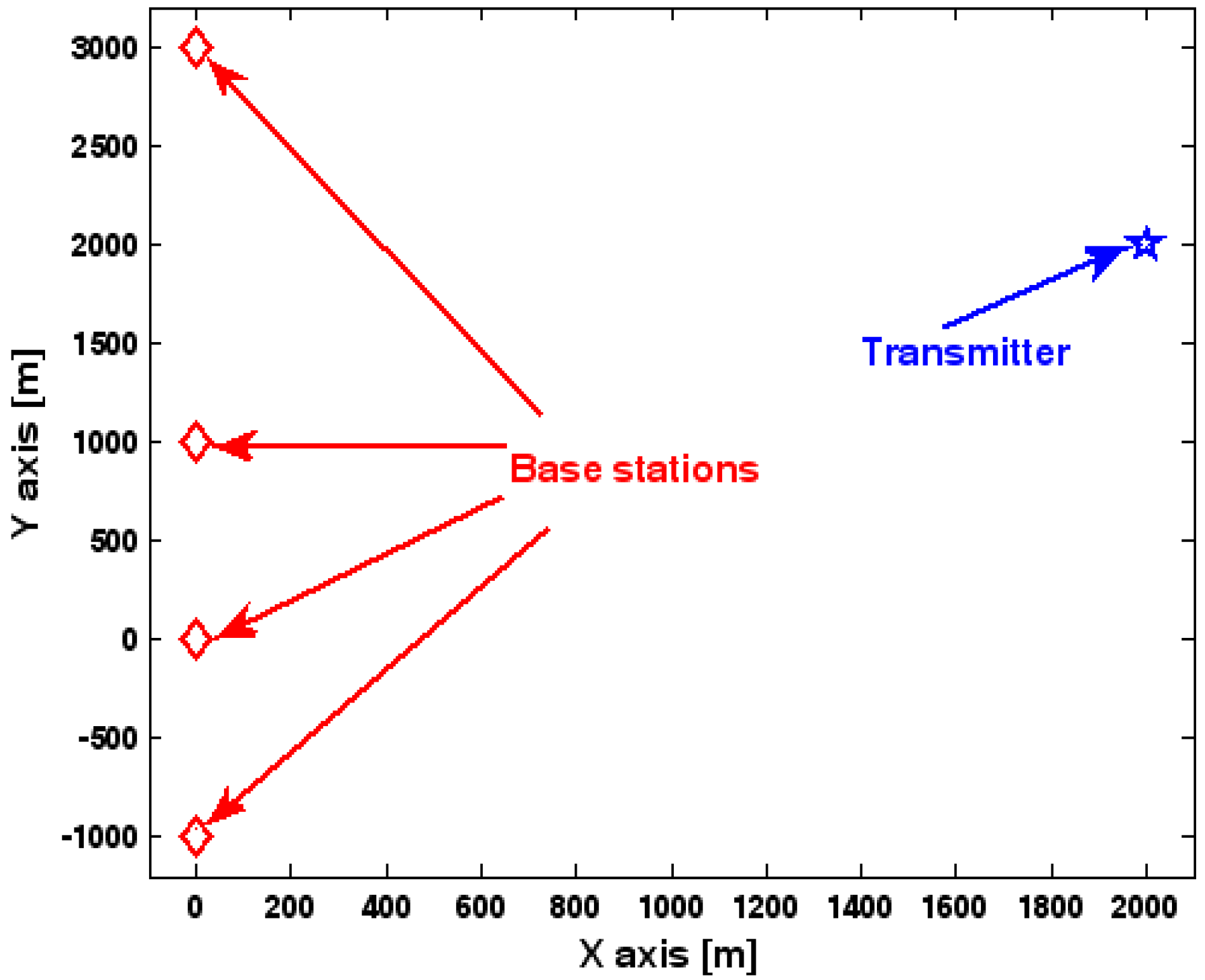
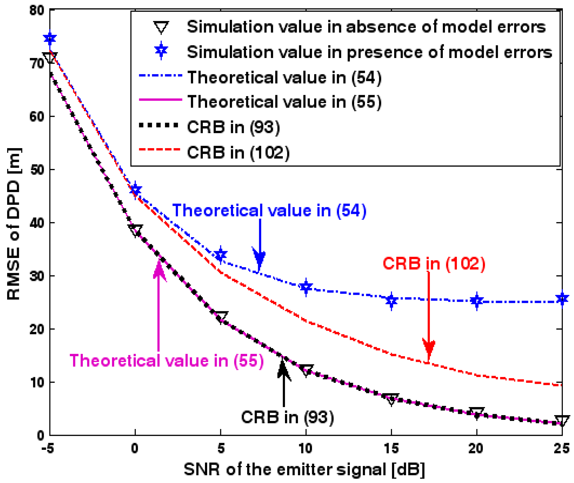
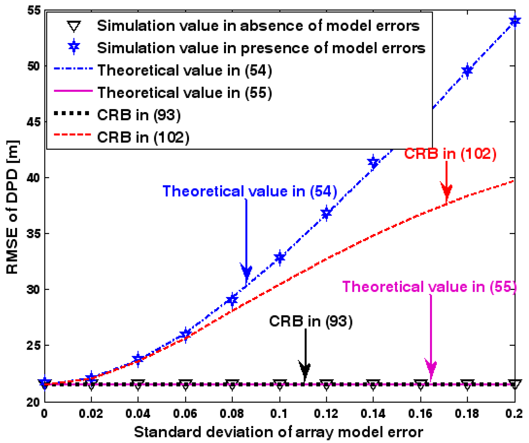
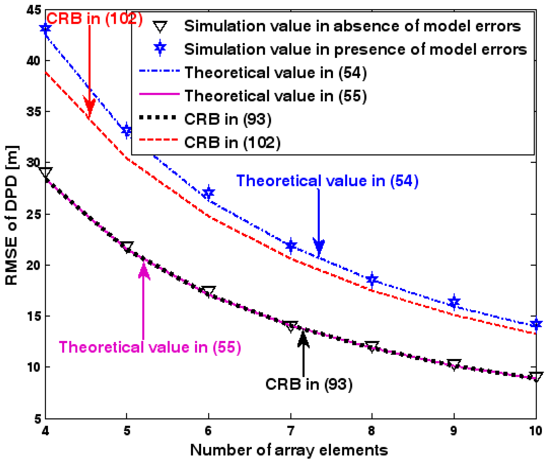
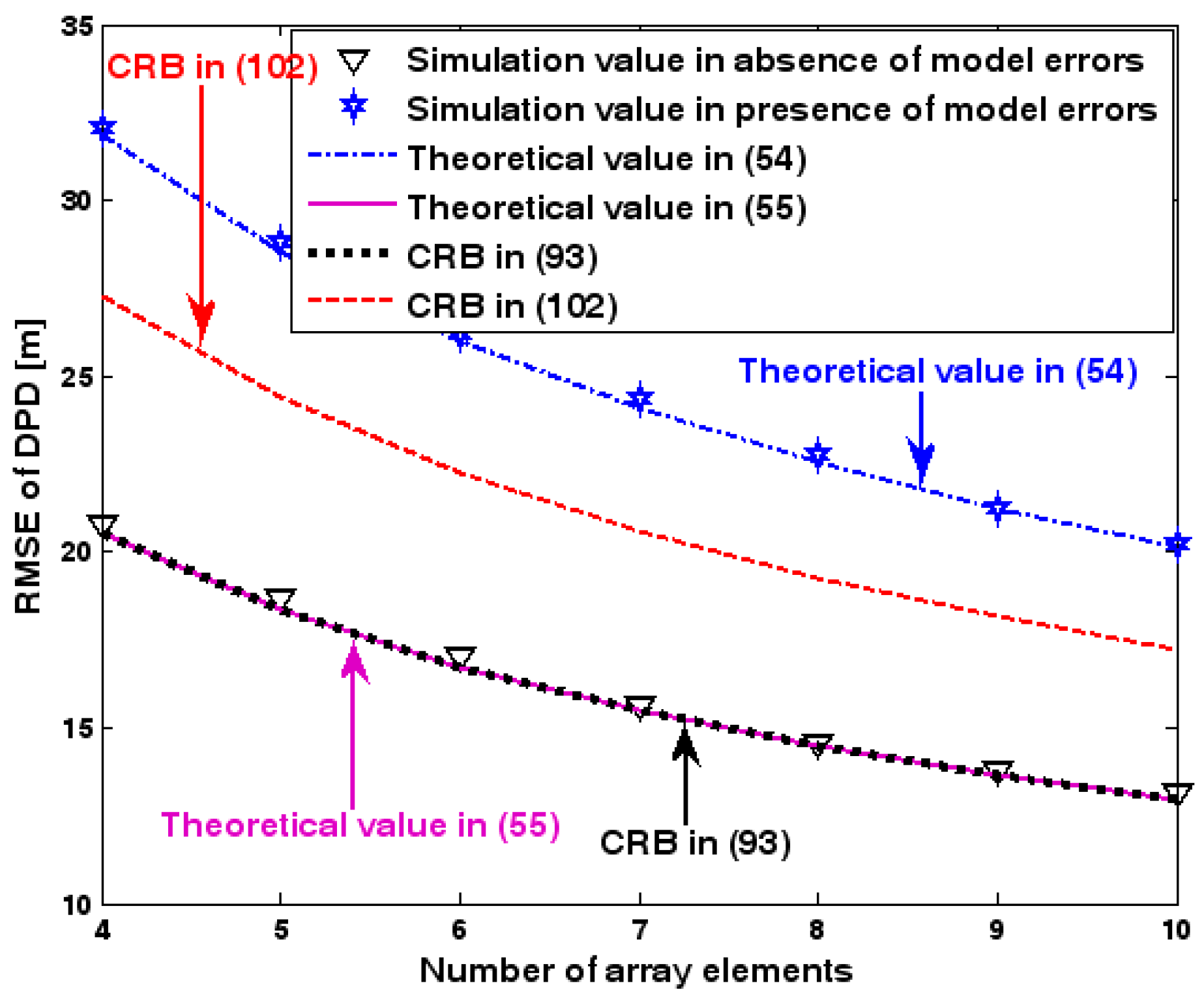
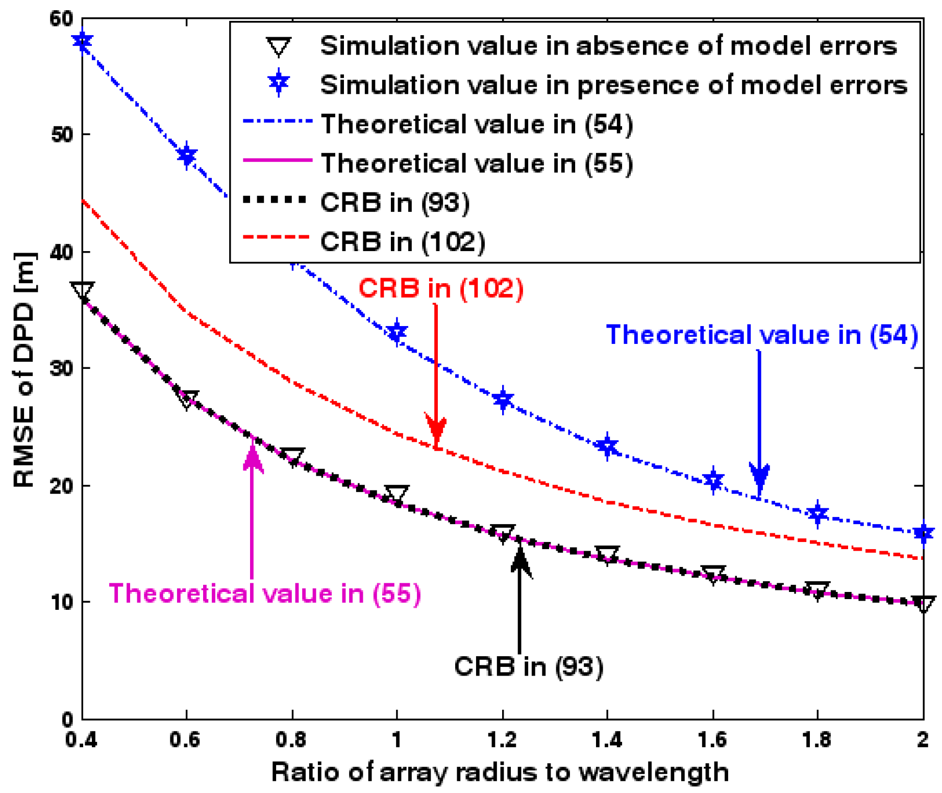
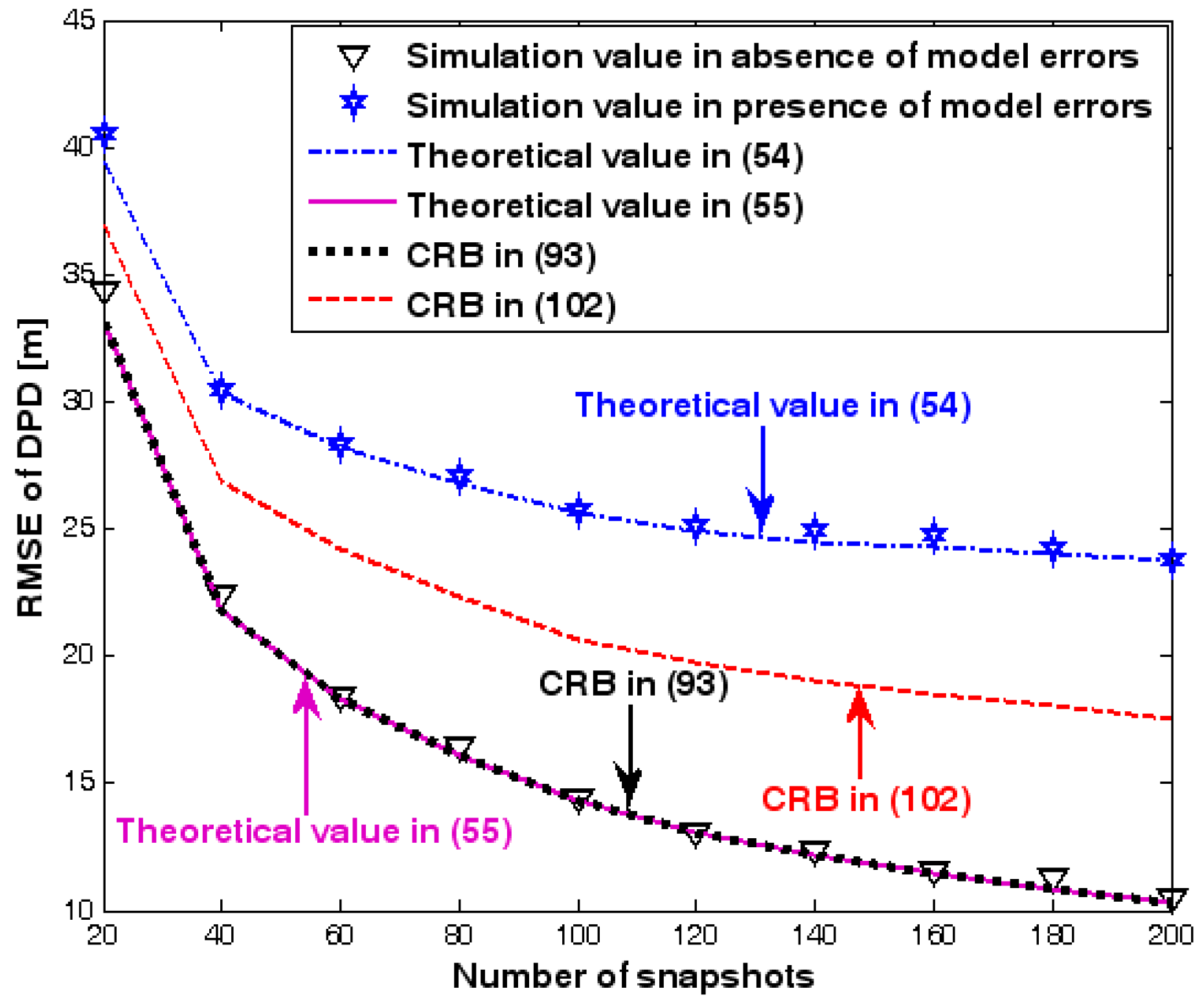
The location geometry of the first set of experiments is shown in Figure 1, where both base stations and transmitter lie on a plane. We consider four base stations with coordinates [0, 1000] m, [0,0] m, [0,1000] m, and [0, 3000] m, while the emitter position is fixed at [2000, 2000] m. The transmitted waveforms are realizations of a normal Gaussian random process, and are unknown to the receivers. Each base station is equipped with a uniform linear array. The channel attenuation magnitude is fixed at 1, and the channel phase is selected at random from a uniform distribution over [−π, π). In addition, unless stated otherwise, we use the settings (1) samples; (2) SNR of 5 dB; (3) sensors; (4) ; and (5) sensor elements are separated by a half wavelength. Figure 2, Figure 3, Figure 4, Figure 5 and Figure 6 display the RMSEs of the DPD method, as functions of the SNR of the emitter signal, the standard deviation of array model error , the number of array elements , the ratio of the intersensor spacing to wavelength, and the number of snapshots .
Figure 2, Figure 3, Figure 4, Figure 5 and Figure 6 reveal that the theoretical RMSE provided by (54) is in close agreement with the simulation result in the presence of array model errors. Consequently, the validity of the theoretical study in Section 6 is confirmed. Furthermore, when array model errors are absent, the empirical RMSE is very close to the CRB given by (92) and the theoretical RMSE in (55), which implies the asymptotical efficiency of the DPD method presented in [29], provided that the array is accurately calibrated. It is also seen that, as expected, the presence of array model errors leads to considerable deteriorations in location accuracy. Furthermore, Figure 2 and Figure 6 show that the RMSE of the DPD method remains approximately constant no matter how much the SNR and sample number increase. The reason for this is that when the SNR or the sample number is large enough, the effects of sensor noise can be neglected and the localization errors are therefore primarily caused by array model errors, whose affects cannot be effectively eliminated in this DPD method yet. Additionally, we find that the RMSE performance in the presence of array uncertainties is significantly greater than the CRB provided by (102), especially when the standard deviation increases (see Figure 3). Consequently, a new DPD method that accounts for array model errors is needed to improve the location accuracy.
9.1.2. The Second Set of Experiments
In the second set of experiments, the source location is estimated in 3-D space and we assume that the array error is caused by sensor gain and phase uncertainties, which corresponds to case 2 in Section 4 in [44]. The second-order moments of can then be expressed as
where and are the sensor gain and phase perturbation standard deviation, respectively. Moreover, we assume hereafter, and thus if is changed, alters accordingly.
Figure 7 illustrates the geometry for the source location in the second set of experiments. Obviously, it depicts a 3-D localization scenario. The source is positioned at [1000, 500, 1500] m, and the coordinates of three base stations are set to [0, 2000, 0] m, [0, 0, 0] m, and [0, −2000, 0] m. Each base station is equipped with a uniform circular array. The envelope of the transmitted signal and array model errors are generated in exactly the same manner as previously. Additionally, unless stated otherwise, we adopt the settings (1) samples; (2) SNR of 5 dB; (3) sensors; (4) ; and (5) an array radius equal to the wavelength. Figure 8, Figure 9, Figure 10, Figure 11 and Figure 12 show the RMSEs of the DPD method by varying the SNR of the emitter signal, standard deviation of sensor gain perturbation , the number of array elements , the ratio of array radius to wavelength, and the number of snapshots .
The results presented in Figure 8, Figure 9, Figure 10, Figure 11 and Figure 12 coincide with the results presented Figure 2, Figure 3, Figure 4, Figure 5 and Figure 6 although the dimensionality of the localization scenario and the model of the array error differ from each other. Owing to limited space, we do not present the results again. We simply highlight that the good agreement between the empirical and theoretical RMSE once again demonstrates the effectiveness of the theoretical development in Section 6.
9.2. Discussion on Success Probability of Direct Localization
This subsection focuses on the SP of the DPD method. Two sets of experiments are carried out to validate the obtained probability formulas, and the simulation parameters are the same as those in Section 9.1.
9.2.1. The First Set of Experiments
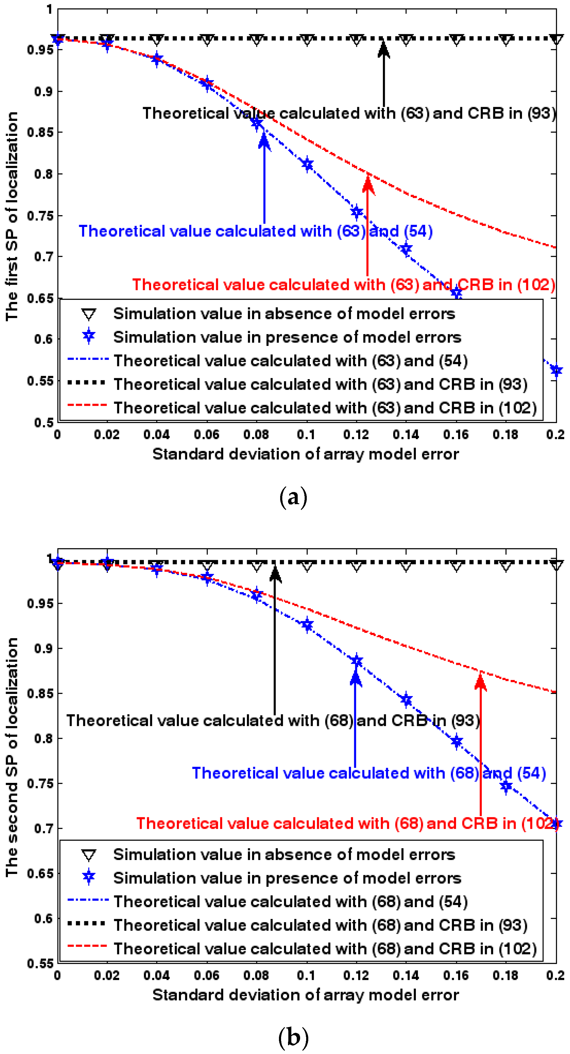
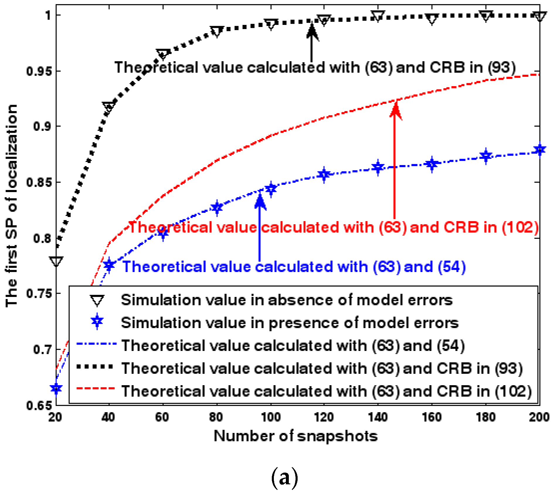
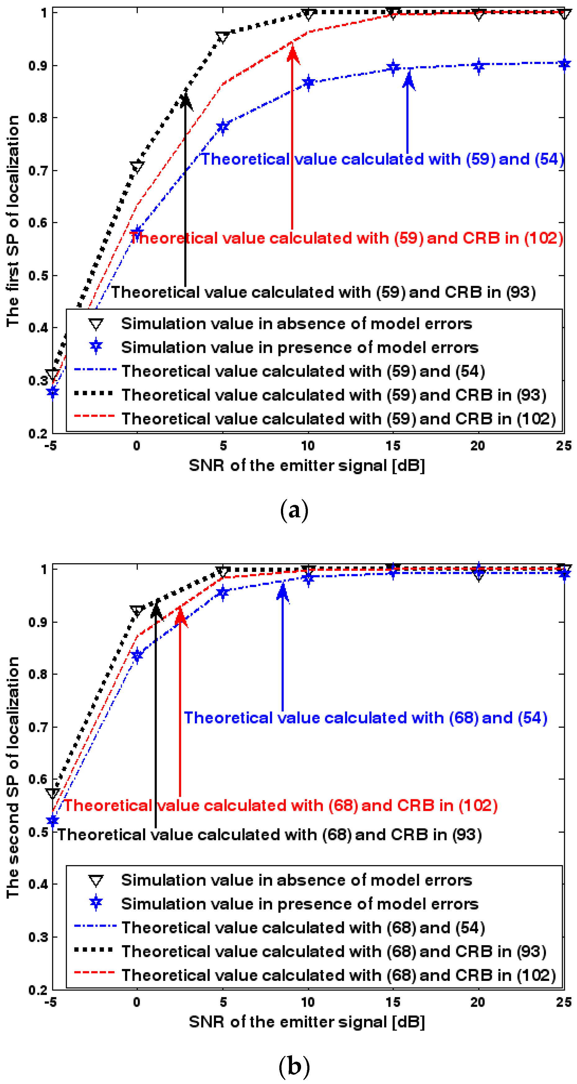
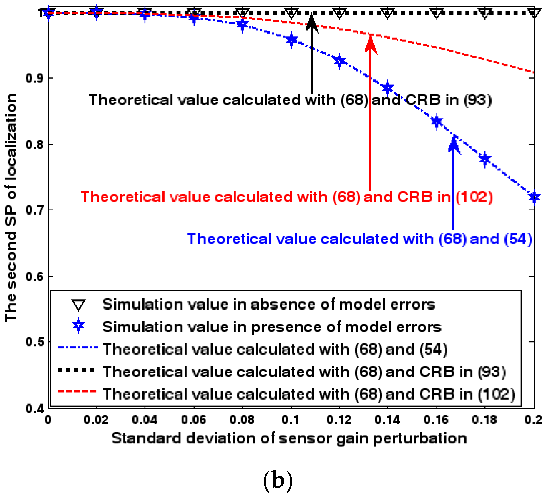
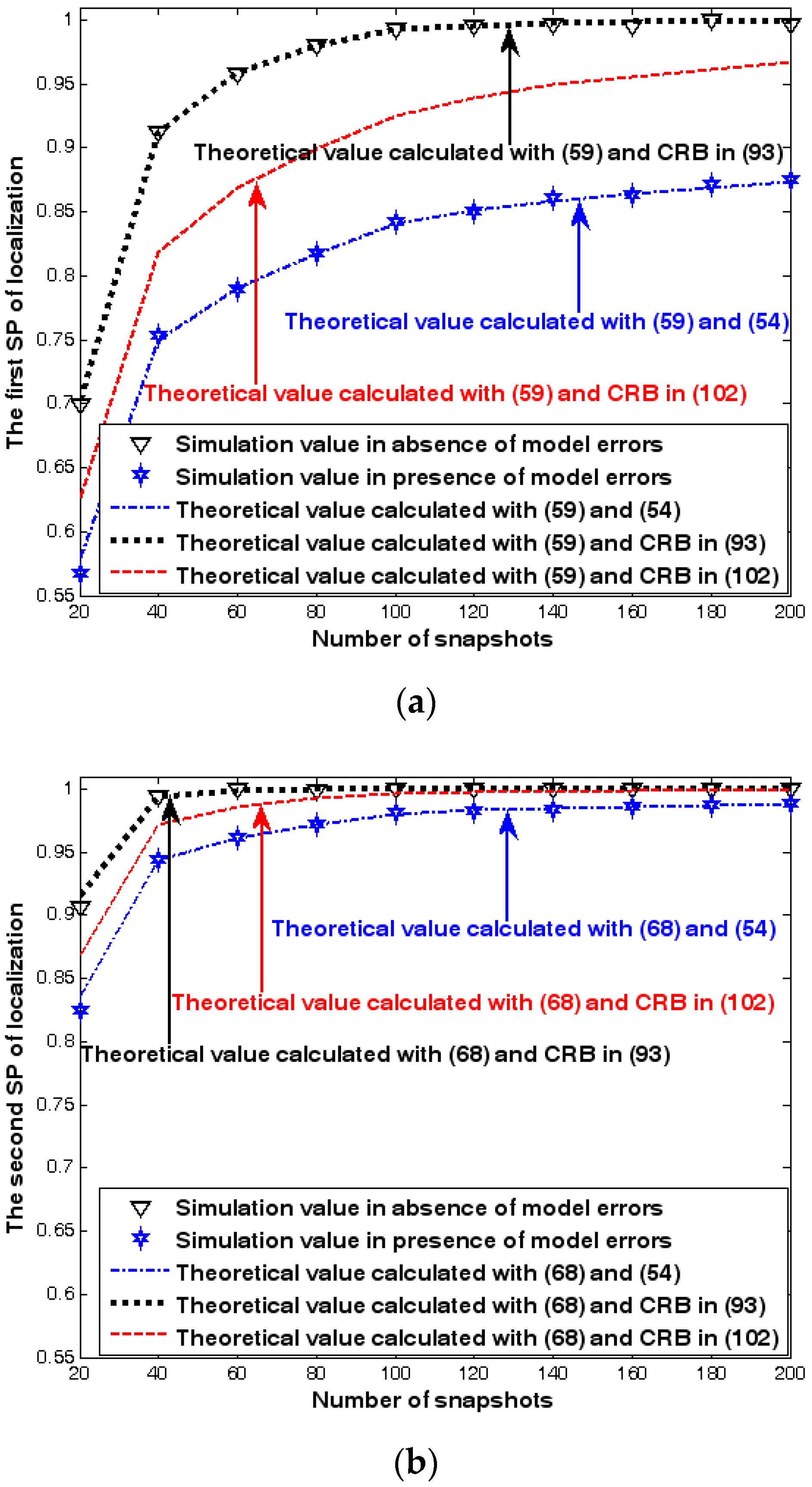
Both the localization scenario and the array error model for the first set of experiments are the same as those in Section 9.1.1. Moreover, the parameters and , which are used to specify the first SP, are set to the same value of 40, and the parameter , which is related to the second SP, is also selected as 40. Because the localization scenario is on a 2-D plane, the theoretical value of the first SP can be obtained with (63). In Figure 13, Figure 14 and Figure 15, we plot the two kinds of SP of the DPD method against the SNR of the emitter signal, standard deviation of the array model error , and number of snapshots .
Figure 13, Figure 14 and Figure 15 reveal that there is a close match between the analytical results and the simulation results and hence the validity of (63) and (68) can be supported. Furthermore, the simulated values in the absence of array model errors approach the lower bound calculated with the CRB in (93), which further indicates that the DPD estimator can achieve the CRB accuracy as long as the array is perfectly calibrated. However, when array model errors exist, the empirical values deviate significantly from the lower bound. Moreover, the difference increases with the standard deviation of array model error (see Figure 14). We thus need to develop a new DPD estimator with improved robustness against array model errors. Furthermore, it is seen that the first SP is always smaller than the second SP, which is consistent with the analysis in Remark 11.
9.2.2. The Second Set of Experiments
Both the localization scenario and the array error model for the second set of experiments are the same as those in Section 9.1.2. Because the situation is a 3-D localization scenario, the theoretical value of the first SP must be calculated with numerical integration methods. Herein, the Richardson extrapolation algorithm is exploited. Figure 16, Figure 17 and Figure 18 depict the two kinds of SP of the DPD method as functions of the SNR of the emitter signal, standard deviation of sensor gain perturbation , and number of snapshots .
9.3. Discussion on Radius of CEP
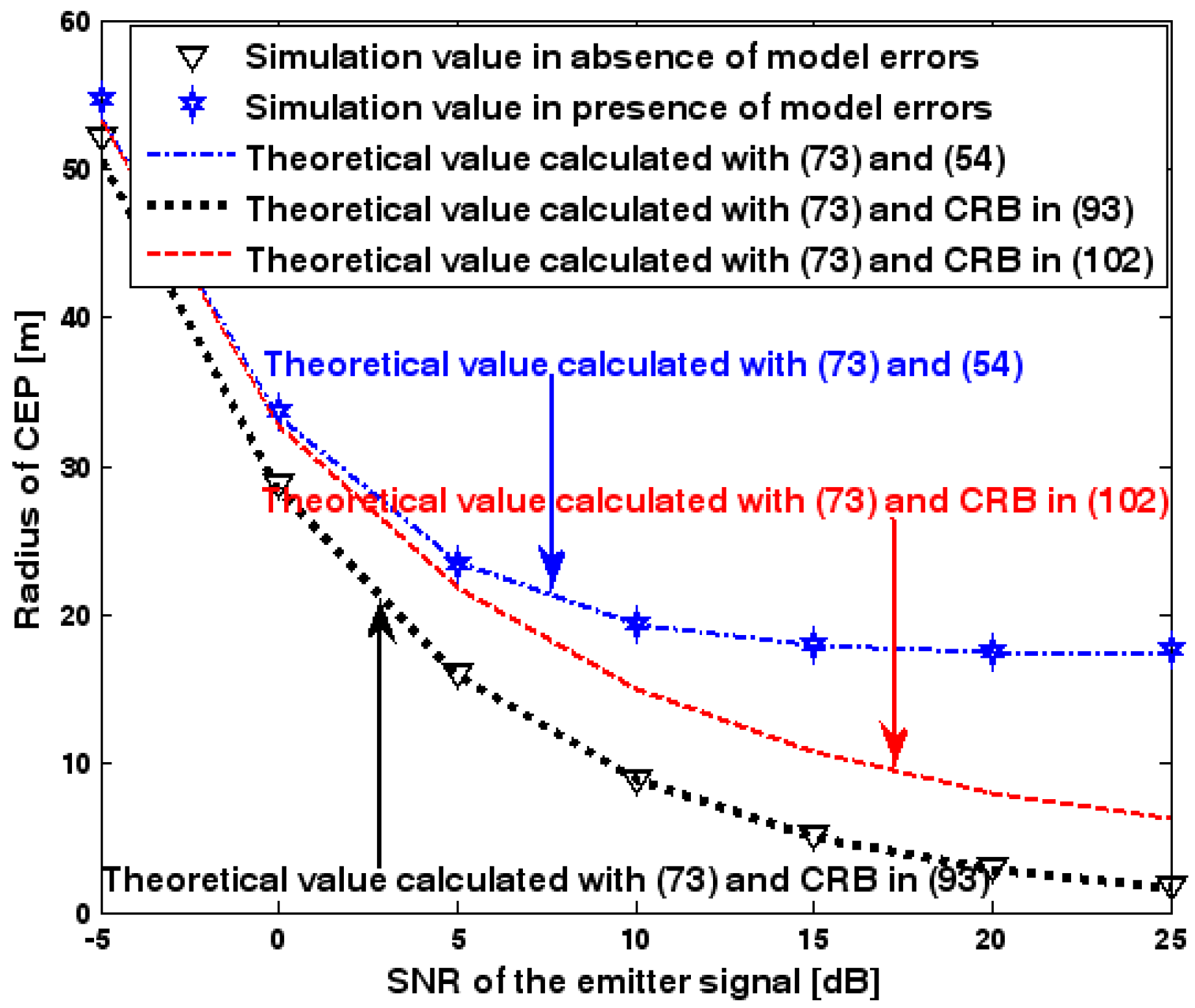
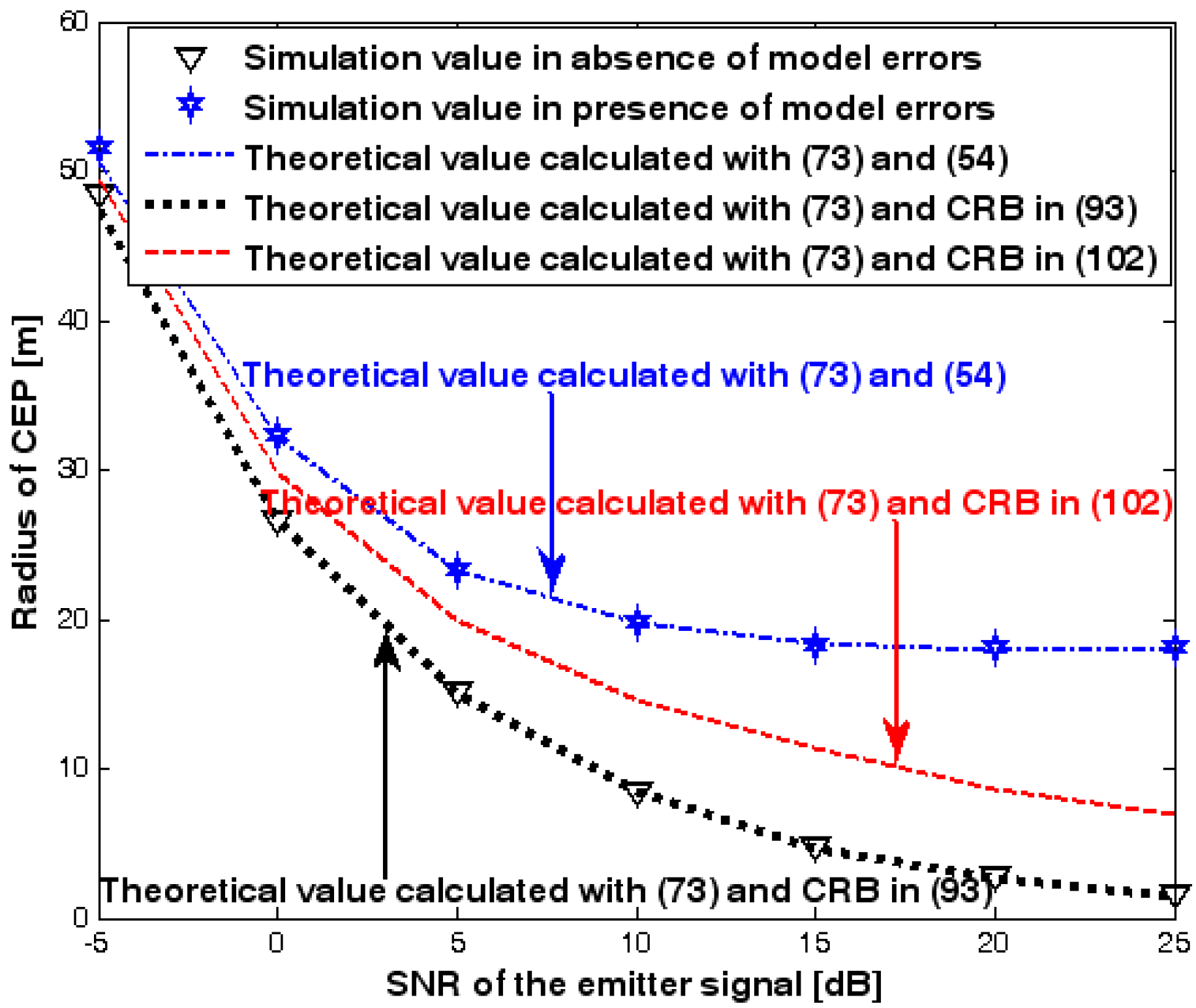
This subsection discusses the radius of CEP of the DPD method. Two simulation experiments are conducted to illustrate the validity of (73), which is used to estimate the radius of CEP. The first and second simulation settings are the same as those in Figure 2 and Figure 8, respectively. In the following two figures, the radius of CEP of the DPD method in the two experiments is plotted as a function of the SNR of the emitter signal.
Figure 19 and Figure 20 show that the simulation results agree well with the analytical results calculated with (73) and therefore the validity of (73) is corroborated. Moreover, we observe that the increase in the radius of CEP due to the array model errors is significant, especially when the SNR of the emitter signal is sufficiently high. Furthermore, when array model errors exist, the radius of CEP remains approximately constant no matter how much the SNR increases. Therefore, a robust DPD method that restrains the uncertainties in an array manifold is required.
10. Conclusions
In this paper, the statistical performance of the DPD estimator presented in [29] is analytically studied when array model errors are present as well as signal waveforms are not available. The theoretical analysis begins with a matrix eigen-perturbation result, which can express the perturbation of eigenvalues as a function of the disturbance added to the Hermitian matrix. Then, the first-order asymptotic expression of the localization errors is given, from which the analytical expression for the MSE of the DPD estimator is obtained. Besides, the closed-form expressions for the calculation of the probabilities of a successful localization are also deduced, which can offer another theoretical perspective on the study of the localization accuracy. Additionally, the obtained probability formula can be used to provide a new criterion to estimate the radius of CEP. Finally, the CRB expressions for the position estimation are derived for two cases: (a) array model errors do not exist, and (b) array model errors are present and are drawn from Gaussian distribution. Several simulation experiments are performed to confirm the usefulness of the obtained results. The experimental results show that the uncertainties in the model of the array manifold can seriously deteriorate the source location accuracy of the DPD method. Therefore, our future work is to present a new DPD method that is expected to be more robust against the array model errors.
Acknowledgments
The author would like to thank all the anonymous reviewers for their valuable comments and suggestions which vastly improved the content and presentation of this paper. The author also acknowledges support from National Natural Science Foundation of China (Grant No. 61201381 and No. 61401513), China Postdoctoral Science Foundation (Grant No. 2016M592989), the Self-Topic Foundation of Information Engineering University (Grant No. 2016600701), and the Outstanding Youth Foundation of Information Engineering University (Grant No. 2016603201).
Author Contributions
Ding Wang wrote the manuscript and Hongyi Yu helped with the writing, data analysis, and publication process. Zhidong Wu and Cheng Wang was in charge of the experiment and its results. All authors have contributed to the scientific discussion.
Conflicts of Interest
The authors declare no conflict of interest.
Appendix A—Detailed Derivation of Matrices in (30)
It follows from the first equality in (9) and the first equality in (12) that
where
Appendix B—Proof of (34) and (35)
Applying Proposition 1 and (31) leads to
where and consist of all first- and second-order error terms, respectively. It then follows that
Inserting the second equality in (32) into the first equality in (A6) leads to
Substituting the second and third equalities in (32) into the second equality in (A6) leads to
Combining (A7) and (A8) completes the proof.
Appendix C—Proof of (36) to (38)
From the second equality in (29), it follows for any vectors and that
According to the last equality in (17), it can be readily checked that
where is given in the first equality in (38). With (21), we have
where is given in the second equality in (38). In addition, it can be easily verified that
where is given in the third equality in (38). Combining (A9) to (A12) yields
It follows easily from (A13) that
which, combined with (23) and (25), gives
Combining (A14), (A15), and the first equality in (35) completes the proof.
Appendix D—Proof of (39) to (44)
For any vectors and and matrix , it is straightforward to obtain that
Inserting (A13) into (A16) produces
where are given in (41).
For any vectors and and matrix , it can be readily checked that
Putting (A13) into (A18) gives
where are given in (42).
For any vectors and and matrix , it is straightforward to deduce that
The substitution of (A13) into (A20) leads to
where are given in (43).
For any vectors and , it can be easily verified from the third equality in (29) that
According to the last equality in (17), we get
where is given in the first equality in (44). It follows from (21) that
where is given in the second equality in (44). In addition, it can be easily verified that
where is given in the third equality in (44). Combining (A22) to (A25) gives
With (A17) we have
which, together with (23) and (25), gives
Applying (A19), it can be shown that
According to (A21), we have
Additionally, it follows from (A26) that
which, together with (23) and (25), gives
Combining (A27) to (A32) and the second equality in (35) completes the proof.
Appendix E—Proof of Proposition 2
First introduce the event . The joint probability can then be expressed as
It is obvious that
Additionally, random variable can be decomposed with classical minimum-MSE theory into
where is drawn from a zero-mean Gaussian distribution, independent of , with variance
According to (A35), it can be verified that
where and . Applying the incomplete moment theory presented in [28], we get
Inserting (A39) back into (A37) yields
Furthermore, substituting (A39) and (A40) into (A38) leads to
which together with (A41) gives
Applying (A41) and (A43) produces
Combining (A33), (A34), and (A44) completes the proof.
Appendix F—Proof of (62)
Making use of simple properties of probability, it can be readily verified that
Likewise, we have
Inserting (A46) and (A47) back into (A45) yields (62).
Appendix G—Detailed Derivation of Matrices in (92)
Performing algebraic manipulation, and using (80), we have
Firstly, inserting (A48), (A49), and (A51) into the first equality in (92) yields
Secondly, substituting (A49), (A51), (A52), and (A53) into the second equality in (92) gives
where
Finally, putting (A49), (A50), and (A53) into the third equality in (92) leads to
Appendix H—Proof of (96)
We start by introducing a real array model error vector with probability density function given by
When the deterministic and stochastic parameters coexist, the Fisher information matrix (FIM) for vector is given by [68,69],
where is the ML function of the compound data vector . Combining (A59) and the results in [66,67], the FIM for vector can be expressed as
where is an indicator function such that if both and correspond to the element in , and otherwise. It follows from (A60) that
which completes the proof.
Appendix I—Detailed Derivation of Matrices in (101)
Note that matrices , , , , , and are given in (A48) to (A53). Therefore, to calculate the matrices in (101), we only need to derive the expressions for matrices , , , and . It follows from (99) that
References
- Schmidt, R.O. Multiple emitter location and signal parameter estimation. IEEE Trans. Antennas Propag. 1986, 34, 267–280. [Google Scholar] [CrossRef]
- Stoica, P.; Nehorai, A. MUSIC, maximum likelihood, and Cramér-Rao bound. IEEE Trans. Acoust. Speech Signal Process. 1989, 37, 720–741. [Google Scholar] [CrossRef]
- Viberg, M.; Ottersten, B. Sensor array processing based on subspace fitting. IEEE Trans. Signal Process. 1991, 39, 1110–1121. [Google Scholar] [CrossRef]
- Liao, B.; Chan, S.C.; Huang, L.; Guo, C. Iterative methods for subspace and DOA estimation in nonuniform noise. IEEE Trans. Signal Process. 2016, 64, 3008–3020. [Google Scholar] [CrossRef]
- Sun, F.; Gao, B.; Chen, L.; Lan, P. A low-complexity ESPRIT-based DOA estimation method for co-prime linear arrays. Sensors 2016, 16, 1367. [Google Scholar] [CrossRef] [PubMed]
- Nardone, S.C.; Graham, M.L. A closed-form solution to bearings-only target motion analysis. IEEE J. Ocean. Eng. 1997, 22, 168–178. [Google Scholar] [CrossRef]
- Kutluyil, D. Bearings-only target localization using total least squares. Signal Process. 2005, 85, 1695–1710. [Google Scholar]
- Lin, Z.; Han, T.; Zheng, R.; Fu, M. Distributed localization for 2-D sensor networks with bearing-only measurements under switching topologies. IEEE Trans. Signal Process. 2016, 64, 6345–6359. [Google Scholar] [CrossRef]
- Yang, K.; An, J.; Bu, X.; Sun, G. Constrained total least-squares location algorithm using time-difference-of-arrival measurements. IEEE Trans. Veh. Technol. 2010, 59, 1558–1562. [Google Scholar] [CrossRef]
- Jiang, W.; Xu, C.; Pei, L.; Yu, W. Multidimensional Scaling-Based TDOA Localization Scheme Using an Auxiliary Line. IEEE Signal Process. Lett. 2016, 23, 546–550. [Google Scholar] [CrossRef]
- Ma, Z.H.; Ho, K.C. TOA localization in the presence of random sensor position errors. In Proceedings of the IEEE International Conference on Acoustics, Speech and Signal Processing, Prague, Czech, 22–27 May 2011; pp. 2468–2471. [Google Scholar]
- Shen, H.; Ding, Z.; Dasgupta, S.; Zhao, C. Multiple source localization in wireless sensor networks based on time of arrival measurement. IEEE Trans. Signal Process. 2014, 62, 1938–1949. [Google Scholar] [CrossRef]
- Yu, H.G.; Huang, G.M.; Gao, J.; Liu, B. An efficient constrained weighted least squares algorithm for moving source location using TDOA and FDOA measurements. IEEE Trans. Wirel. Commun. 2012, 11, 44–47. [Google Scholar] [CrossRef]
- Wang, G.; Li, Y.; Ansari, N. A semidefinite relaxation method for source localization Using TDOA and FDOA Measurements. IEEE Trans. Veh. Technol. 2013, 62, 853–862. [Google Scholar] [CrossRef]
- Mason, J. Algebraic two-satellite TOA/FOA position solution on an ellipsoidal earth. IEEE Trans. Aerosp. Electron. Syst. 2004, 40, 1087–1092. [Google Scholar] [CrossRef]
- Cheung, K.W.; So, H.C.; Ma, W.K.; Chan, Y.T. Received signal strength based mobile positioning via constrained weighted least squares. In Proceedings of the IEEE International Conference on Acoustic, Speech and Signal Processing, Hong Kong, China, 6–8 April 2003; pp. 137–140. [Google Scholar]
- Ho, K.C.; Sun, M. An accurate algebraic closed-form solution for energy-based source localization. IEEE Trans. Audio Speech Lang. Process. 2007, 15, 2542–2550. [Google Scholar] [CrossRef]
- Wax, M.; Kailath, T. Decentralized processing in sensor arrays. IEEE Trans. Signal Process. 1985, 33, 1123–1129. [Google Scholar] [CrossRef]
- Stoica, P. On reparametrization of loss functions used in estimation and the invariance principle. Signal Process. 1989, 17, 383–387. [Google Scholar] [CrossRef]
- Amar, A.; Weiss, A.J. Localization of narrowband radio emitters based on Doppler frequency shifts. IEEE Trans. Signal Process. 2008, 56, 5500–5508. [Google Scholar] [CrossRef]
- Wang, D.; Wu, Y. Statistical performance analysis of direct position determination method based on doppler shifts in presence of model errors. Multidimens. Syst. Signal Process. 2017, 28, 149–182. [Google Scholar] [CrossRef]
- Tzoreff, E.; Weiss, A.J. Expectation-maximization algorithm for direct position determination. Signal Process. 2017, 97, 32–39. [Google Scholar] [CrossRef]
- Vankayalapati, N.; Kay, S.; Ding, Q. TDOA based direct positioning maximum likelihood estimator and the Cramer-Rao bound. IEEE Trans. Aerosp. Electron. Syst. 2014, 50, 1616–1634. [Google Scholar] [CrossRef]
- Xia, W.; Liu, W.; Zhu, L.F. Distributed adaptive direct position determination based on diffusion framework. J. Syst. Eng. Electron. 2016, 27, 28–38. [Google Scholar]
- Weiss, A.J. Direct geolocation of wideband emitters based on delay and Doppler. IEEE Trans. Signal Process. 2011, 59, 2513–5520. [Google Scholar] [CrossRef]
- Pourhomayoun, M.; Fowler, M.L. Distributed computation for direct position determination emitter location. IEEE Trans. Aerosp. Electron. Syst. 2014, 50, 2878–2889. [Google Scholar] [CrossRef]
- Bar-Shalom, O.; Weiss, A.J. Emitter geolocation using single moving receiver. Signal Process. 2014, 94, 70–83. [Google Scholar] [CrossRef]
- Li, J.Z.; Yang, L.; Guo, F.C.; Jiang, W.L. Coherent summation of multiple short-time signals for direct positioning of a wideband source based on delay and Doppler. Digit. Signal Process. 2016, 48, 58–70. [Google Scholar] [CrossRef]
- Weiss, A.J. Direct position determination of narrowband radio frequency transmitters. IEEE Signal Process. Lett. 2004, 11, 513–516. [Google Scholar] [CrossRef]
- Weiss, A.J.; Amar, A. Direct position determination of multiple radio signals. EURASIP J. Appl. Signal Process. 2005, 2005, 37–49. [Google Scholar] [CrossRef]
- Amar, A.; Weiss, A.J. A decoupled algorithm for geolocation of multiple emitters. Signal Process. 2007, 87, 2348–2359. [Google Scholar] [CrossRef]
- Tirer, T.; Weiss, A.J. High resolution direct position determination of radio frequency sources. IEEE Signal Process. Lett. 2016, 23, 192–196. [Google Scholar] [CrossRef]
- Tzafri, L.; Weiss, A.J. High-resolution direct position determination using MVDR. IEEE Trans. Wirel. Commun. 2016, 15, 6449–6461. [Google Scholar] [CrossRef]
- Amar, A.; Weiss, A.J. Direct position determination in the presence of model errors—known waveforms. Digit. Signal Process. 2006, 16, 52–83. [Google Scholar] [CrossRef]
- Demissie, B. Direct localization and detection of multiple sources in multi-path environments. In Proceedings of the IEEE International Conference on Information Fusion, Chicago, IL, USA, 5–8 July 2011; pp. 1–8. [Google Scholar]
- Papakonstantinou, K.; Slock, D. Direct location estimation for MIMO systems in multipath environments. In Proceedings of the IEEE International Conference on Global Telecommunications, New Orleans, LA, USA, 30 November–4 December 2008; pp. 1–5. [Google Scholar]
- Bar-Shalom, O.; Weiss, A.J. Efficient direct position determination of orthogonal frequency division multiplexing signals. IET Radar Sonar Navig. 2009, 3, 101–111. [Google Scholar] [CrossRef]
- Reuven, A.M.; Weiss, A.J. Direct position determination of cyclostationary signals. Signal Process. 2009, 89, 2448–2464. [Google Scholar] [CrossRef]
- Oispuu, M.; Nickel, U. Direct detection and position determination of multiple sources with intermittent emission. Signal Process. 2010, 90, 3056–3064. [Google Scholar] [CrossRef]
- Shen, J.; Shen, J.; Chen, X.F.; Huang, X.Y.; Susilo, W. An efficient public auditing protocol with novel dynamic structure for cloud data. IEEE Trans. Inf. Forensics Secur. 2017, PP, 1. [Google Scholar] [CrossRef]
- Fu, Z.J.; Ren, K.; Shu, J.G.; Sun, X.M.; Huang, F.X. Enabling personalized search over encrypted outsourced data with efficiency improvement. IEEE Trans. Parallel Distrib. Syst. 2016, 27, 2546–2559. [Google Scholar] [CrossRef]
- Sun, Y.J.; Gu, F.H. Compressive sensing of piezoelectric sensor response signal for phased array structural health monitoring. Int. J. Sens. Netw. 2017, 23, 258–264. [Google Scholar] [CrossRef]
- Friedlander, B. A sensitivity analysis of the MUSIC algorithm. IEEE Trans. Acoust. Speech Signal Process. 1990, 38, 1740–1751. [Google Scholar] [CrossRef]
- Swindlehurst, A.; Kailath, T. A performance analysis of subspace-based methods in the presence of model errors, part I: The MUSIC algorithm. IEEE Trans. Signal Process. 1992, 40, 1758–1774. [Google Scholar] [CrossRef]
- Ferréol, A.; Larzabal, P.; Viberg, M. On the asymptotic performance analysis of subspace DOA estimation in the presence of modeling errors: Case of MUSIC. IEEE Trans. Signal Process. 2006, 54, 907–920. [Google Scholar] [CrossRef]
- Ferréol, A.; Larzabal, P.; Viberg, M. On the resolution probability of MUSIC in presence of modeling errors. IEEE Trans. Signal Process. 2008, 56, 1945–1953. [Google Scholar] [CrossRef]
- Ferréol, A.; Larzabal, P.; Viberg, M. Statistical analysis of the MUSIC algorithm in the presence of modeling errors, taking into account the resolution probability. IEEE Trans. Signal Process. 2010, 58, 4156–4166. [Google Scholar] [CrossRef]
- Inghelbrecht, V.; Verhaevert, J.; van Hecke, T.; Rogier, H. The influence of random element displacement on DOA estimates obtained with (Khatri-Rao-) root-MUSIC. Sensors 2014, 14, 21258–21280. [Google Scholar] [CrossRef] [PubMed]
- Huang, Z.T.; Liu, Z.M.; Liu, J.; Zhou, Y.Y. Performance analysis of MUSIC for non-circular signals in the presence of mutual coupling. IET Signal Process. 2010, 4, 703–711. [Google Scholar] [CrossRef]
- Khodja, M.; Belouchrani, A.; Abed-Meraim, K. Performance analysis for time-frequency MUSIC algorithm in presence of both additive noise and array calibration errors. EURASIP J. Adv. Signal Process. 2012, 2012, 94–104. [Google Scholar] [CrossRef]
- Hari, K.V.S.; Gummadavelli, U. Effect of spatial smoothing on the performance of subspace methods in the presence of array model errors. Automatica 1994, 30, 11–26. [Google Scholar] [CrossRef]
- Soon, V.C.; Huang, Y.F. An analysis of ESPRIT under random sensor uncertainties. IEEE Trans. Signal Process. 1992, 40, 2353–2358. [Google Scholar] [CrossRef]
- Swindlehurst, A.; Kailath, T. A performance analysis of subspace-based methods in the presence of model errors: Part II-Multidimensional algorithm. IEEE Trans. Signal Process. 1993, 41, 2882–2890. [Google Scholar] [CrossRef]
- Friedlander, B. Sensitivity analysis of the maximum likelihood direction-finding algorithm. IEEE Trans. Aerosp. Electron. Syst. 1990, 26, 708–717. [Google Scholar] [CrossRef]
- Ferréol, A.; Larzabal, P.; Viberg, M. Performance prediction of maximum-likelihood direction-of-arrival estimation in the presence of modeling errors. IEEE Trans. Signal Process. 2008, 56, 4785–4793. [Google Scholar] [CrossRef]
- Cao, X.; Xin, J.M.; Nishio, Y.; Zheng, N.N. Spatial signature estimation with an uncalibrated uniform linear array. Sensors 2015, 15, 13899–13915. [Google Scholar] [CrossRef] [PubMed]
- Wang, W.J.; Ren, S.W.; Ding, Y.T.; Wang, H.Y. An efficient algorithm for direction finding against unknown mutual coupling. Sensors 2014, 14, 20064–20077. [Google Scholar] [CrossRef] [PubMed]
- Weiss, A.J.; Friedlander, B. DOA and steering vector estimation using a partially calibrated array. IEEE Trans. Aerosp. Electron. Syst. 1996, 32, l047–l057. [Google Scholar] [CrossRef]
- Pesavento, M.; Gershman, A.B.; Wong, K.M. Direction finding in partly-calibrated sensor arrays composed of multiple subarrays. IEEE Trans. Signal Process. 2002, 55, 2103–2115. [Google Scholar] [CrossRef]
- Wang, B.; Wang, W.; Gu, Y.J.; Lei, S.J. Underdetermined DOA estimation of quasi-stationary signals using a partly-calibrated array. Sensors 2017, 17, 702. [Google Scholar] [CrossRef] [PubMed]
- Amar, A.; Weiss, A.J. Analysis of the direct position determination approach in the presence of model errors. In Proceedings of the IEEE Convention on Electrical and Electronics Engineers, Telaviv, Israel, 6–7 September 2004; pp. 408–411. [Google Scholar]
- Amar, A.; Weiss, A.J. Analysis of direct position determination approach in the presence of model errors. In Proceedings of the IEEE Workshop on Statistical Signal Processing, Novosibirsk, Russia, 17–20 July 2005; pp. 521–524. [Google Scholar]
- Rao, C.R. Linear Statistical Inference and Its Application, 2nd ed.; Wiley: New York, NY, USA, 2002. [Google Scholar]
- Imhof, J.P. Computing the distribution of quadratic forms in normal variables. Biometrika 1961, 48, 419–426. [Google Scholar] [CrossRef]
- Torrieri, D.J. Statistical theory of passive location systems. IEEE Trans. Aerosp. Electron. Syst. 1984, 20, 183–198. [Google Scholar] [CrossRef]
- Gu, H. Linearization method for finding Cramér-Rao bounds in signal processing. IEEE Trans. Signal Process. 2000, 48, 543–545. [Google Scholar]
- Stoica, P.; Larsson, E.G. Comments on “Linearization method for finding Cramér-Rao bounds in signal processing”. IEEE Trans. Signal Process. 2001, 49, 3168–3169. [Google Scholar] [CrossRef]
- Viberg, M.; Swindlehurst, A.L. A Bayesian approach to auto-calibration for parametric array signal processing. IEEE Trans. Signal Processing 1994, 42, 3495–3507. [Google Scholar] [CrossRef]
- Jansson, M.; Swindlehurst, A.L.; Ottersten, B. Weighted subspace fitting for general array error models. IEEE Trans. Signal Process. 1998, 46, 2484–2498. [Google Scholar] [CrossRef]
- Wang, D. Sensor array calibration in presence of mutual coupling and gain/phase errors by combining the spatial-domain and time-domain waveform information of the calibration sources. Circuits Syst. Signal Process. 2013, 32, 1257–1292. [Google Scholar] [CrossRef]
Figure 1.
Location geometry for simulation.

Figure 2.
Root-mean-square-error (RMSE) of direct position determination (DPD) versus signal-to-noise ratio (SNR) of the emitter signal.
Figure 2.
Root-mean-square-error (RMSE) of direct position determination (DPD) versus signal-to-noise ratio (SNR) of the emitter signal.

Figure 3.
RMSE of DPD versus standard deviation of array model error.

Figure 4.
RMSE of DPD versus number of array elements.

Figure 5.
RMSE of DPD versus ratio of intersensor spacing to wavelength.

Figure 6.
RMSE of DPD versus number of snapshots.

Figure 7.
Source location scenario for simulation.

Figure 8.
RMSE of DPD as a function of SNR of the emitter signal.

Figure 9.
RMSE of DPD as a function of standard deviation of sensor gain perturbation.
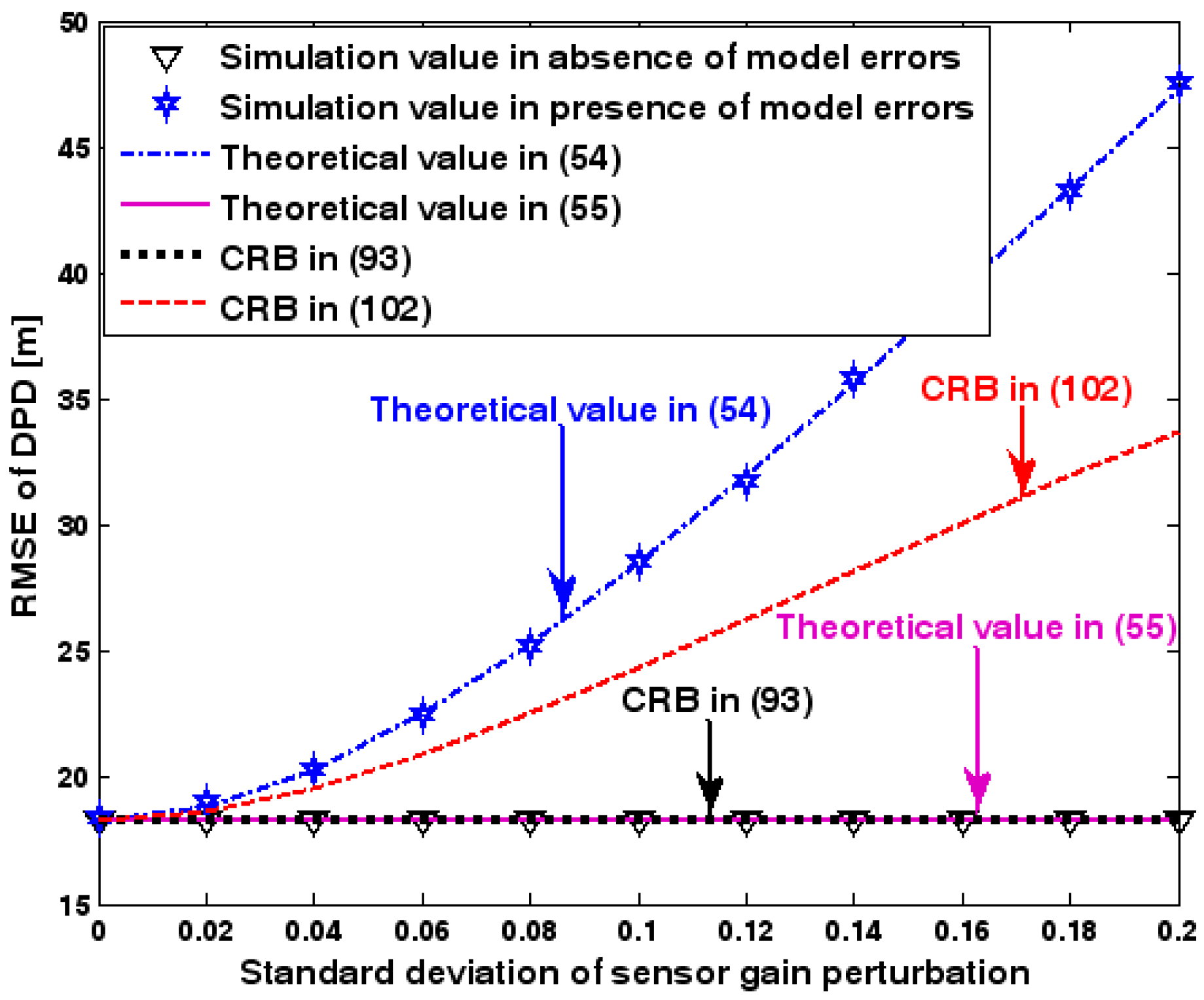
Figure 10.
RMSE of DPD as a function of number of array elements.

Figure 11.
RMSE of DPD as a function of ratio of array radius to wavelength.

Figure 12.
RMSE of DPD as a function of number of snapshots.

Figure 13.
Success probability (SP) of localization versus SNR of the emitter signal. (a) The first SP of localization versus SNR of the emitter signal. (b) The second SP of localization versus SNR of the emitter signal.
Figure 13.
Success probability (SP) of localization versus SNR of the emitter signal. (a) The first SP of localization versus SNR of the emitter signal. (b) The second SP of localization versus SNR of the emitter signal.
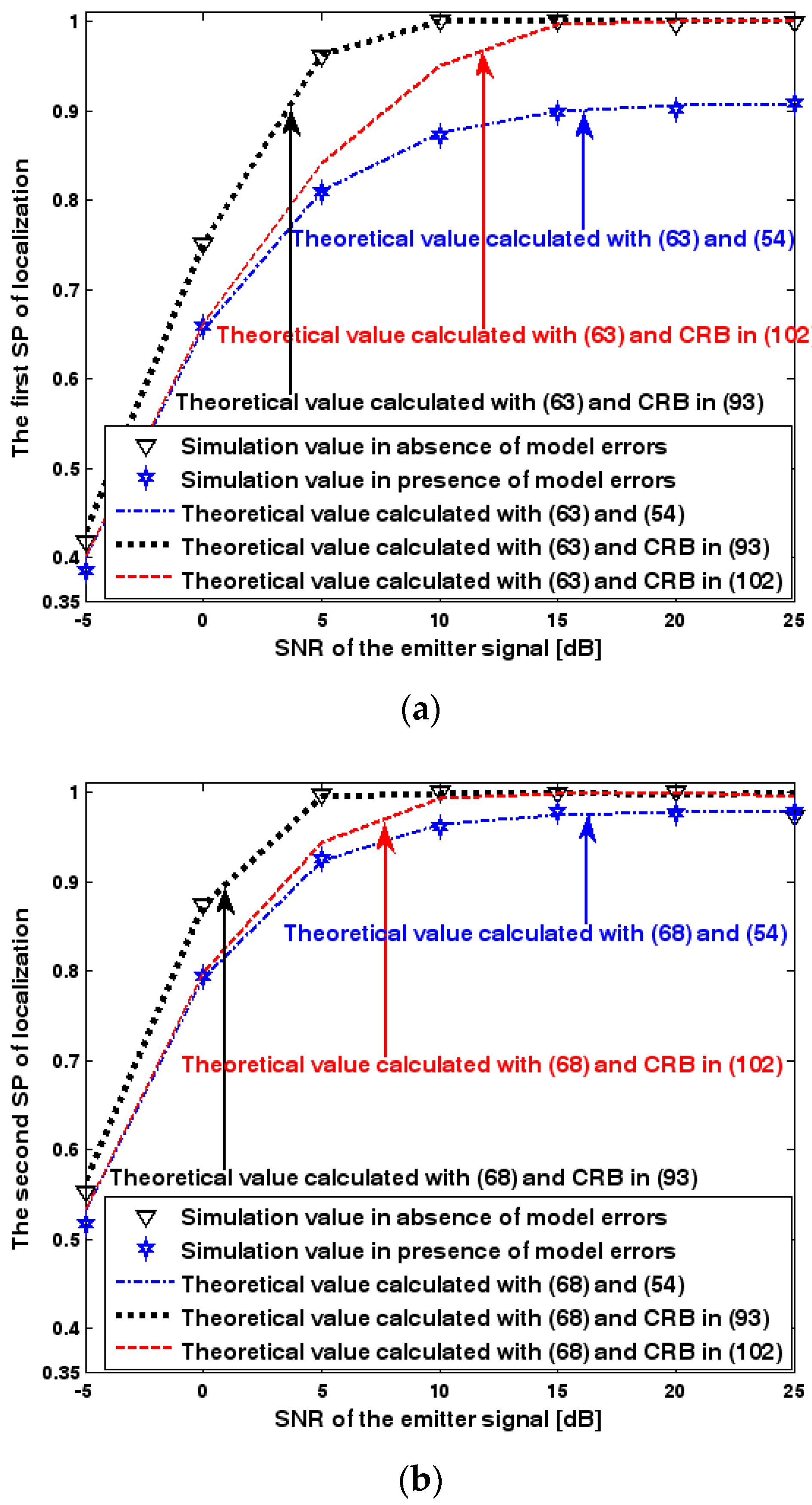
Figure 14.
SP of localization versus standard deviation of array model error. (a) The first SP of localization versus standard deviation of array model error. (b) The second SP of localization versus standard deviation of array model error.
Figure 14.
SP of localization versus standard deviation of array model error. (a) The first SP of localization versus standard deviation of array model error. (b) The second SP of localization versus standard deviation of array model error.

Figure 15.
SP of localization versus number of snapshots. (a) The first SP of localization versus number of snapshots. (b) The second SP of localization versus number of snapshots.
Figure 15.
SP of localization versus number of snapshots. (a) The first SP of localization versus number of snapshots. (b) The second SP of localization versus number of snapshots.

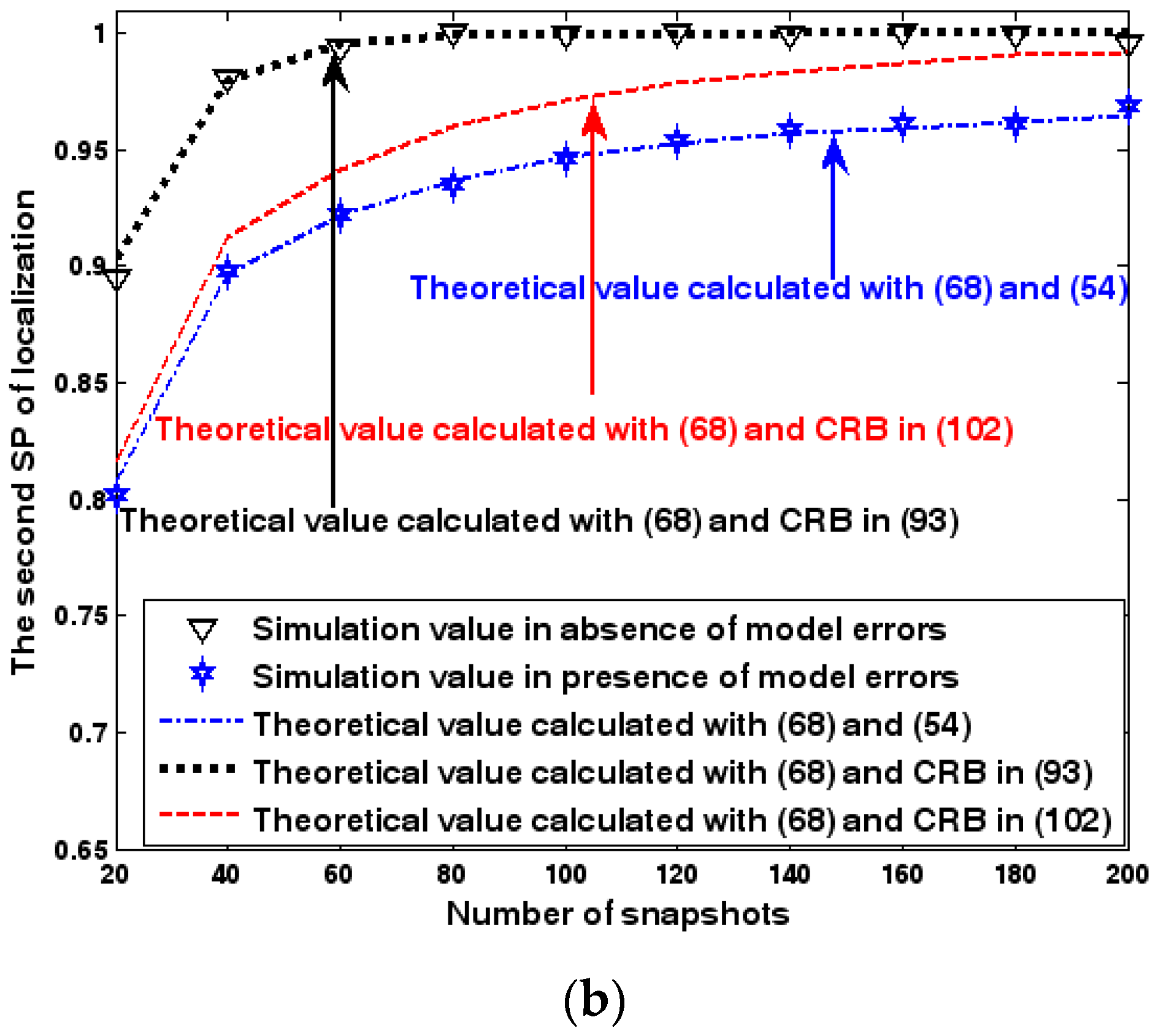
Figure 16.
SP of localization as a function of SNR of the emitter signal. (a) The first SP of localization as a function of SNR of the emitter signal. (b) The second SP of localization as a function of SNR of the emitter signal.
Figure 16.
SP of localization as a function of SNR of the emitter signal. (a) The first SP of localization as a function of SNR of the emitter signal. (b) The second SP of localization as a function of SNR of the emitter signal.

Figure 17.
SP of localization as a function of standard deviation of sensor gain perturbation. (a) The first SP of localization as a function of standard deviation of sensor gain perturbation. (b) The second SP of localization as a function of standard deviation of sensor gain perturbation.
Figure 17.
SP of localization as a function of standard deviation of sensor gain perturbation. (a) The first SP of localization as a function of standard deviation of sensor gain perturbation. (b) The second SP of localization as a function of standard deviation of sensor gain perturbation.
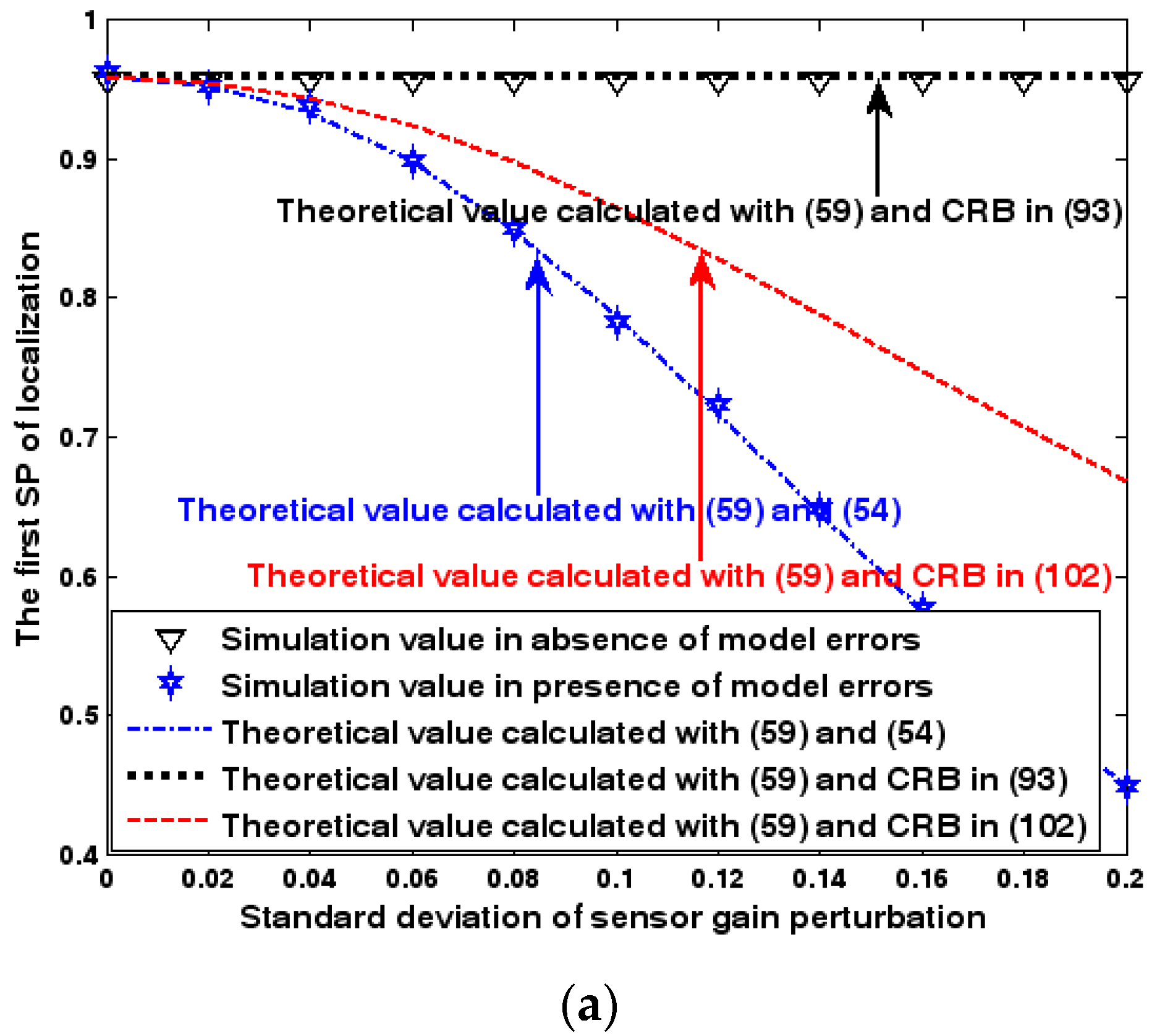

Figure 18.
SP of localization as a function of number of snapshots. (a) The first SP of localization as a function of number of snapshots. (b) The second SP of localization as a function of number of snapshots.
Figure 18.
SP of localization as a function of number of snapshots. (a) The first SP of localization as a function of number of snapshots. (b) The second SP of localization as a function of number of snapshots.

Figure 19.
Radius of CEP versus SNR of the emitter signal in the first experiment.

Figure 20.
Radius of circular error probable (CEP) versus SNR of the emitter signal in the second experiment.
Figure 20.
Radius of circular error probable (CEP) versus SNR of the emitter signal in the second experiment.


Table 1.
Notational conventions.
| Notation | Explanation |
|---|---|
| Kronecker product | |
| Schur product | |
| a diagonal matrix with diagonal entries formed from the vector | |
| a block-diagonal matrix formed from the matrices or vectors | |
| Moore-Penrose inverse of the matrix | |
| identity matrix | |
| the kth column vector of | |
| matrix of zeros | |
| vector of ones | |
| the largest eigenvalue of the matrix | |
| Euclidean norm | |
| the nth entry of the vector | |
| the nmth entry of the matrix | |
| real part of the argument | |
| imaginary part of the argument | |
| probability of the given event | |
| mathematical expectation of the random variable | |
| variance of the random variable |
© 2017 by the authors. Licensee MDPI, Basel, Switzerland. This article is an open access article distributed under the terms and conditions of the Creative Commons Attribution (CC BY) license (http://creativecommons.org/licenses/by/4.0/).
Share and Cite
MDPI and ACS Style
Wang, D.; Yu, H.; Wu, Z.; Wang, C. Performance Analysis of the Direct Position Determination Method in the Presence of Array Model Errors. Sensors 2017, 17, 1550. https://doi.org/10.3390/s17071550
AMA Style
Wang D, Yu H, Wu Z, Wang C. Performance Analysis of the Direct Position Determination Method in the Presence of Array Model Errors. Sensors. 2017; 17(7):1550. https://doi.org/10.3390/s17071550
Chicago/Turabian StyleWang, Ding, Hongyi Yu, Zhidong Wu, and Cheng Wang. 2017. "Performance Analysis of the Direct Position Determination Method in the Presence of Array Model Errors" Sensors 17, no. 7: 1550. https://doi.org/10.3390/s17071550
Note that from the first issue of 2016, this journal uses article numbers instead of page numbers. See further details here.