Dual-Channel Cosine Function Based ITD Estimation for Robust Speech Separation


Department of Electronic Engineering/Graduate School at Shenzhen, Tsinghua University, Beijing 100084, China
*
Author to whom correspondence should be addressed.
Sensors 2017, 17(6), 1447; https://doi.org/10.3390/s17061447
Submission received: 11 April 2017
/
Revised: 2 June 2017
/
Accepted: 6 June 2017
/
Published: 20 June 2017
(This article belongs to the Special Issue Recent Advances in Array Signal Processing and Its Applications in IoT Security)
Abstract
:In speech separation tasks, many separation methods have the limitation that the microphones are closely spaced, which means that these methods are unprevailing for phase wrap-around. In this paper, we present a novel speech separation scheme by using two microphones that does not have this restriction. The technique utilizes the estimation of interaural time difference (ITD) statistics and binary time-frequency mask for the separation of mixed speech sources. The novelties of the paper consist in: (1) the extended application of delay-and-sum beamforming (DSB) and cosine function for ITD calculation; and (2) the clarification of the connection between ideal binary mask and DSB amplitude ratio. Our objective quality evaluation experiments demonstrate the effectiveness of the proposed method.
1. Introduction
A common example of the well-known ‘cocktail party’ problem is the situation in which the voices of two speakers overlap. How to solve the ‘cocktail party’ problem and obtain an enhanced voice of a particular speaker in machines have grabbed serious attention of researchers.
As for single-channel speech separations, independent component analysis (ICA) [1] and nonnegative-matrix factorization (NMF) [2] are the conventional methods. However, the assumption that signals are statistically independent in ICA and the model in NMF is linear limit their applications. Moreover, NMF generally requires a large amount of computation to determine the speaker independent basis. Recently, in [3], the authors proposed an online adaptive process independent of parameter initialization, with noise reduction as a pre-processing step. Using adaptive parameters computed frame-by-frame, this article constructs a Time Frequency (TF) mask for the separation process. In [4], the authors proposed a pseudo-stereo mixture model by reformulating the binaural blind speech separation algorithm for the monaural speech separation problem. The algorithm estimates the source characteristics and constructs the masks with the parameters estimated through a weighted complex 2D histogram.
Normally, multiple channel sources are separated by measuring the differences of arrival time and sound intensity between microphones [5,6], which are also referred to as the interaural time differences (ITD) and the interaural intensity differences (IID). Interaural phase differences (IPD) have been used in [7,8]. The authors proposed a speech enhancement algorithm that utilizes phase-error based filters that depend only on the phase of the signals. Performances of the above systems depend on how the ITD (or IPD) threshold is selected. Instead of a fixed threshold, in [9], the authors employed a statistical modeling of angle distributions together with a channel weighting to determine which signal components belong to the target signal and which components are part of the background. In [10], the authors proposed a method based on a prediction of the coherence function and then estimated the signal to noise ratio (SNR) to generate Wiener filter. In [11], the author presented a method based on independent component analysis (ICA) and binary time-frequency masking. In [12], the authors proposed that a rough estimate of channel level difference (CLD) threshold yielding the best Signal-to-Distortion Ratio (SDR) could be obtained by cross-correlating the separated sounds. In addition, a combination of negative matrix factorization (NMF) with spatial localization via the generalized cross correlation (GCC) is applied for two-channel speech separation in [13]. For two-channel convolutive source separation, as the number of parameters in the NMF2D grows exponentially and the number of frequency basis increases linearly, the issues of model-order fitness, initialization and parameters estimation become even more critical. In [14], the authors proposed a Gaussian Expectation Maximization and Multiplicative Update (GEM-MU) algorithm to calculate the NMF2D with adaptive sparsity model and to utilize a Gamma-Exponential process in order to estimate the number of components and number of convolutive parameters in NMF2D.
The goal of this paper is to cope with competing-talker scenarios by dual-channel mixtures. In this study, we use DSB to generate the cosine function that evaluates ITD by using several frames of the short-time Fourier transform (STFT) and makes target and competing signals have the same characteristics. Then, we utilize the binary time-frequency mask to obtain the target source. There are two contributions in this paper:
- (1)
- we novelly upgrade delay-and-sum beamforming (DSB) [15] for estimating the ITD; and
- (2)
- for the first time, we clarify the connections between ideal binary mask and DSB amplitude ratio. The framework of our approach is illustrated in Figure 1. Moreover, our proposed algorithm can handle the problem of phase wrap-around.
The remainder of this paper is organized as follows: Section 2 provides an overview of time difference model. Our proposed approach including system overview and algorithm will be discussed in Section 3. In Section 4, we will introduce source separation. Then, Section 5 shows our evaluations of the system. Finally, Section 6 puts forward the main conclusions of the work.
2. Time Difference Model
We suppose that there are I ( sources (subscript 1 to represent the target and subscript 2 to represent the noise) in a sonic environment. The signals from two different microphones are defined, respectively, as:
where and denote the weighted coefficients of the recordings of the left and right microphone from the i-th source separately. is the time delay of arrival (TDOA) of the i-th source between two microphones. Equation (1) can be simplified as:
where is the ratio of and . By the short-time Fourier transform (STFT), the signals can be expressed as:
where m is the frame index and . k and K are the frequency index and total window length, respectively. Under the assumption of Wdisjoint orthogonal [16], Equation (3) can be rewritten as:
Thus, once the TDOA is obtained, we can make a simple binary decision concerning whether the time-frequency bin is likely to belong to the target speaker or not.
3. Proposed Approach
Delay-and-sum (DSB) is an effective means for speech enhancement. Our method is based on DSB under the anechoic condition in the time-frequency domain. In DSB, the enhanced speeches in the time-frequency domain are modeled as:
where and are the enhanced speech of target and interferer, respectively.
Theoretically, once the correct estimations of and are obtained, Equation (5) is written as:
We define as:
where
According to Equations (6) and (7), we treat as the theoretical result of . Under the assumption of far-field ( ≈ ), is simplified to
We may obtain
where is the cosine function. Specially, if equals 1, we have
Obviously, the maximum of is 1. Furthermore, we let be the real data of according to Equation (6). To ensure that the maximum of is 1, we rectify as:
We define the minimum of as . Under the correct estimations of and , approximately equals . According to Equation (10), can be estimated as:
Figure 2 demonstrates the process of ITD estimation. Figure 3 gives an example about the cosine functions with different estimations of ITD.
We define the criterion function as:
Because of the periodicity of Trigonometric function, we fix . We use the summation on all frequency bands to avoid phase wrap-around problem. Then, we have
4. Source Separation
After obtaining the ITD and attenuation coefficients (namely and ), we adopt the masking method to separate the target and competing sources. Firstly, we illustrate the effects of attenuation coefficients. Then, we utilize the time-frequency mask based on the DSB ratio.
4.1. The Effects of Weighted Coefficients
In Equation (10), we assume ≈ , but sometimes experiment settings can not meet this hypothesis strictly. In this section, we set different values of and artificially to demonstrate the effectiveness of the criterion function in Equation (14). We verify the effects of and with a simple example. Assume that
The details are shown in Figure 4. We can observe that even experiment settings do not meet the assumption that ≈ strictly, and the ITD still can be estimated accurately. Moreover, though the values of and are rough, the binary mask is free from attenuation coefficients since the DSB based mask only relies on ITD information.
4.2. Mask Based on DSB Ratio
Under the assumption of Wdisjoint orthogonal, the ideal ratio mask is defined using a priori energy ratio [17]:
In addition, the ideal binary is of the form:
where is set to be a value in –.
In our theoretical framework, is greater than 1 according to Equation (6), while is always less than 1. Then, the DSB ratio is of the form:
Comparing to 1, the binary time-frequency mask is obtained as:
It is easy to find that when is set to 0.5, is equivalent to . Equations (6) and (20) demonstrate the essence that provides the best performance under the assumption of Wdisjoint orthogonal. Then, the speech can be separated as:
where is defined as:
Finally, we can obtain the separated speech waveforms using the Inverse Fast Fourier Transform (IFFT) and OverLapping and Adding (OLA).
5. Experimental Evaluations
In this section, we first describe the experimental data and evaluation criteria that we used, and then present experimental results.
5.1. Experimental Setup
Figure 5 depicts the simulated experimental set-up. The sources are selected from the TIMIT database [18]. The sample rate of these audio files is 16,000 Hz. For simulated data, we evaluate the target speech separation performance using Perceptual Evaluation of Speech Quality (PESQ), , and [19]. These new composite measures show moderate advantages over the existing objective measures [19]. To meet the SiSEC 2010 campaign’s evaluation criteria, we adopt the standard Source-to-Interference Ratio (SIR) [20] for SiSEC 2010 test data. For these objective measures, the higher values mean better performance.
The window length is 1024 samples with an overlap of 75%. We can calculate the voiced frames detected by Voice Active Detector (VAD) [21] to avoid the situation that . Actually, hardly occurs and we do not have this operation in our experiment. Once the amplitude of is nonzero, we treat as one of the speakers.
5.2. Simulated Data
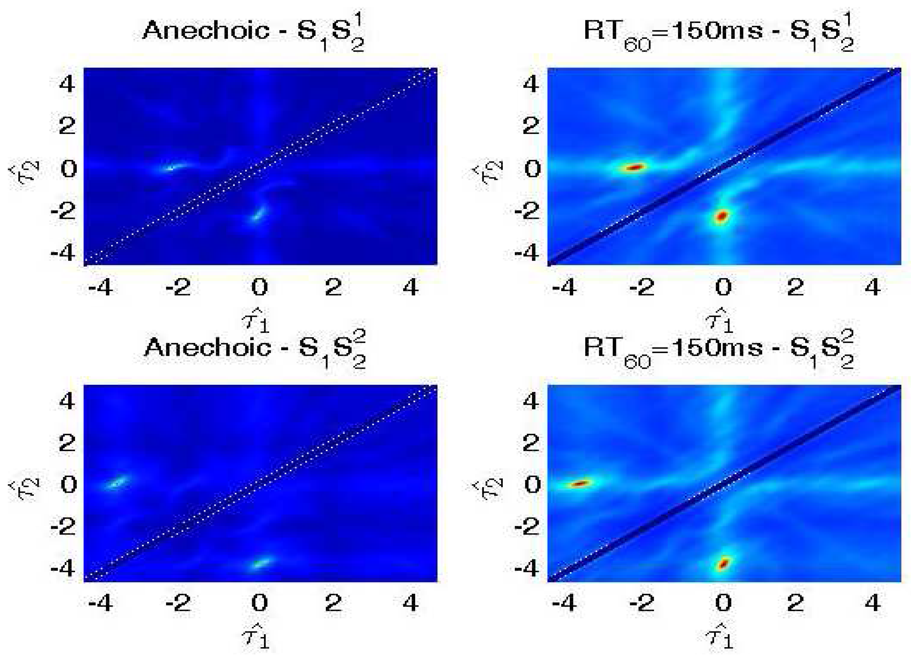
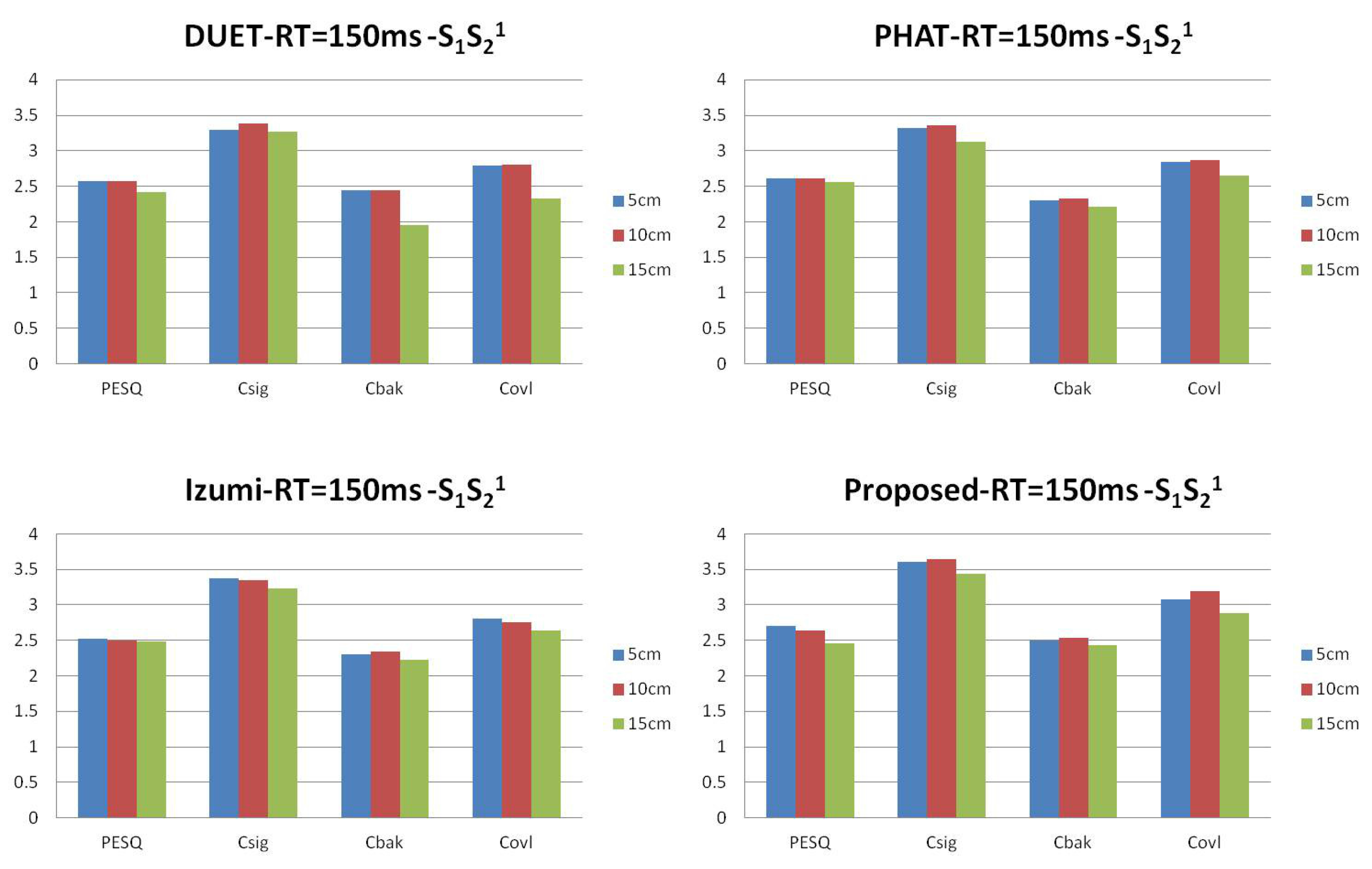
We generate data for the setup in Figure 5 with source signals of duration 2 s. Reverberation simulations are accomplished using the Room Impulse Response (RIR) open source software package [22] based on the image method. We generate 100 mixed sentences for each experimental set. Table 1 and Table 2 show the ITD estimated results in terms of mean square errors. In our experiment, the units of ITD are represented by . We compare our approach with other existing DUET [23], Messl [24], and Izumi [25] methods. Unlike the algorithms based on coherence, our method consolidates the estimation of and into one cosine function. Our method acquires better ITD estimation. Table 3 shows the relations between microphone distances with ITD estimated results. The real ITD is proportional to the distances. The estimated ITDs calculated by our method meet this rule. For all of the distances in our experiment, the proposed method provides better ITD estimations that influence the separation results. Figure 6 shows the details with ITD estimation. Though our method does not take reverberation into consideration, the results demonstrate that our method is effective for low reverberation ( = 150 ms) conditions. Figure 7 shows the target source separation performance and illustrates that our method has comparable performance. Figure 8 shows the target source separation performance for different microphone distances. For different microphone distances, the source separation performances are effective. Compared with other methods, the proposed method yields better results for all of the microphone distances.
5.3. SiSEC 2010 Test Data
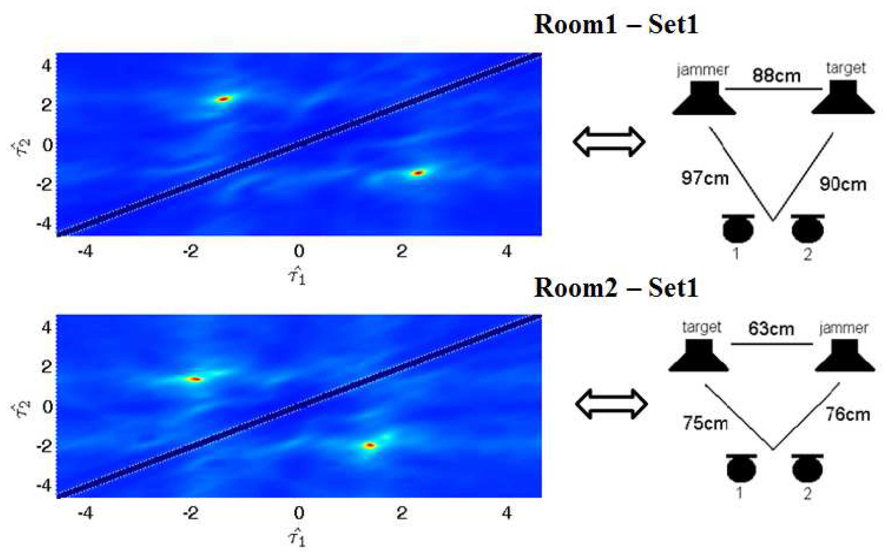
The data of D2-2 sets of the Signal Separation Evaluation Campaign (SiSEC) [26] consists of two-microphone real world recordings. We applied the proposed method to set1 for both room1 and room2. We only compare our method with the classical Fast-ICA [27], since the results with other methods can be found online. Figure 9 shows ITD estimation details. Table 1 and Table 2 illustrate that our method can achieve competitive results.
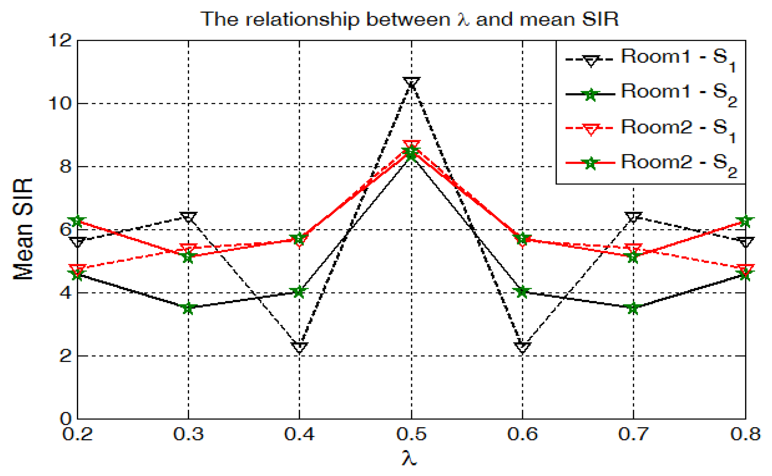
In Figure 10, we demonstrate the trends between and mean SIR for room1 and room2. Mean SIR is symmetrical to , where mean SIR achieves the best performance. These characteristics are consistent with our method.
Table 4 shows the separation performance for both room1 and room2.
6. Conclusions
In this paper, we have proposed a novel method based on DSB for dual-channel sources separation. Our method, for the first time, employs the extension of DSB for estimating interaural time difference (ITD) and illustrates the connection between ideal binary mask and DSB amplitude ratio. Our method is valid for phase wrap-around. Although our method is based on the assumption of an anechoic environment, the results illustrate the effectiveness for low reverberation environment ( = 150 ms). Objective evaluations demonstrate the effectiveness of our proposed methods.
In this paper, we focus on the estimation of the interaural time differences (ITD). In fact, the construction of an effective masking model is also very critical. We could attempt to replace our Time-Frequency Masking with an NMF2D model as proposed in [14], and adopt the GEM-MU and Gamma-Exponential process to separate sound sources. Moreover, in the presence of background noise, the idea of noise reduction in [3] is also valuable for our dual-channel speech separation.
Author Contributions
Xuliang Li performed the experiments and analyzed the data; Zhaogui Ding designed the experiments and analyzed the data; Weifeng Li and Qingmin Liao helped to discuss the results and revise the paper. All authors have read and approved the submission of the manuscript.
Conflicts of Interest
The authors declare no conflict of interest.
References
- Kouchaki, S.; Sanei, S. Supervised single channel source separation of EEG signals. In Proceedings of the 2013 IEEE International Workshop on Machine Learning for Signal Processing (MLSP), Southampton, UK, 22–25 September 2003; pp. 1–5. [Google Scholar]
- Gao, B.; Woo, W.; Dlay, S. Single-channel source separation using EMD-subband variable regularized sparse features. IEEE Trans. Audio Speech Lang. Process. 2011, 19, 961–976. [Google Scholar] [CrossRef]
- Tengtrairat, N.; Woo, W.L.; Dlay, S.S.; Gao, B. Online noisy single-channel source separation using adaptive spectrum amplitude estimator and masking. IEEE Trans. Signal Process. 2016, 64, 1881–1895. [Google Scholar] [CrossRef]
- Tengtrairat, N.; Gao, B.; Woo, W.L.; Dlay, S.S. Single-channel blind separation using pseudo-stereo mixture and complex 2D histogram. IEEE Trans. Neural Netw. Learn. Syst. 2013, 24, 1722–1735. [Google Scholar] [CrossRef] [PubMed]
- Clark, B.; Flint, J.A. Acoustical direction finding with time-modulated arrays. Sensors 2016, 16, 2107. [Google Scholar] [CrossRef] [PubMed]
- Velasco, J.; Pizarro, D.; Macias-Guarasa, J. Source localization with acoustic sensor arrays using generative model based fitting with sparse constraints. Sensors 2012, 12, 13781–13812. [Google Scholar] [CrossRef] [PubMed]
- Aarabi, P.; Shi, G. Phase-based dual-microphone robust speech enhancement. IEEE Trans. Syst. Man Cybern. Part B Cybern. 2004, 34, 1763–1773. [Google Scholar] [CrossRef]
- Kim, C.; Stern, R.M.; Eom, K.; Lee, J. Automatic selection of thresholds for signal separation algorithms based on interaural delay. Proccedings of the INTERSPEECH 2010, Chiba, Japan, 26–30 September 2010; pp. 729–732. [Google Scholar]
- Kim, C.; Khawand, C.; Stern, R.M. Two-microphone source separation algorithm based on statistical modeling of angle distributions. Proccedings of the 2012 IEEE International Conference on Acoustics, Speech and Signal Processing (ICASSP), Kyoto, Japan, 25–30 March 2012; pp. 4629–4632. [Google Scholar]
- Yousefian, N.; Loizou, P.C. A dual-microphone algorithm that can cope with competing-talker scenarios. IEEE Trans. Audio Speech Lang. Process. 2013, 21, 145–155. [Google Scholar] [CrossRef]
- Pedersen, M.S.; Wang, D.; Larsen, J.; Kjems, U. Two-microphone separation of speech mixtures. IEEE Trans. Neural Netw. 2008, 19, 475–492. [Google Scholar] [CrossRef] [PubMed]
- Nishiguchi, M.; Morikawa, A.; Watanabe, K.; Abe, K.; Takane, S. Sound source separation and synthesis for audio enhancement based on spectral amplitudes of two-channel stereo signals. J. Acoust. Soc. Am. 2016, 140, 3428. [Google Scholar] [CrossRef]
- Wood, S.; Rouat, J. Blind speech separation with GCC-NMF. In Proceedings of the INTERSPEECH 2016, San Francisco, CA, USA, 8–12 September 2016. [Google Scholar]
- Al-Tmeme, A.; Woo, W.L.; Dlay, S.S.; Gao, B.; Al-Tmeme, A.; Woo, W.L.; Dlay, S.S.; Gao, B.; Woo, W.L.; Dlay, S.S.; et al. Underdetermined Convolutive Source Separation Using GEM-MU With Variational Approximated Optimum Model Order NMF2D. IEEE/ACM Trans. Audio Speech Lang. Process. (TASLP) 2017, 25, 35–49. [Google Scholar] [CrossRef]
- Brandstein, M.; Ward, D. Microphone Arrays: Signal Processing Techniques and Applications; Springer: Berlin, Germany, 2001. [Google Scholar]
- Yilmaz, O.; Rickard, S. Blind separation of speech mixtures via time-frequency masking. IEEE Trans. Signal Process. 2004, 52, 1830–1847. [Google Scholar] [CrossRef]
- Srinivasan, S.; Roman, N.; Wang, D. Binary and ratio time-frequency masks for robust speech recognition. Speech Commun. 2006, 48, 1486–1501. [Google Scholar] [CrossRef]
- Zue, V.; Seneff, S.; Glass, J. Speech database development at MIT: TIMIT and beyond. Speech Commun. 1990, 9, 351–356. [Google Scholar] [CrossRef]
- Hu, Y.; Loizou, P.C. Evaluation of objective quality measures for speech enhancement. IEEE Trans. Audio Speech Lang. Process. 2008, 16, 229–238. [Google Scholar] [CrossRef]
- Vincent, E.; Sawada, H.; Bofill, P.; Makino, S.; Rosca, J.P. First stereo audio source separation evaluation campaign: Data, algorithms and results. In Independent Component Analysis and Signal Separation; Springer: Heidelberg, Germany, 2007; pp. 552–559. [Google Scholar]
- Cho, Y.D.; Kondoz, A. Analysis and improvement of a statistical model-based voice activity detector. IEEE Signal Process. Lett. 2001, 8, 276–278. [Google Scholar]
- Allen, J.B.; Berkley, D.A. Image method for efficiently simulating small-room acoustics. J. Acoust. Soc. Am. 1979, 65, 943–950. [Google Scholar] [CrossRef]
- Wang, Y.; Yılmaz, Ö.; Zhou, Z. Phase aliasing correction for robust blind source separation using DUET. Appl. Comput. Harmonic Anal. 2013, 35, 341–349. [Google Scholar] [CrossRef]
- Mandel, M.; Weiss, R.J.; Ellis, D.P. Model-based expectation-maximization source separation and localization. IEEE Trans. Audio Speech Lang. Process. 2010, 18, 382–394. [Google Scholar] [CrossRef]
- Izumi, Y.; Ono, N.; Sagayama, S. Sparseness-based 2ch BSS using the EM algorithm in reverberant environment. In Proceedings of the 2007 IEEE Workshop on Applications of Signal Processing to Audio and Acoustics, New Paltz, NY, USA, 21–24 October 2007; pp. 147–150. [Google Scholar]
- Araki, S.; Theis, F.; Nolte, G.; Lutter, D.; Ozerov, A.; Gowreesunker, V.; Sawada, H.; Duong, N.Q.K. The 2010 Signal Separation Evaluation Campaign (SiSEC2010): Audio Source Separation. Lect. Notes Comput. Sci. 2010, 6365, 414–422. [Google Scholar]
- Koldovsky, Z.; Tichavsky, P.; Oja, E. Efficient Variant of Algorithm FastICA for Independent Component Analysis Attaining the Cram—Rao Lower Bound. IEEE Trans. Neural Netw. 2006, 17, 1265–1277. [Google Scholar] [CrossRef] [PubMed]
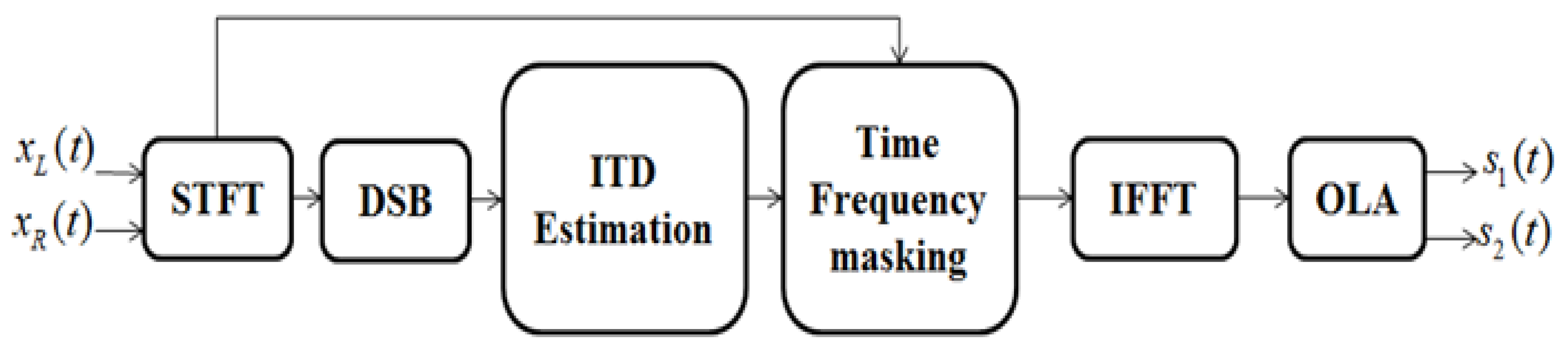
Figure 1.
Block diagram of the proposed approach. STFT: Short Time Fourier Transform, DSB: Delay-and-Sum Beamforming, ITD: Interaural Time Difference, IFFT: Inverse Fast Fourier Transform, OLA: OverLapping and Adding.
Figure 1.
Block diagram of the proposed approach. STFT: Short Time Fourier Transform, DSB: Delay-and-Sum Beamforming, ITD: Interaural Time Difference, IFFT: Inverse Fast Fourier Transform, OLA: OverLapping and Adding.

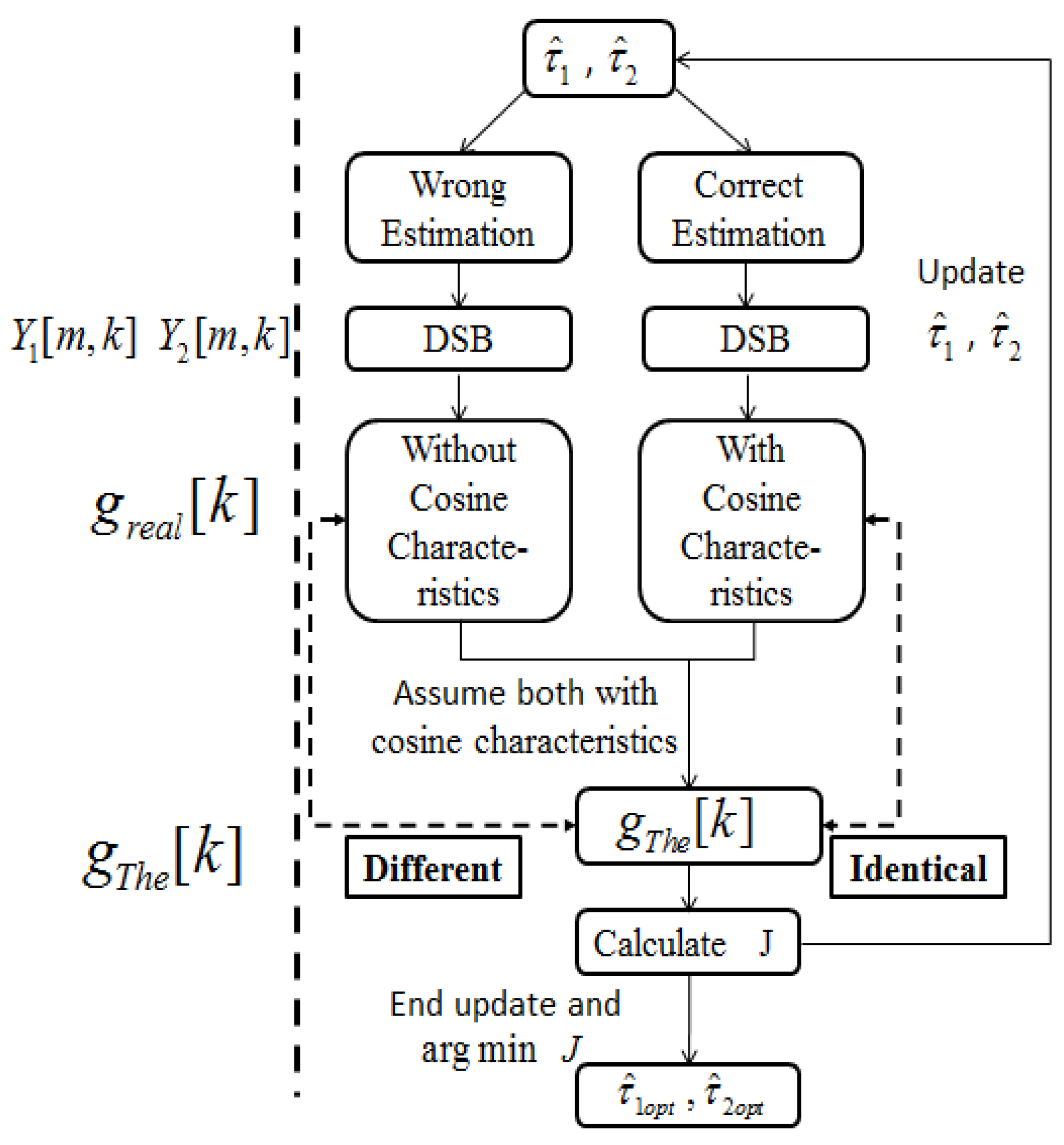
Figure 2.
Float chart of ITD estimation. and are the estimation values of and . If correct estimations of and are obtained, the cosine characteristics of is identical to . In spite of the fact that there would be no cosine characteristics in based on incorrect estimation results, we can still follow the cosine characteristics to calculate . Obviously, is different to in this situation. We find the true value of and iteratively. The and will be updated until is identical to .

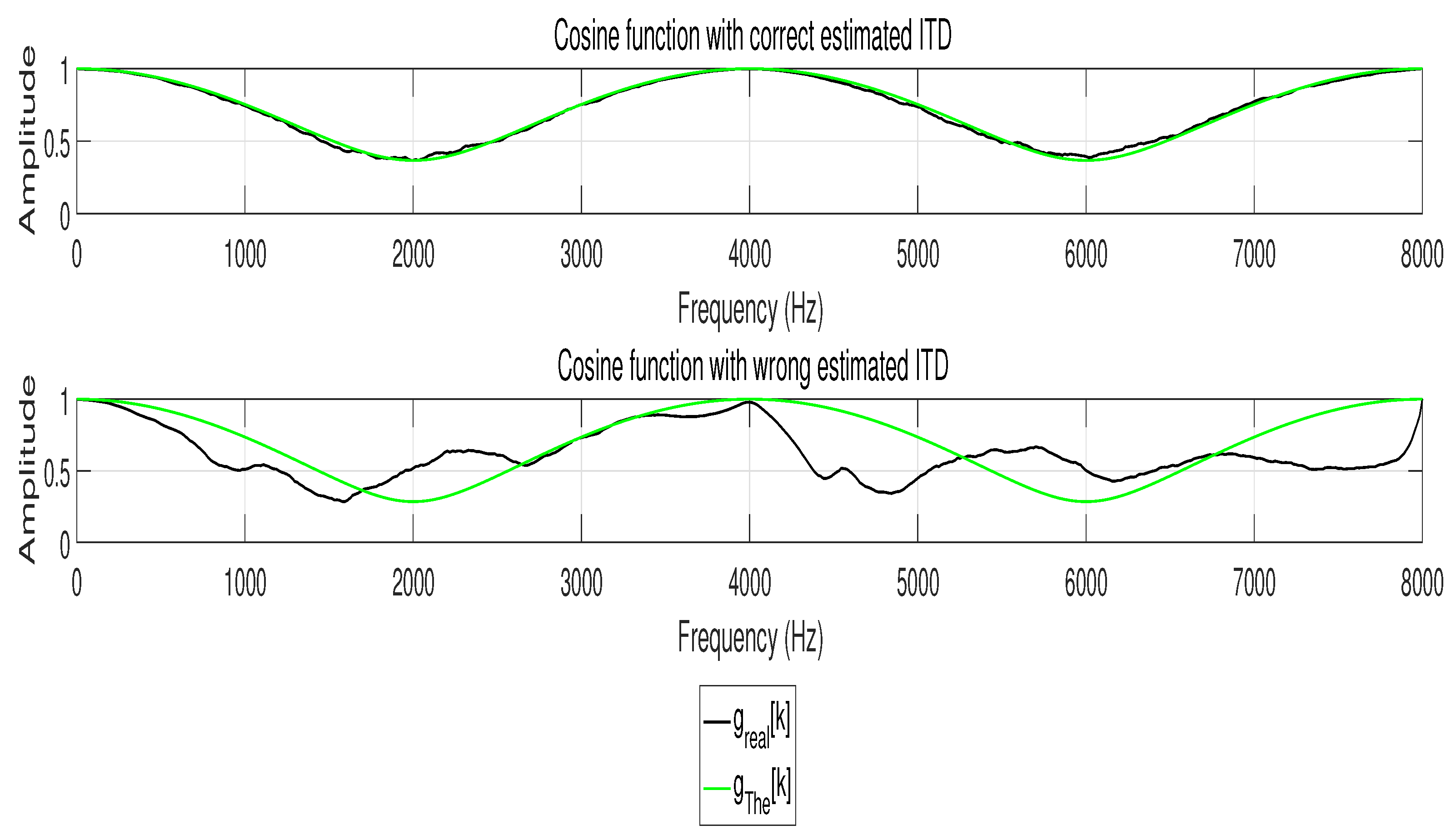
Figure 3.
Cosine function with different ITD estimation. Obviously, is identical to with correct ITD estimation, while is different to with incorrect ITD estimation.
Figure 3.
Cosine function with different ITD estimation. Obviously, is identical to with correct ITD estimation, while is different to with incorrect ITD estimation.

Figure 4.
Source localization with different and . The source localization are conducted in four different settings: (1) , ; (2) , ; (3) , ; and (4) , . The ITD estimation is valid for all of the settings.
Figure 4.
Source localization with different and . The source localization are conducted in four different settings: (1) , ; (2) , ; (3) , ; and (4) , . The ITD estimation is valid for all of the settings.
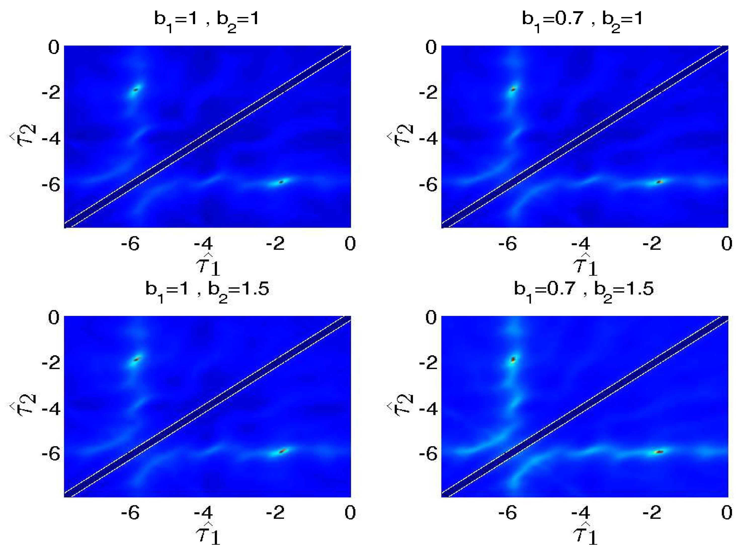
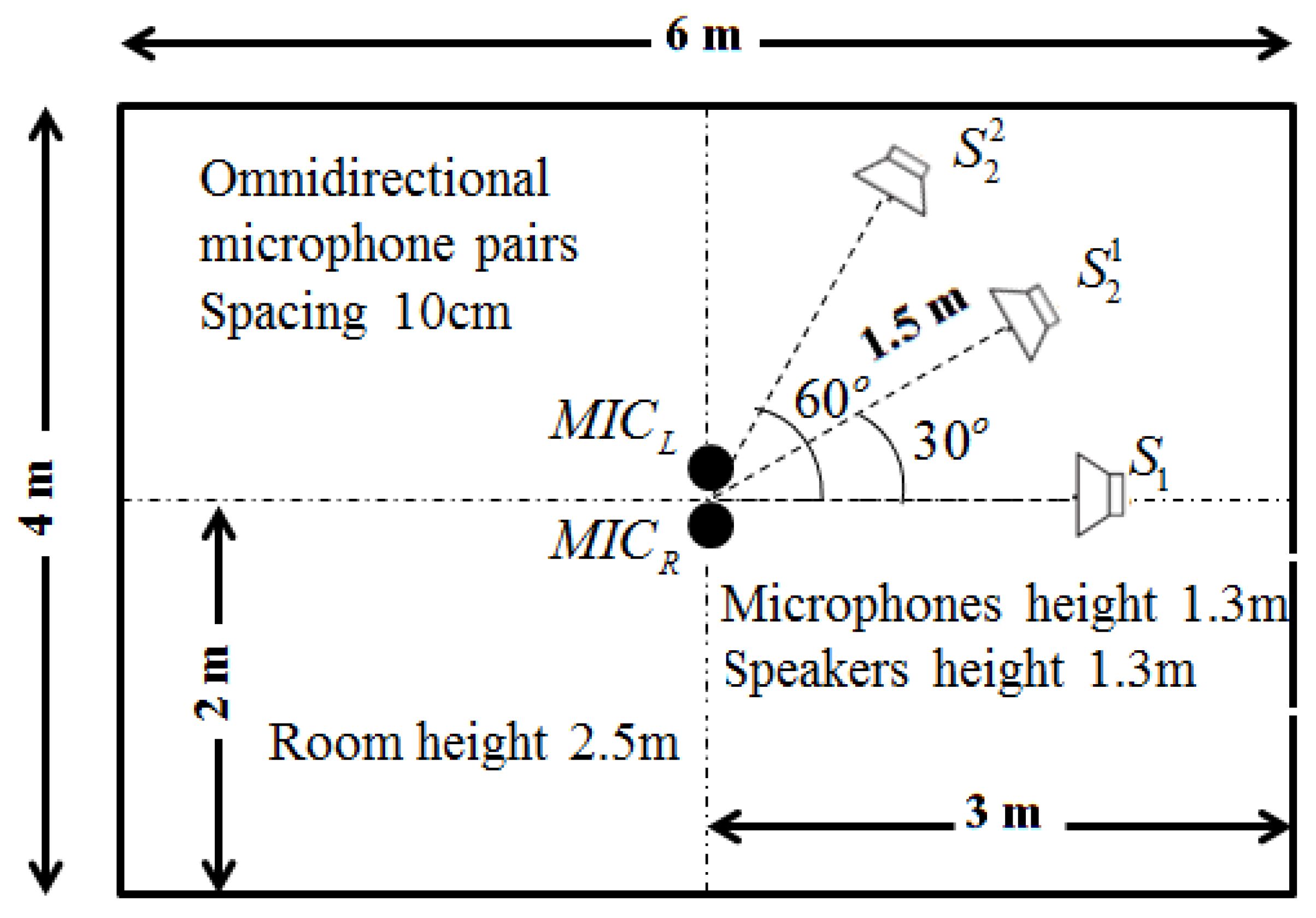
Figure 5.
Placement of the microphones and sound sources. is the target source. and are the competing sources in two different environments, respectively.
Figure 5.
Placement of the microphones and sound sources. is the target source. and are the competing sources in two different environments, respectively.

Figure 6.
ITD estimation results in different environments. The horizontal coordinate corresponds to , and the vertical coordinate corresponds to . In fact, we can only process the lower triangular matrix because the estimations have symmetric properties.
Figure 6.
ITD estimation results in different environments. The horizontal coordinate corresponds to , and the vertical coordinate corresponds to . In fact, we can only process the lower triangular matrix because the estimations have symmetric properties.

Figure 7.
The target speech performance of different methods in terms of Perceptual Evaluation of Speech Quality (PESQ), , and .
Figure 7.
The target speech performance of different methods in terms of Perceptual Evaluation of Speech Quality (PESQ), , and .
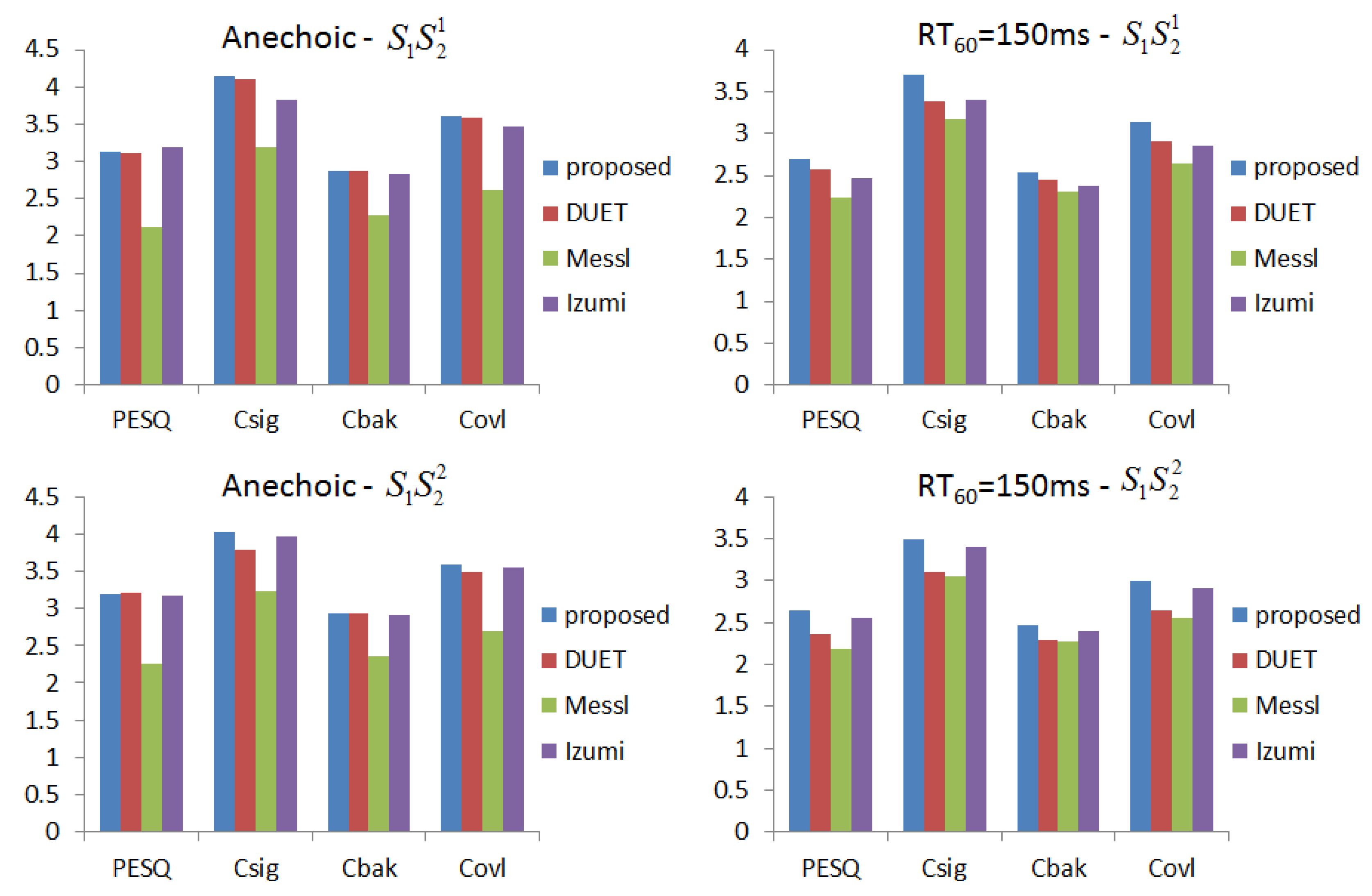
Figure 8.
The target speech performance of different microphone distances in terms of Perceptual Evaluation of Speech Quality (PESQ), , and .
Figure 8.
The target speech performance of different microphone distances in terms of Perceptual Evaluation of Speech Quality (PESQ), , and .

Figure 9.
ITD estimation results and experimental set-up in room1 and room2. The horizontal coordinate corresponds to , and the vertical coordinate corresponds to . The distance between two microphones is 8 cm.
Figure 9.
ITD estimation results and experimental set-up in room1 and room2. The horizontal coordinate corresponds to , and the vertical coordinate corresponds to . The distance between two microphones is 8 cm.

Figure 10.
Average Signal-to-Interference Ratio (SIR) with different . We calculate the mean of SIR for each . The result demonstrates that provides the best performance, which is identical to our theoretical analysis. Furthermore, separation results are symmetrical to when we adopt the signal-to-noise ratio based on and to generate the ideal binary mask.

Table 1.
ITD estimation on .
| Anechoic | = 150 ms | ||||
|---|---|---|---|---|---|
| Method | Method | ||||
| Real ITD | 0.000 | 2.373 | Real ITD | 0.000 | 2.373 |
| DUET | 0.058 | 2.370 | DUET | 0.520 | 2.560 |
| Phat | 0.017 | 2.502 | Phat | 0.217 | 2.500 |
| Izumi | 0.093 | 2.502 | Izumi | 0.337 | 2.946 |
| Proposed | 0.024 | 2.402 | Proposed | 0.179 | 2.428 |
Table 2.
Interaural Time Difference (ITD) estimation on .
| Anechoic | = 150 ms | ||||
|---|---|---|---|---|---|
| Method | Method | ||||
| Real ITD | 0.000 | 4.060 | Real ITD | 0.000 | 4.060 |
| DUET | 0.020 | 3.963 | DUET | 1.844 | 3.448 |
| Phat | 0.055 | 4.009 | Phat | 0.117 | 4.122 |
| Izumi | 0.045 | 4.018 | Izumi | 0.043 | 4.067 |
| Proposed | 0.012 | 4.039 | Proposed | 0.042 | 4.045 |
Table 3.
ITD estimation on = 150 ms with different microphone distances.
| Mic-Distance | 5 cm | 10 cm | 15 cm | |||
|---|---|---|---|---|---|---|
| Method | ||||||
| Real ITD | 0.000 | 1.187 | 0.000 | 2.373 | 0.000 | 3.560 |
| DUET | 0.271 | 1.069 | 0.520 | 2.560 | 1.678 | 3.135 |
| PHAT | 0.163 | 1.296 | 0.217 | 2.500 | 0.126 | 3.652 |
| Izumi | 0.234 | 1.334 | 0.337 | 2.946 | 0.031 | 3.891 |
| Proposed | 0.112 | 1.125 | 0.179 | 2.428 | 0.041 | 3.527 |
Table 4.
Signal-to-Interference Ratio (SIR) evaluations based on room1 and room2.
| Room1 | x1 | x2 | x3 | x4 | x5 | x6 | |
| Proposed | 11.8 | 7.8 | 14.7 | 26.4 | 4.9 | ||
| 10.5 | 12.2 | 2.7 | 14.0 | 21.2 | |||
| ICA | 0.3 | 10.2 | 18.6 | ||||
| 3.3 | 4.8 | 10.0 | 18.3 | ||||
| Room2 | x1 | x2 | x3 | x4 | x5 | x6 | |
| Proposed | 3.3 | 6.2 | 12.3 | 27.5 | 3.2 | 1.0 | |
| 12.8 | 11.1 | 15.8 | 22.5 | ||||
| ICA | 6.6 | 19.6 | |||||
| 6.2 | 4.8 | 12.0 | 19.4 | ||||
1 The definition of ICA is “Independent Component Analysis”.
© 2017 by the authors. Licensee MDPI, Basel, Switzerland. This article is an open access article distributed under the terms and conditions of the Creative Commons Attribution (CC BY) license (http://creativecommons.org/licenses/by/4.0/).
Share and Cite
MDPI and ACS Style
Li, X.; Ding, Z.; Li, W.; Liao, Q. Dual-Channel Cosine Function Based ITD Estimation for Robust Speech Separation. Sensors 2017, 17, 1447. https://doi.org/10.3390/s17061447
AMA Style
Li X, Ding Z, Li W, Liao Q. Dual-Channel Cosine Function Based ITD Estimation for Robust Speech Separation. Sensors. 2017; 17(6):1447. https://doi.org/10.3390/s17061447
Chicago/Turabian StyleLi, Xuliang, Zhaogui Ding, Weifeng Li, and Qingmin Liao. 2017. "Dual-Channel Cosine Function Based ITD Estimation for Robust Speech Separation" Sensors 17, no. 6: 1447. https://doi.org/10.3390/s17061447
Note that from the first issue of 2016, this journal uses article numbers instead of page numbers. See further details here.