
An Exact Model-Based Method for Near-Field Sources Localization with Bistatic MIMO System


Institute of Electronics and Telecommunications of Rennes (IETR), UMR CNRS 6164, Polytech Nantes, Rue Christian Pauc, BP 50609, 44306 Nantes CEDEX 3, France
*
Author to whom correspondence should be addressed.
Sensors 2017, 17(4), 723; https://doi.org/10.3390/s17040723
Submission received: 4 January 2017
/
Revised: 8 March 2017
/
Accepted: 28 March 2017
/
Published: 30 March 2017
(This article belongs to the Section Physical Sensors)
Abstract
:In this paper, we propose an exact model-based method for near-field sources localization with a bistatic multiple input, multiple output (MIMO) radar system, and compare it with an approximated model-based method. The aim of this paper is to propose an efficient way to use the exact model of the received signals of near-field sources in order to eliminate the systematic error introduced by the use of approximated model in most existing near-field sources localization techniques. The proposed method uses parallel factor (PARAFAC) decomposition to deal with the exact model. Thanks to the exact model, the proposed method has better precision and resolution than the compared approximated model-based method. The simulation results show the performance of the proposed method.
1. Introduction
Sources localization has been an important field of research for several decades. It is widely used in radar, underwater sources localization, acoustics, medicine, robotics, etc. The sources can be classified as near and far fields. Because of the wide range of applications, most of the research works [1,2,3,4,5] are dedicated to far-field sources localization. However, near-field sources localization has some important applications, like airport security control, ground penetration radar, phonocardiography, and many more.
Most of the existing near-field sources localization techniques [6,7,8,9,10,11,12,13,14,15,16] are based on an approximated model. In practice, a near-field point source has a spherical wavefront [6], which implies a nonlinear model. The wavefront of a near-field source is usually approximated as quadric (quadratic surface) to reduce the complexity of the model [6,9]. However, the use of this approximation results in a systematic error, which inevitably deteriorates the accuracy of the estimation. The systematic error is like an offset added to the actual source position, which increases when the target gets close to the antenna array [6].
In recent years, multiple input, multiple output (MIMO) radar has drawn a lot of attention. The advantages and limitations of MIMO radar have been well summarized in [2,3]. Based on the placement and configuration of the antennas, MIMO radar systems can broadly be classified as distributed or colocated. MIMO radar with colocated antennas can further be classified as monostatic, bistatic, and multistatic. In a bistatic MIMO radar system, the transmitting and receiving arrays are separated by a large distance, but the antennas in each array are kept close to each other (colocated) as compared to the distances between targets and the arrays. When the same array is used as transmitter and receiver, the system is monostatic. The directions of arrival and departure are different in the case of a bistatic MIMO system, but are equal for a monostatic MIMO radar system. If the distance between the transmitting and receiving arrays of a bistatic MIMO system is negligible compared to the range of targets, it can be considered as a pseudo-monostatic MIMO system. The work by Guo et al. [10] provides a subspace-based near-field sources localization method for a pseudo-monostatic MIMO radar system. A near-field sources localization method based on an approximated model with a bistatic MIMO system was proposed in [15]. Recently, in [17], a method based on the exact model of the received signal has been proposed to locate near-field targets using a bistatic MIMO system composed of linearly-aligned transmitting and receiving arrays. This paper is an improvement and an extension of the method in [17]. The major differences between the two are:
- The method in [17] is specific to the linearly-aligned transmitting and receiving arrays, whereas this paper deals with any configuration for the transmitting and receiving uniform linear arrays (ULAs) (3D situation).
- Due to the linearly-aligned transmitting and receiving arrays, the cost function in [17] has only two variables. However, the generalized 3D configuration in this paper results in a three-variable cost function which is much more difficult to deal with. Thus, in this paper, we propose a better and more efficient approach based on an overdetermined system of linear equations.
In [15], four parameters—namely, the angle of arrival, the angle of departure of a target, and the distances (ranges) from the target to the transmitting and receiving arrays—are used to localize the target, but there are some redundancies because three coordinates are sufficient to define the position of a target. Therefore, in this paper, we use Cartesian coordinates to formulate the signal model and express the localization error.
There are many existing methods to localize sources from an array of sensors, such as Capon’s method, multiple signal classification (MUSIC), estimation of signal parameter via rotational invariance techniques (ESPRIT), propagator method, and tensor decomposition method [1,5]. Among the methods listed above, the tensor decomposition method directly estimates the whole directional matrix instead of the directional parameters [18], which facilitates the estimation of the directional parameters from a nonlinear model such as the exact model in near-field situation. Consequently, the proposed exact model-based method uses the tensor decomposition. Tensor-based models and techniques are well adapted to MIMO radar because tensors allow coping with large systems (three or more dimensions). The received signal in the case of a bistatic MIMO system can be organized as a three-way tensor. Three-way tensors have attracted a lot of attention because they are the simplest form of tensor after a matrix and can be decomposed into unique factors, contrary to a matrix. Kruskal [19] provides a detailed study of the rank and uniqueness in the decomposition of a three-way tensor. The tensor decomposition has already been used for multiple far-field sources localization with bistatic MIMO radar [5].
There exist many tensor decomposition techniques, such as Tucker, parallel factor analysis (PARAFAC), and block component decomposition [20]. PARAFAC is often used in array signal processing thanks to its uniqueness in the decomposition of tensors under some mild conditions [18]. Thus, in this paper, we select PARAFAC to decompose the three-way tensor of the received signal to obtain the directional matrices of arrival and departure. From the existing work on the application of PARAFAC to the localization of targets, we can observe that it is mainly proposed for far-field target localization. In this paper, we extend it to the near-field situation. Once the directional matrices are estimated, an optimization method can be used to obtain the directional parameters.
To summarize, this paper focuses on the use of an exact model of the received signals of near-field sources to get better performance than the existing approximated model-based techniques for near-field sources localization with a bistatic MIMO system. Due to the nonlinear nature of the exact model, the PARAFAC decomposition is used, and an optimization technique is developed to efficiently solve this problem.
The remainder of the paper is organized as follows. In Section 2, a detailed signal model is constructed for a bistatic MIMO radar system based on the spherical wavefront of an incoming wave by taking the exact propagation model in the near-field situation into account. Section 3 provides a short presentation of the method proposed in [15]. In Section 4, the proposed method is described. Finally, some simulation results are presented to compare the performance of the proposed method with the method presented in [15], followed by some discussion and conclusions.
Notations
In the following, a bold lower case character (e.g., ) represents a vector, whereas a bold upper case character (e.g., ) denotes a matrix. A tensor is denoted by a bold upper case calligraphic font (e.g., ). , , and represent, respectively, the transpose, left pseudo-inverse, and Frobenius norm of a matrix or vector. ⊡ is the Khatri–Rao (column-wise Kronecker) product operator. The cardinal number of a set is represented by . stands for the principal value of the angle (or argument) of a complex number. represents the diagonal matrix with all the components of vector as its diagonal elements. is the expected value.
2. Signal Model
Let P be the number of narrow-band stationary point sources in the near-field region of a bistatic MIMO system with ULAs. In the following, M and N represent, respectively, the number of antennas in the transmitting and receiving arrays of the bistatic MIMO system.
For such a bistatic MIMO system, the L samples of the received matched signal in the presence of P stationary point sources can be written as [4]
where and contain the directional vectors of departure and arrival, respectively, is the matrix of the complex-valued reflection coefficients of targets, and is an additive noise matrix composed of spatially- and temporally-independent elements, and each element is a zero mean Gaussian random variable with variance . The reflection coefficients are assumed to be different for each target and randomly changing with each sample. In other words, we consider a Swerling model II case, which makes a full rank matrix [21]. The pth columns of and —denoted by and , respectively—are given by
and
where and are the indexes of the reference elements of the transmitting and receiving arrays, respectively, , and . and are the relative indexes of the respective arrays. is the wavelength of the carrier. is the difference between the distance traveled by the transmitted signal from the mth transmitting antenna to the pth target and the distance traveled by the transmitted signal from the 0th transmitting antenna to the pth target, which can be expressed as
where and are respectively the range and angle of departure of the pth target with respect to the reference transmitting antenna indexed by , and is the inter-element spacing in the transmitting array. Similarly, is the difference between the distance traveled by the reflected signal from the pth target to the nth receiving antenna and the distance traveled by the reflected signal from the pth target to the 0th receiving antenna, which can be expressed as
where and are, respectively, the range and angle of arrival of the pth target with respect to the reference receiving antenna indexed by and is the inter-element spacing in the receiving array [6].
in Equation (1) can be considered as a block matrix, . The mth sub-matrix of (i.e., ) can be expressed as
where and is the corresponding noise sub-matrix.
3. Approximated Model-Based Method Proposed in [15]
Most of the existing near-field sources localization techniques [6,7,8,9,11,14] use an approximated model, and ULA is often used in the approximated model-based methods. The approximated path differences—which are the second-order Taylor approximations of Equations (4) and (5)—can respectively be written as [6]
and
In [15], a subspace-based method is used to estimate four parameters: two ranges ( and ) and two directional angles ( and ) of a near-field target by using a bistatic MIMO system with inter-element spacing of in each ULA. , , , , , and are the necessary conditions of [15].
In an approximated model-based method like [15], and are assumed to be constructed by and , respectively. Therefore, in this case, in Equation (6) can be expressed as
where and . In [15], four cross-covariance matrices between for and are constructed. The eigenvalues of and are used to get and , and their eigenvectors are used to obtain and , where . More details can be found in [15].
4. Proposed Exact Model-Based Position Estimation Method
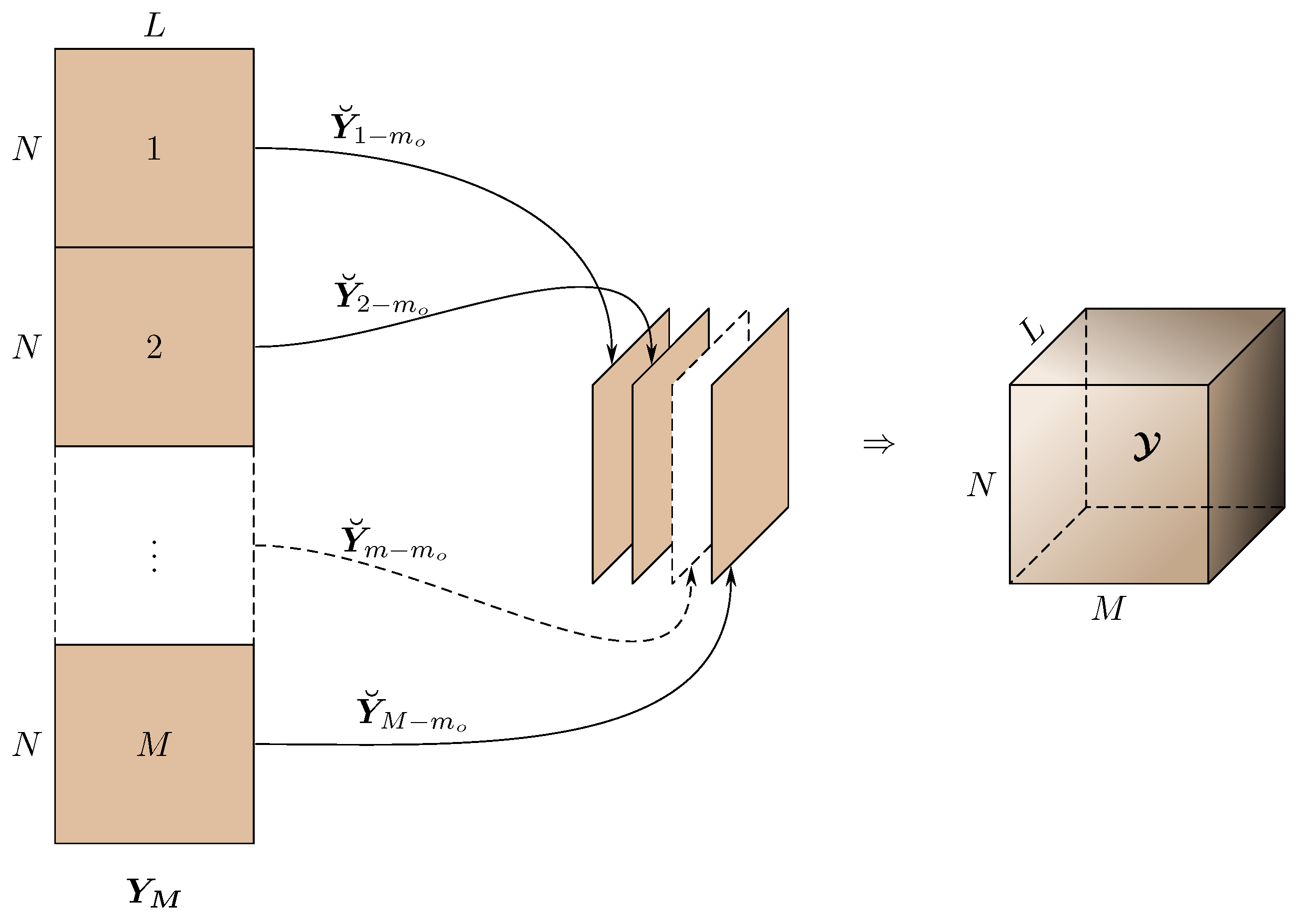
Every element of in Equation (1) is associated with three parameters related, respectively, to the receiving antenna, transmitting antenna, and time sample. Therefore, can be rearranged like a three-way tensor , as shown in Figure 1. Creating a tensor out of lower dimensional data is known as tensorization [20].
PARAFAC decomposition of tensor is used to get the estimates of , , and matrices [5]. Tensor operations are usually performed in its equivalent matrix form [5,22,23]. The process of creating a matrix out of a tensor is known as matricization [20]. Like , can be matricized into the following two additional matrices
and
According to the least squares principle, the following objective functions can be written from Equations (1), (10) and (11)
and
where , , and denote the estimated values of , , and respectively.
The trilinear alternating least squares (TALS) algorithm is a classical method to minimize the above objective functions [5,22,23]. Least squares estimates of Equations (12)–(14) are given by
and
In the TALS algorithm, Equations (15)–(17) are alternatively updated with the new values of , , and until a stopping criteria is met. is often used as the stopping condition, where is the tolerance. In practice, the algorithm given in [24] is used for PARAFAC decomposition, which uses compression, line search, normalization, etc. to accelerate the TALS method.
According to [19], the matrices obtained by PARAFAC decomposition of a three-way tensor are scaled and permuted. The permutation has no impact because the matrices’ columns are paired. However, in the proposed method, the scaling factor must be removed by dividing all the elements of the directional vectors with their corresponding reference elements.
To define the Cartesian coordinates of a target, let us assume a general configuration of bistatic MIMO system as shown in Figure 2. In the case of a ULA, the unit vector along the array and the position vector of the reference antenna of the corresponding array are sufficient to obtain the position vectors of the remaining antennas of that array. In the figure, and are the position vectors of the reference transmitting and receiving antennas, respectively, with respect to the origin of the Cartesian coordinate system, and and are the unit vectors along the transmitting and receiving arrays, respectively. represents the position vector of the pth target. In 3D space, the range and directional angle of a target with respect to a linear array make a circle related to the base of a cone with the range as its slant height and the directional angle as its half angle. In the bistatic case, we have two such circles (shown in Figure 2). The target is located at the intersection of these two circles. In the figure, and are unit vectors on the planes of the respective circles. The parametric equations of the circles can be written as
and
where × denotes the cross-product operation between two vectors; and are the position vectors of a point on the respective circles at and , respectively. The equation parameters and independently vary from 0 to rad to completely sweep the respective circles.
The ranges and directional angles can be expressed in terms of the Cartesian coordinates as , , , and . Thus, according to Equations (2)–(5), and can respectively be determined by as
and
Then, a direct approach to estimate could be the minimization of the following cost function
where and are the estimated directional vectors obtained from the PARAFAC decomposition, and and are their respective reference elements used here to remove the scaling factor in the decomposition of the received signal tensor.
Even though a near-field region occupies a finite space, minimizing Equation (22) by using grid search or Newton’s method is computationally expensive. Therefore, we choose an indirect method in which we estimate the ranges and directional angles, followed by the estimation of the coordinates.
Rearranging Equations (4) and (5), we can obtain
where and are the estimated path differences which can be directly obtained from the estimated directional vectors as follows
and
where represents the unwrapped value of the argument [25]. Equations (25) and (26) can be described as follows:
- Get the directional vectors and from the PARAFAC decomposition.
- Extract the arguments of all the components of and .
- Unwrap the phase vectors obtained from Step 2.
- Subtract the unwrapped phase corresponding to and from all the components of the unwrapped phase vector of and , respectively.
- Divide each component of the normalized phase vectors obtained from the above step by to get and .
In practice, and ; therefore, Equations (23) and (24) can be considered as an overdetermined system of linear equations in and and and , respectively, which can be solved by the total least squares method [26]. Let be the right-singular-vector associated with the smallest singular value of the following matrix formed by the coefficients of Equation (23)
The estimated range and angle of departure can respectively be computed by and . Similarly, let be the right-singular-vector associated with the smallest singular value of the following matrix formed by the coefficients of Equation (24)
The estimated range and angle of arrival can respectively be computed by and .
The estimated ranges and directional angles can be used in Equations (18) and (19) to construct the parametric equations of the circles. As mentioned before, the required coordinates are at the intersection of these circles. However, due to the estimation error and noise, the circles may not intersect; thus, the following minimization problem can be solved:
A coarse solution of Equation (29) can be calculated by exhaustive grid search, and then it can be finely tuned by Newton’s method. Solving Equation (29) is less complex than solving Equation (22). Finally, the position vector of the pth target can be computed as , , or the average of these two position vectors.
Algorithm 1 provides a summary of the proposed method.
| Algorithm 1 Algorithm of the proposed method. |
|
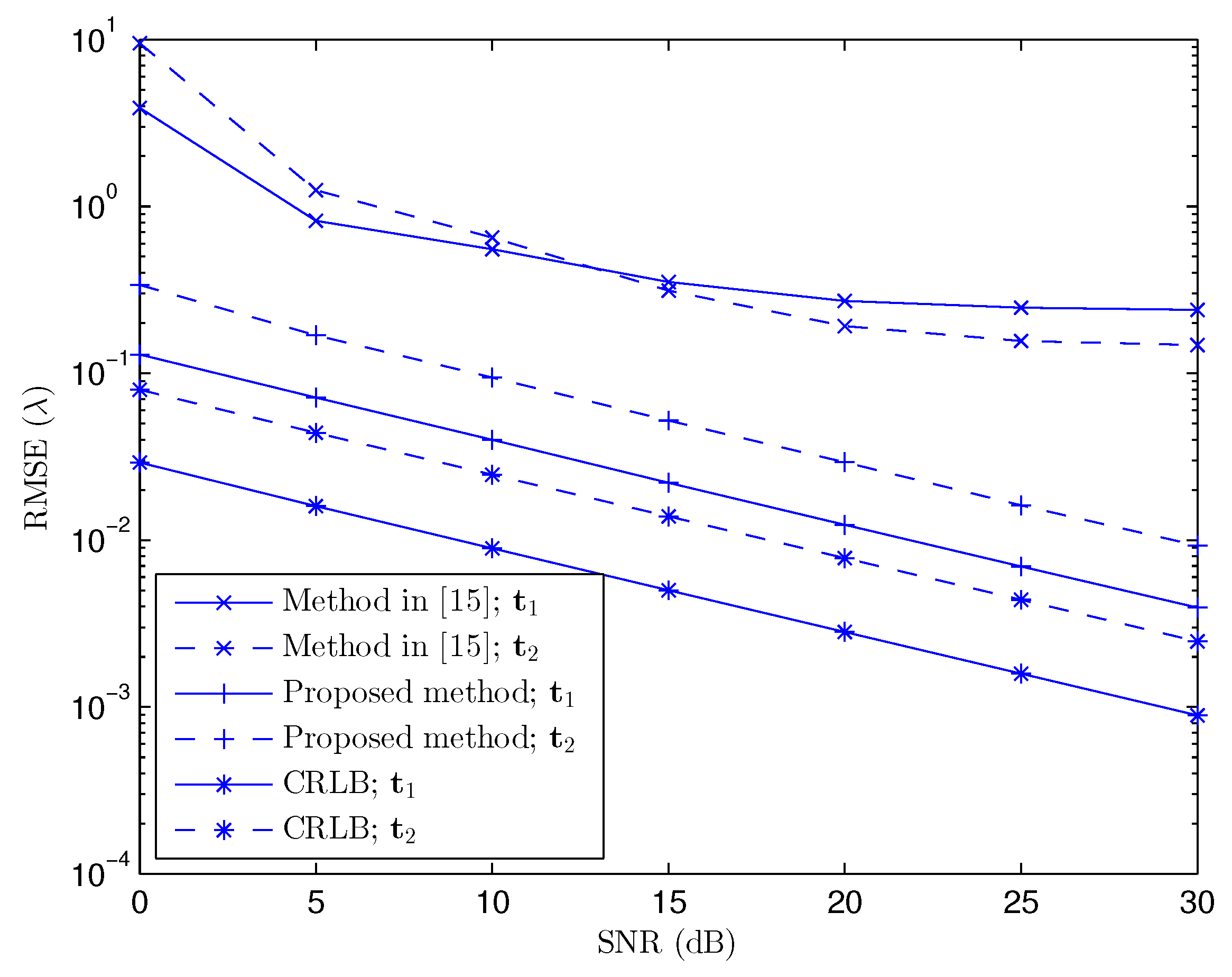
5. Simulation Results
In the following simulations, the performance of the proposed method and the method in [15] is compared, with , , , , and to satisfy the necessary requirements of [15]. Throughout the simulation, is used as the unit of length. The remaining MIMO system configuration parameters are , , , and , which are chosen randomly such that there exists a significant near-field region shared by both ULAs.
According to the three estimated coordinates, the root mean square error (RMSE) associated with the position estimation of the pth target is calculated as follows:
where K is the number of Monte Carlo iterations, represents the estimated position at the kth iteration, and is the true position of the pth target.
In Figure 3, we have compared the performance of the proposed method with the method proposed in [15] with two targets at and in the Fresnel region. The cost Function (29) has also been applied to [15] to obtain the coordinates. In addition, we have also drawn the Cramér–Rao lower bound (CRLB) in Figure 3, which can be obtained from the existing works [4,13,27]. To keep mathematical analogy with RMSE, we combine the CRLB of the three coordinates of the pth target as
where , , and denote the CRLB of the corresponding coordinates belonging to the pth target.
Figure 3 shows that the proposed method has higher precision and much better performance in terms of RMSE than that of the subspace and approximated model-based method in [15]. This performance gain comes principally from the use of the exact near-field received signal model and PARAFAC decomposition in the proposed technique.
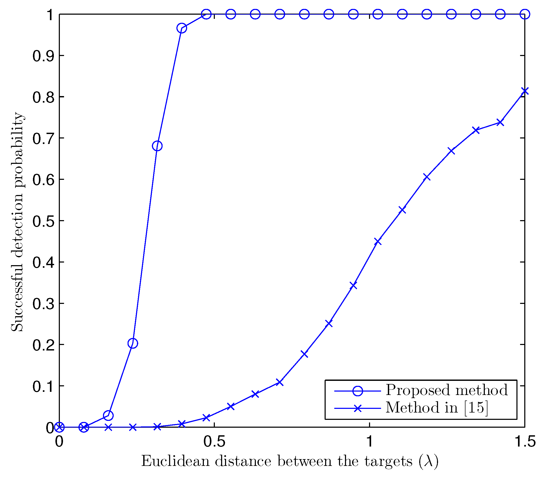
The resolution capability of a method can be evaluated by the probability of the successful detection of two closely-placed targets, which can be calculated as [12]:
where and is the half of the distance between the two targets. Figure 4 gives the probability of successful detection of two targets at different distances between the targets, which shows that the proposed method has a much better resolution power than its counterpart, even at the high signal-to-noise ratio (SNR) of 10 dB.
6. Discussion
In Figure 3, we can observe a significant gap between the RMSE corresponding to the proposed method and the method in [15]. The gain in performance of the proposed method comes from the use of the PARAFAC decomposition and the exact model of the received near-field signals. At high SNR, the method in [15] experiences a floor effect in terms of achievable RMSE performance, which clearly shows the systematic bias introduced by the approximated model. This systematic error is not discernible at low SNR because the major contribution to the estimation error comes from the noise. This bias also explains the low successful detection probability of [15], as shown in Figure 4. Because of the approximation, the location estimated by an approximated model-based method is shifted from the true location, which makes small.
7. Conclusions
In this paper, we propose a novel technique for near-field sources localization with a bistatic MIMO system. The principal originalities of this work are the use of the exact model and PARAFAC decomposition for near-field sources localization. Thanks to the exact model of near-field sources, the proposed method has high precision and resolution. The performance of the proposed method greatly surpasses the high-resolution subspace-based method proposed in [15], which proves the importance of an exact model-based method. The proposed method also has some additional advantages with respect to the compared approximated model-based method: it works for the inter-element spacing of without any ambiguity, M and N are not required to be odd, and any antenna can be used as the reference point.
Author Contributions
P.R.S., Y.W. and P.C. conceived and designed the proposed method; P.R.S. performed the development and programming; Y.W. and P.C. supervised the study; IETR contributed analysis tools; P.R.S., Y.W. and P.C. wrote the paper.
Conflicts of Interest
The authors declare no conflict of interest.
Abbreviations
The following abbreviations are used in this manuscript:
| CRLB | Cramér–Rao Lower Bound |
| ESPRIT | Estimation of Signal Parameter via Rotational Invariance Techniques |
| MIMO | Multiple Input Multiple Output |
| MUSIC | Multiple Signal Classification |
| PARAFAC | Parallel Factor |
| RMSE | Root Mean Square Error |
| SNR | Signal-to-Noise Ratio |
| TALS | Trilinear Alternating Least Squares |
| ULA | Uniform Linear Array |
References
- Van Trees, H.L. Optimum Array Processing: Part IV of Detection, Estimation, and Modulation Theory; John Wiley & Sons: Hoboken, NJ, USA, 2004. [Google Scholar]
- Li, J.; Stoica, P. MIMO Radar with Colocated Antennas. IEEE Signal Process. Mag. 2007, 24, 106–114. [Google Scholar] [CrossRef]
- Haimovich, A.M.; Blum, R.S.; Cimini, L.J. MIMO Radar with Widely Separated Antennas. IEEE Signal Process. Mag. 2008, 25, 116–129. [Google Scholar] [CrossRef]
- Yan, H.; Li, J.; Liao, G. Multitarget identification and localization using bistatic MIMO radar systems. EURASIP J. Adv. Signal Process. 2007, 2008, 1–8. [Google Scholar]
- Nion, D.; Sidiropoulos, N.D. A PARAFAC-based technique for detection and localization of multiple targets in a MIMO radar system. In Proceedings of the IEEE International Conference on Acoustics, Speech and Signal Processing (ICASSP), Taipei, Taiwan, 19–24 April 2009; pp. 2077–2080. [Google Scholar]
- Swindlehurst, A.L.; Kailath, T. Passive direction-of-arrival and range estimation for near-field sources. In Proceedings of the Fourth Annual ASSP Workshop on Spectrum Estimation and Modeling, Minneapolis, MN, USA, 3–5 August 1988; pp. 123–128. [Google Scholar]
- Grosicki, E.; Abed-Meraim, K.; Hua, Y. A weighted linear prediction method for near-field source localization. IEEE Trans. Signal Process. 2005, 53, 3651–3660. [Google Scholar] [CrossRef]
- Zhi, W.; Chia, M.W. Near-field source localization via symmetric subarrays. IEEE Signal Process. Lett. 2007, 14, 409–412. [Google Scholar] [CrossRef]
- He, H.; Wang, Y.; Saillard, J. A high resolution method of source localization in near-field by using focusing technique. In Proceedings of the European Signal Processing Conference, Lausanne, Switzerland, 25–29 August 2008; pp. 1–5. [Google Scholar]
- Guo, Y.D.; Xie, H.; Zhang, Y.S.; Gong, J.; Shen, D. Localization for Near-Field Targets Based on Virtual Array of MIMO radar. Radar Sci. Technol. 2012, 10, 82–87. [Google Scholar]
- He, J.; Swamy, M.; Ahmad, M.O. Efficient application of MUSIC algorithm under the coexistence of far-field and near-field sources. IEEE Trans. Signal Process. 2012, 60, 2066–2070. [Google Scholar] [CrossRef]
- Wang, B.; Zhao, Y.; Liu, J. Mixed-order MUSIC algorithm for localization of far-field and near-field sources. IEEE Signal Process. Lett. 2013, 20, 311–314. [Google Scholar] [CrossRef]
- Begriche, Y.; Thameri, M.; Abed-Meraim, K. Exact conditional and unconditional Cramér–Rao bounds for near field localization. Digit. Signal Process. 2014, 31, 45–58. [Google Scholar] [CrossRef]
- Li, J.; Wang, Y.; Gang, W. Signal reconstruction for near-field source localisation. IET Signal Process. 2015, 9, 201–205. [Google Scholar]
- Zhou, E.; Jiang, H.; Qi, H. 4-D parameter estimation in bistatic MIMO radar for near-field target localization. In Proceedings of the International Wireless Symposium (IWS), IEEE, Shenzhen, China, 30 March–1 April 2015; pp. 1–4. [Google Scholar]
- Li, J.; Wang, Y.; Le Bastard, C.; Wei, G.; Ma, B.; Sun, M.; Yu, Z. Simplified High-order DOA and Range Estimation with Linear Antenna Array. IEEE Commun. Lett. 2017, 21, 76–79. [Google Scholar] [CrossRef]
- Singh, P.R.; Wang, Y.; Chargé, P. Bistatic MIMO radar for near field source localisation using PARAFAC. Electron. Lett. 2016, 52, 1060–1061. [Google Scholar] [CrossRef]
- Nion, D.; Sidiropoulos, N.D. Tensor algebra and multidimensional harmonic retrieval in signal processing for MIMO radar. IEEE Trans. Signal Process. 2010, 58, 5693–5705. [Google Scholar] [CrossRef]
- Kruskal, J.B. Three-way arrays: Rank and uniqueness of trilinear decompositions, with application to arithmetic complexity and statistics. Linear Algebra Its Appl. 1977, 18, 95–138. [Google Scholar] [CrossRef]
- Cichocki, A.; Mandic, D.P.; Phan, A.H.; Caiafa, C.F.; Zhou, G.; Zhao, Q.; De Lathauwer, L. Tensor decompositions for signal processing applications: From two-way to multiway component analysis. IEEE Signal Process. Mag. 2015, 32, 145–163. [Google Scholar] [CrossRef]
- Swerling, P. Probability of detection for fluctuating targets. IRE Trans. Inf. Theory 1960, 6, 269–308. [Google Scholar] [CrossRef]
- Harshman, R.A. Foundations of the PARAFAC Procedure: Models and Conditions for an “Explanatory“ Multimodal Factor Analysis; Working Papers in Phonetics (WPP); Department of Linguistics, University of California at Los Angeles (UCLA), University Microfilms: Ann Arbor, MI, USA, 1970; Volume 16, pp. 1–84. [Google Scholar]
- Carroll, J.D.; Chang, J.J. Analysis of individual differences in multidimensional scaling via an N-way generalization of “Eckart-Young” decomposition. Psychometrika 1970, 35, 283–319. [Google Scholar] [CrossRef]
- Bro, R.; Sidiropoulos, N.D.; Giannakis, G.B. A fast least squares algorithm for separating trilinear mixtures. In Proceedings of the International Workshop on Independent Component Analysis and Blind Separation, Aussois, France, 11–15 January 1999; pp. 11–15. [Google Scholar]
- Tribolet, J. A new phase unwrapping algorithm. IEEE Trans. Acoust. Speech Signal Process. 1977, 25, 170–177. [Google Scholar] [CrossRef]
- Golub, G.H.; Loan, C.V. Total least squares. In Smoothing Techniques for Curve Estimation; Springer: Heidelberg, Germany, 1979; pp. 69–76. [Google Scholar]
- Stoica, P.; Larsson, E.G.; Gershman, A.B. The Stochastic CRB for Array Processing: A Textbook Derivation. IEEE Signal Process. Lett. 2001, 8, 148–150. [Google Scholar] [CrossRef]
Figure 1.
Tensorization.

Figure 2.
General configuration of a bistatic multiple input, multiple output (MIMO) radar system with linear arrays.
Figure 2.
General configuration of a bistatic multiple input, multiple output (MIMO) radar system with linear arrays.
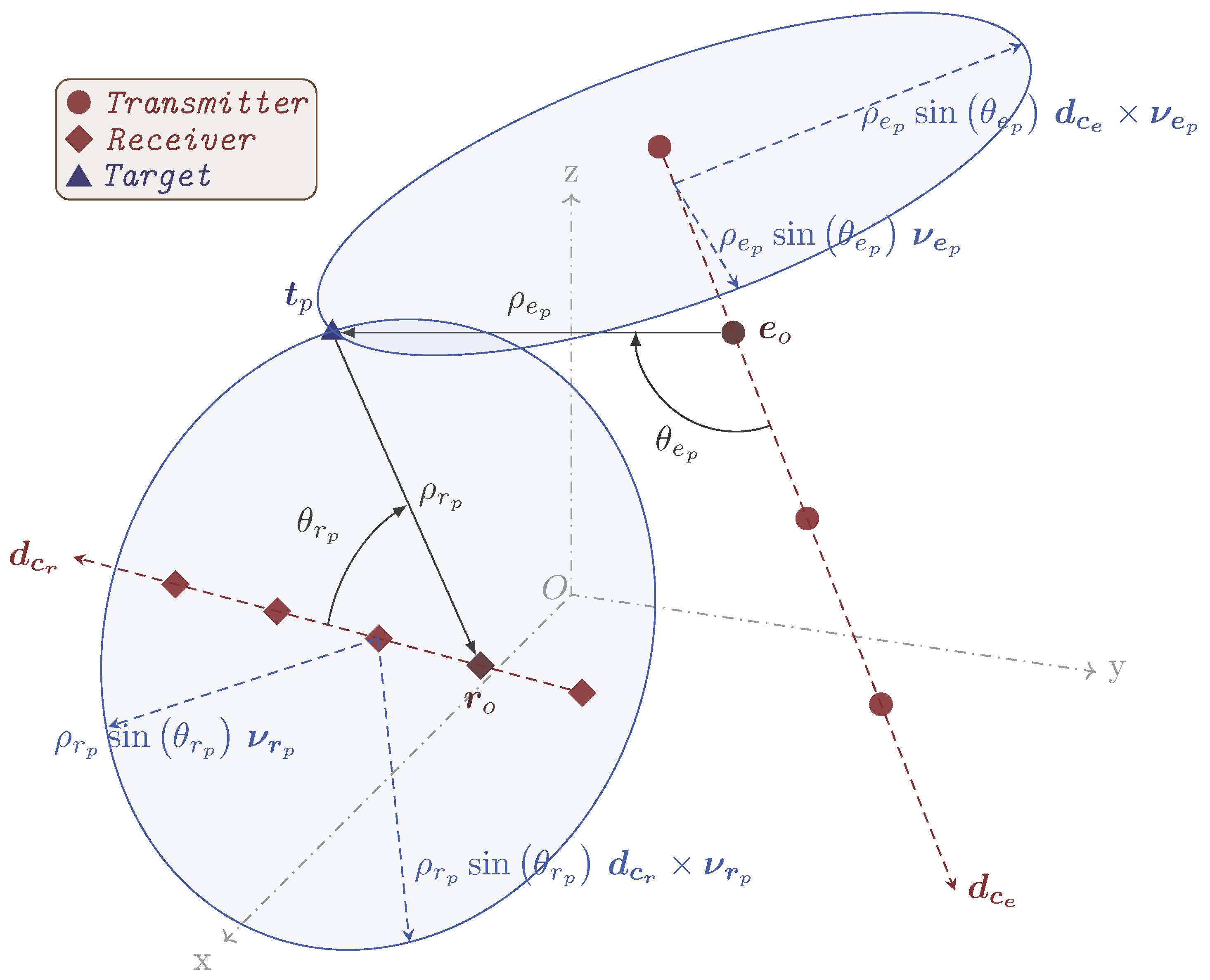
Figure 3.
Root mean square error (RMSE) versus signal-to-noise ratio (SNR); , , , , , and . CRLB: Cramér–Rao lower bound.
Figure 3.
Root mean square error (RMSE) versus signal-to-noise ratio (SNR); , , , , , and . CRLB: Cramér–Rao lower bound.

Figure 4.
Probability of successful detection versus distance between two targets at SNR dB; , , , , , and .
Figure 4.
Probability of successful detection versus distance between two targets at SNR dB; , , , , , and .
© 2017 by the authors. Licensee MDPI, Basel, Switzerland. This article is an open access article distributed under the terms and conditions of the Creative Commons Attribution (CC BY) license (http://creativecommons.org/licenses/by/4.0/).
Share and Cite
MDPI and ACS Style
Singh, P.R.; Wang, Y.; Chargé, P. An Exact Model-Based Method for Near-Field Sources Localization with Bistatic MIMO System. Sensors 2017, 17, 723. https://doi.org/10.3390/s17040723
AMA Style
Singh PR, Wang Y, Chargé P. An Exact Model-Based Method for Near-Field Sources Localization with Bistatic MIMO System. Sensors. 2017; 17(4):723. https://doi.org/10.3390/s17040723
Chicago/Turabian StyleSingh, Parth Raj, Yide Wang, and Pascal Chargé. 2017. "An Exact Model-Based Method for Near-Field Sources Localization with Bistatic MIMO System" Sensors 17, no. 4: 723. https://doi.org/10.3390/s17040723
Note that from the first issue of 2016, this journal uses article numbers instead of page numbers. See further details here.