
Smooth Sensor Motion Planning for Robotic Cyber Physical Social Sensing (CPSS)


Abstract
:1. Introduction
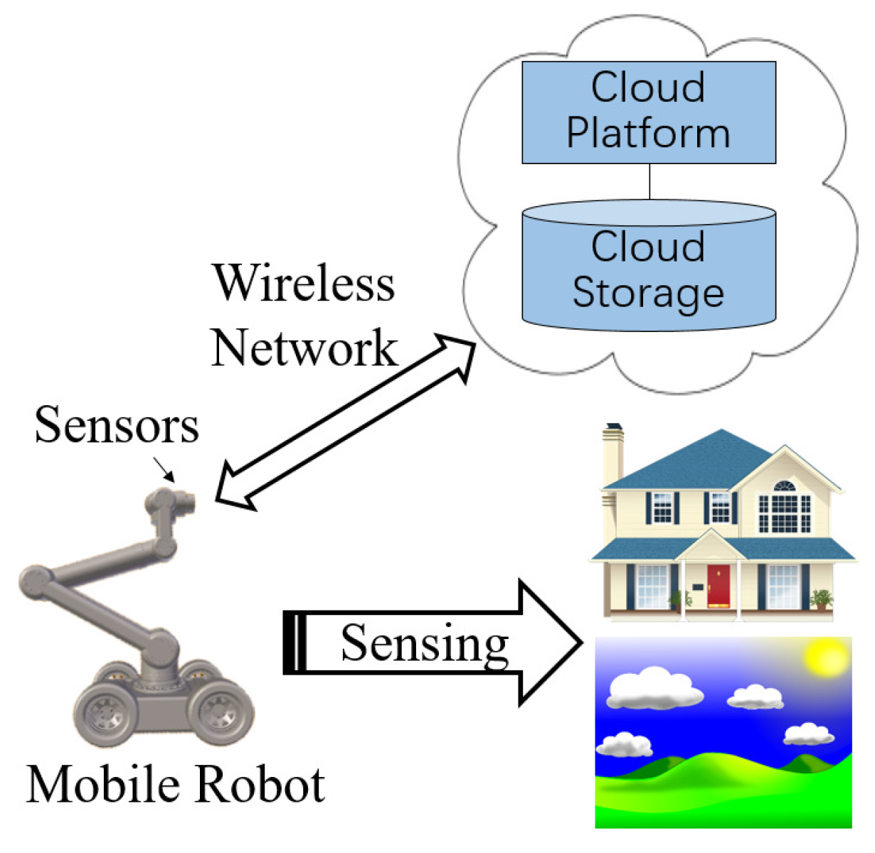
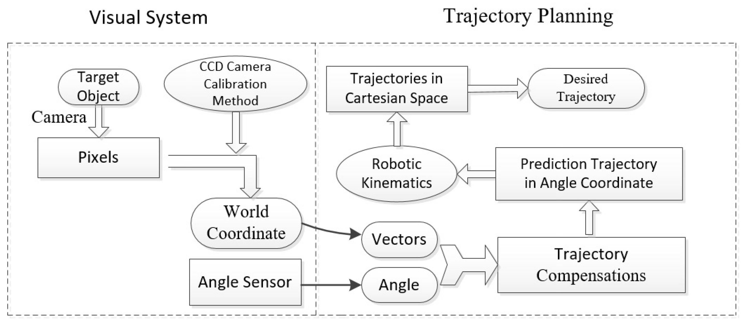
2. System Overview
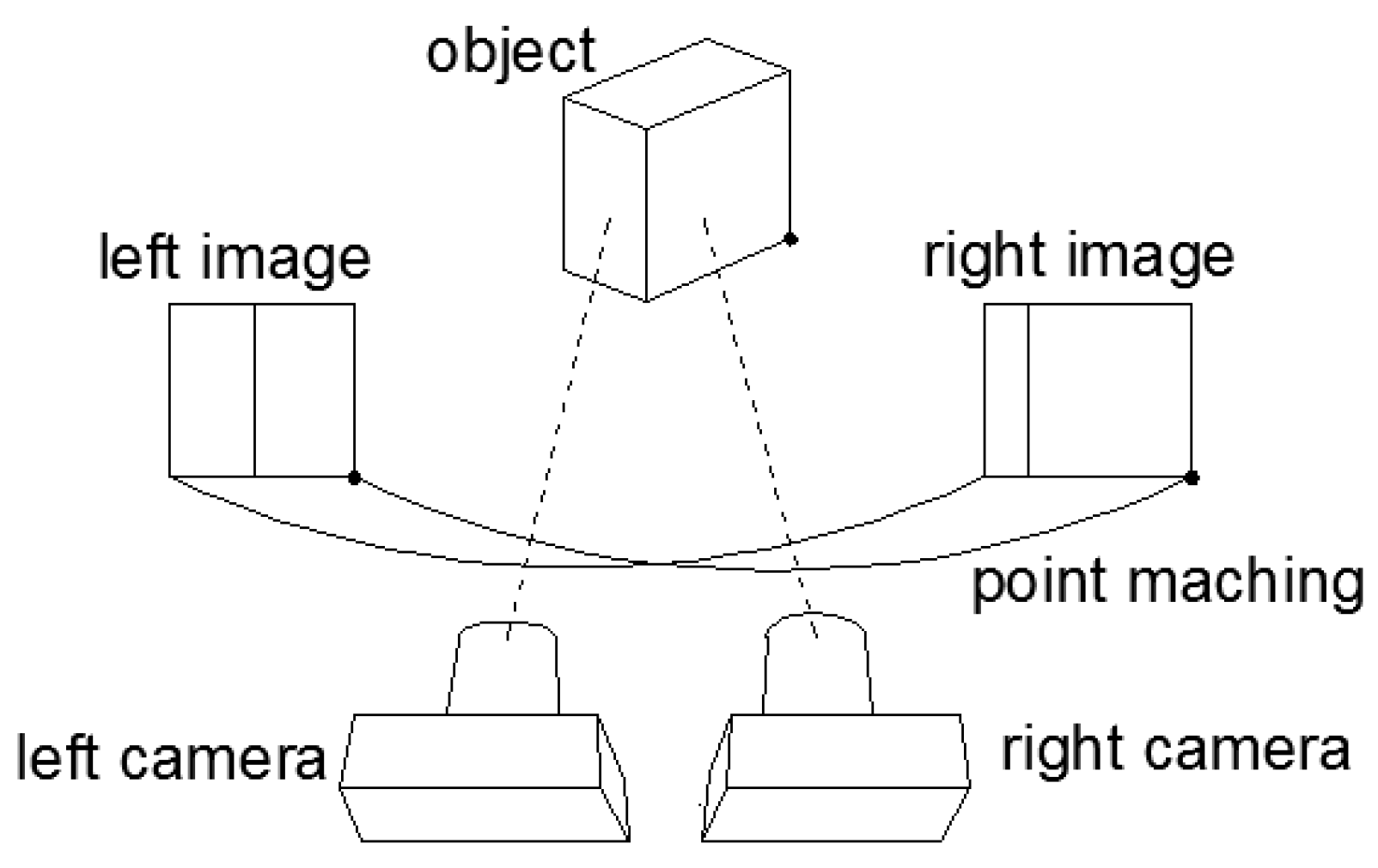
2.1. Binocular Vision Sensor
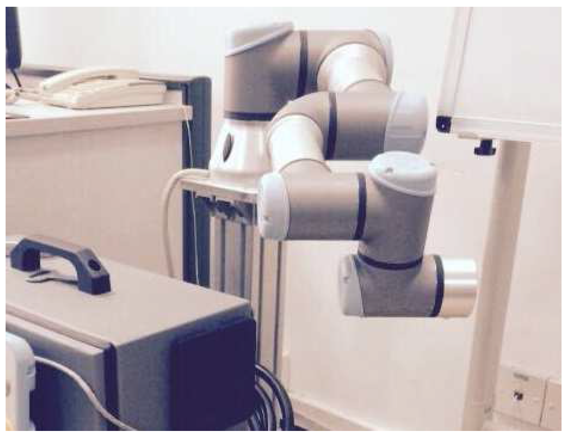
2.2. Testing Platform
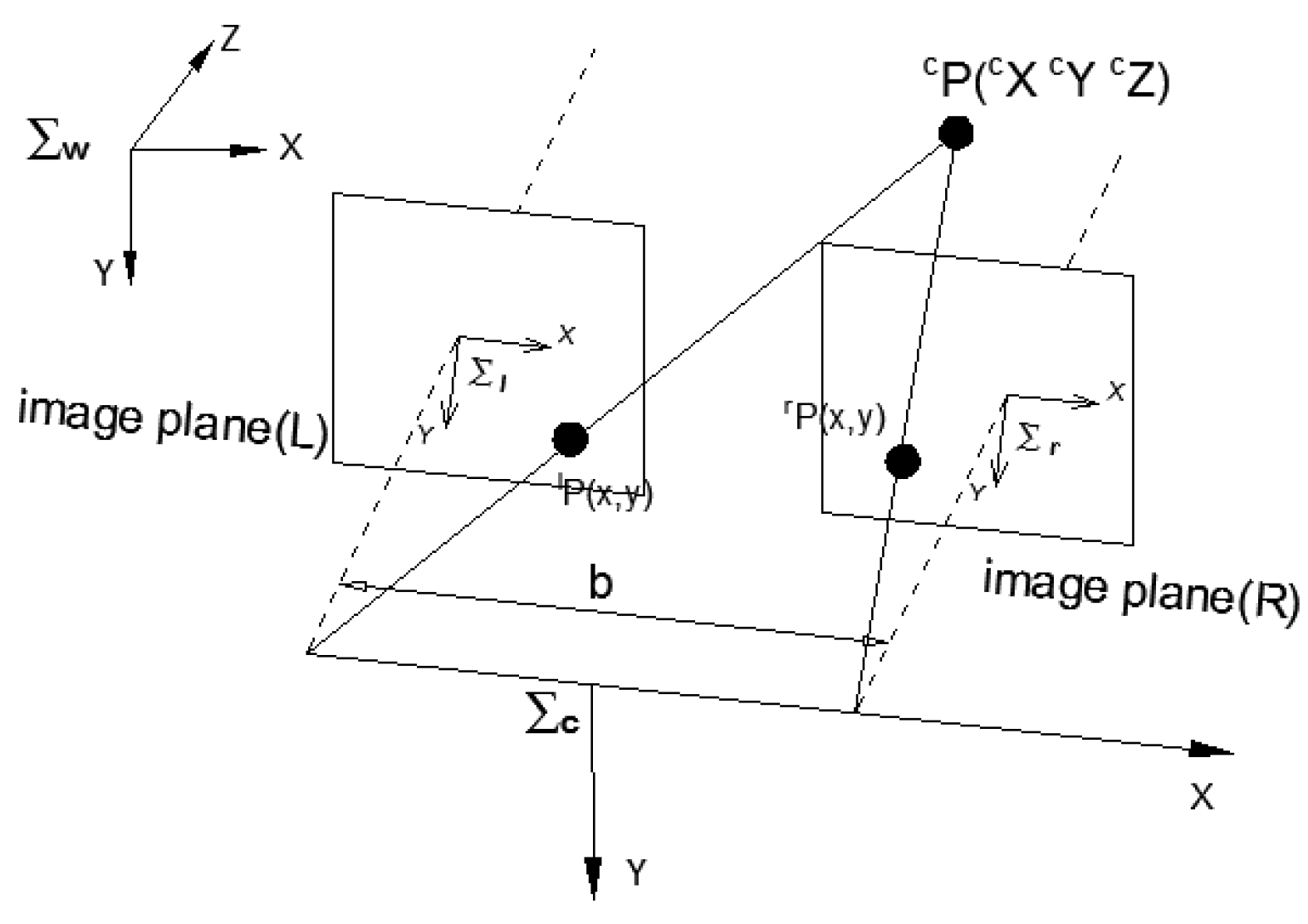
3. Binocular Stereo Vision Sensor System
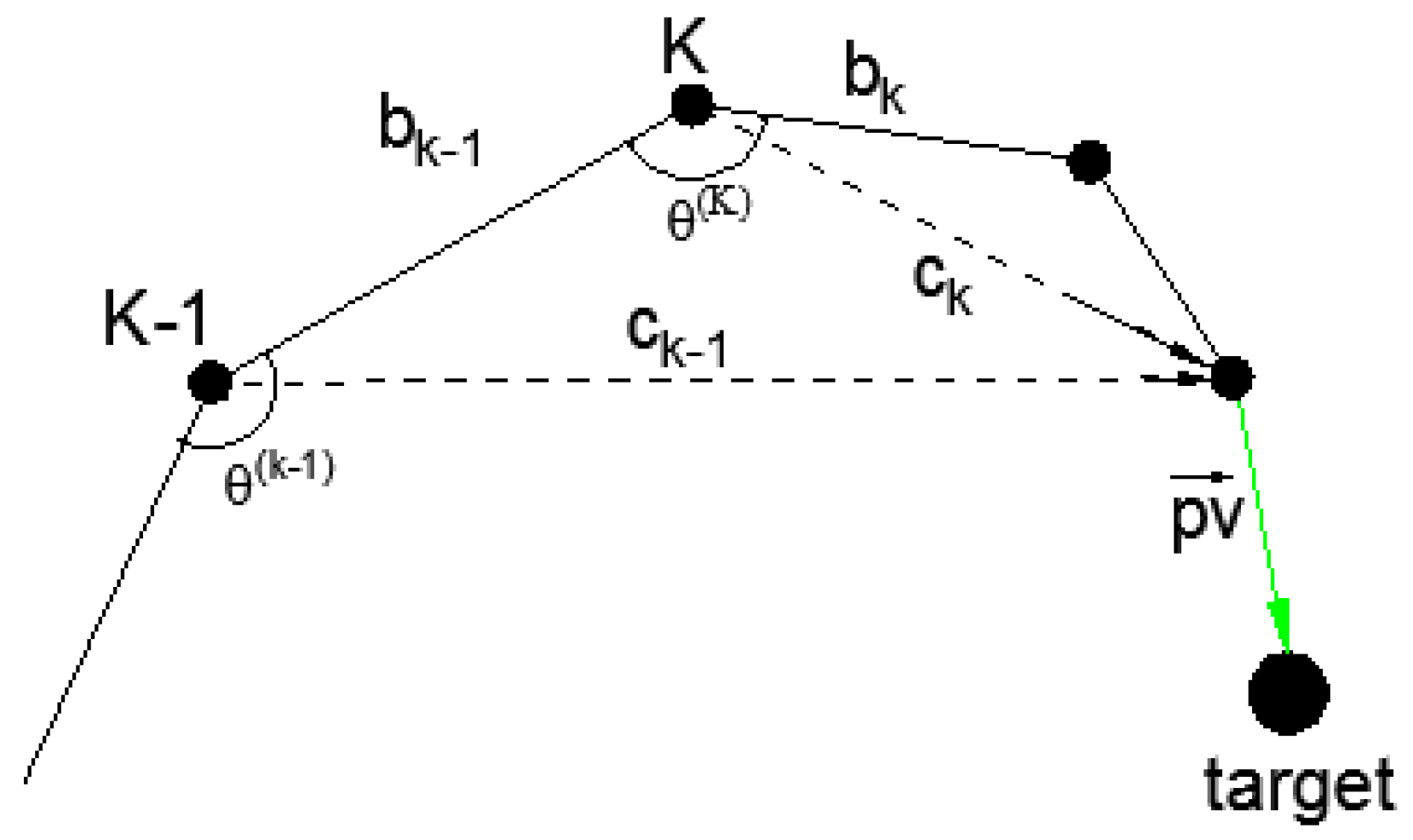
4. Trajectory Planning For Binocular Stereo Sensors
4.1. Joint Space-Based Trajectory Planning
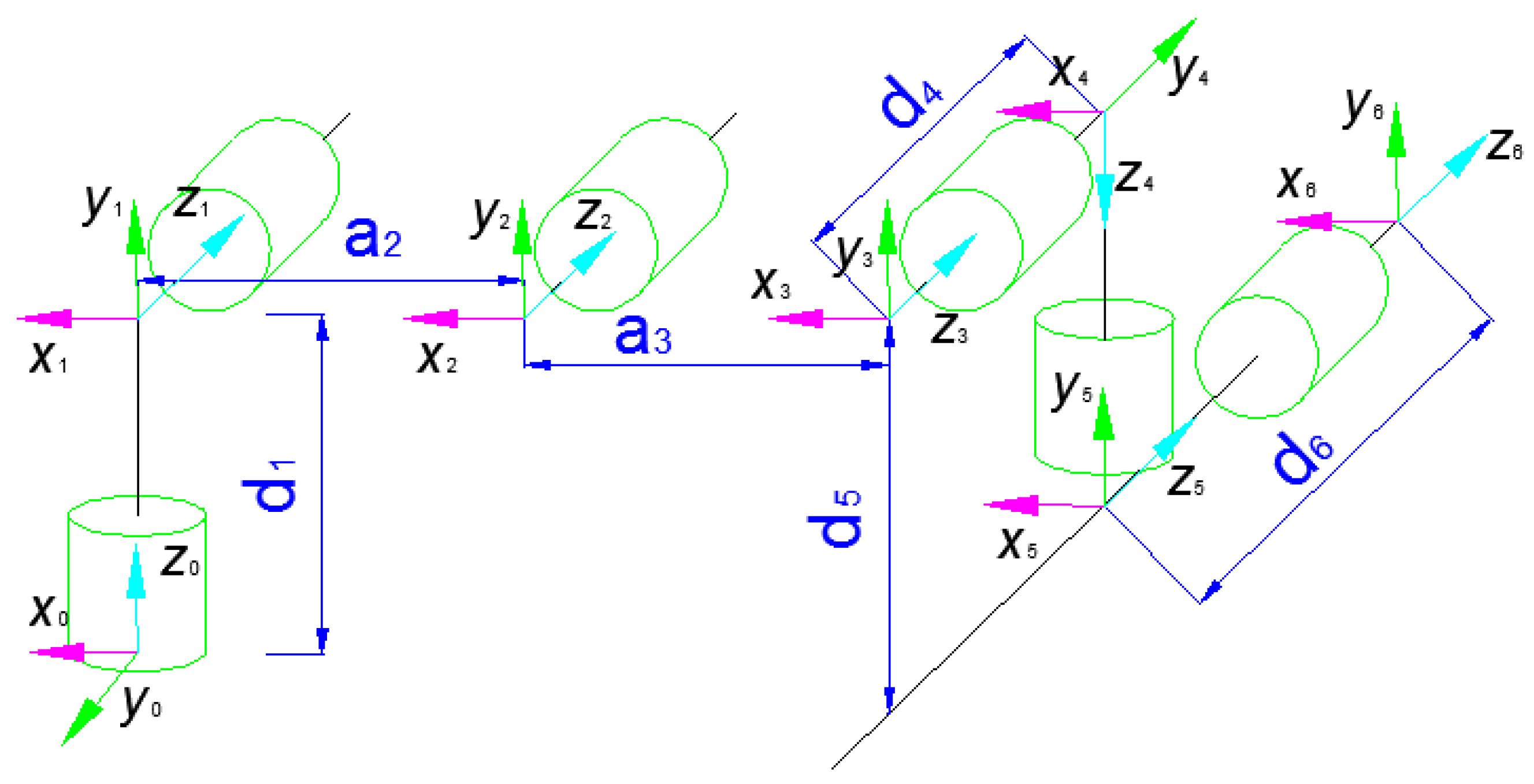
4.2. Coordinate Transformation
4.3. Joint State
| Algorithm 1: Trajectory Planning |
 |
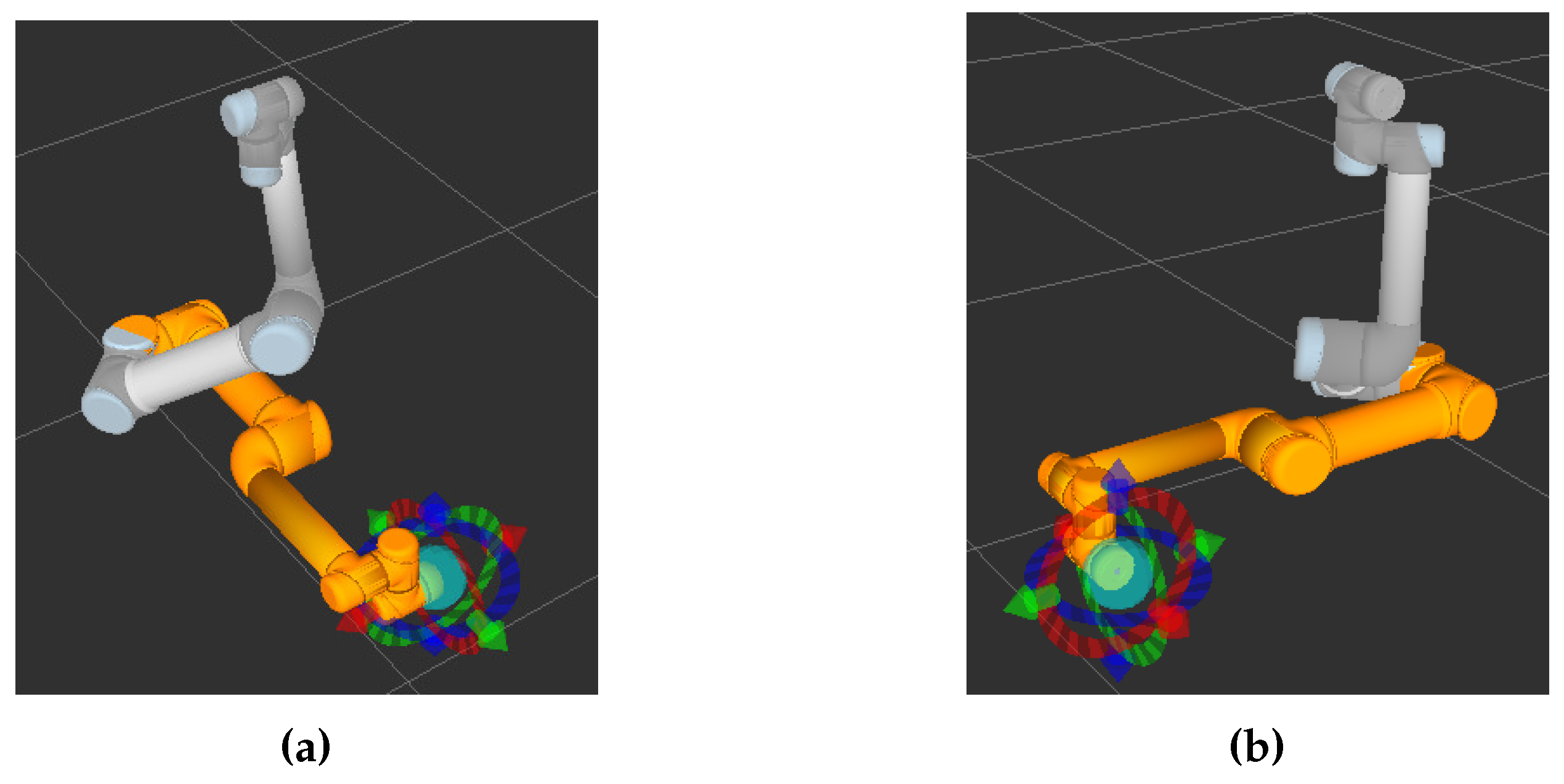
5. Experiments and Analysis
5.1. Experiment Environment
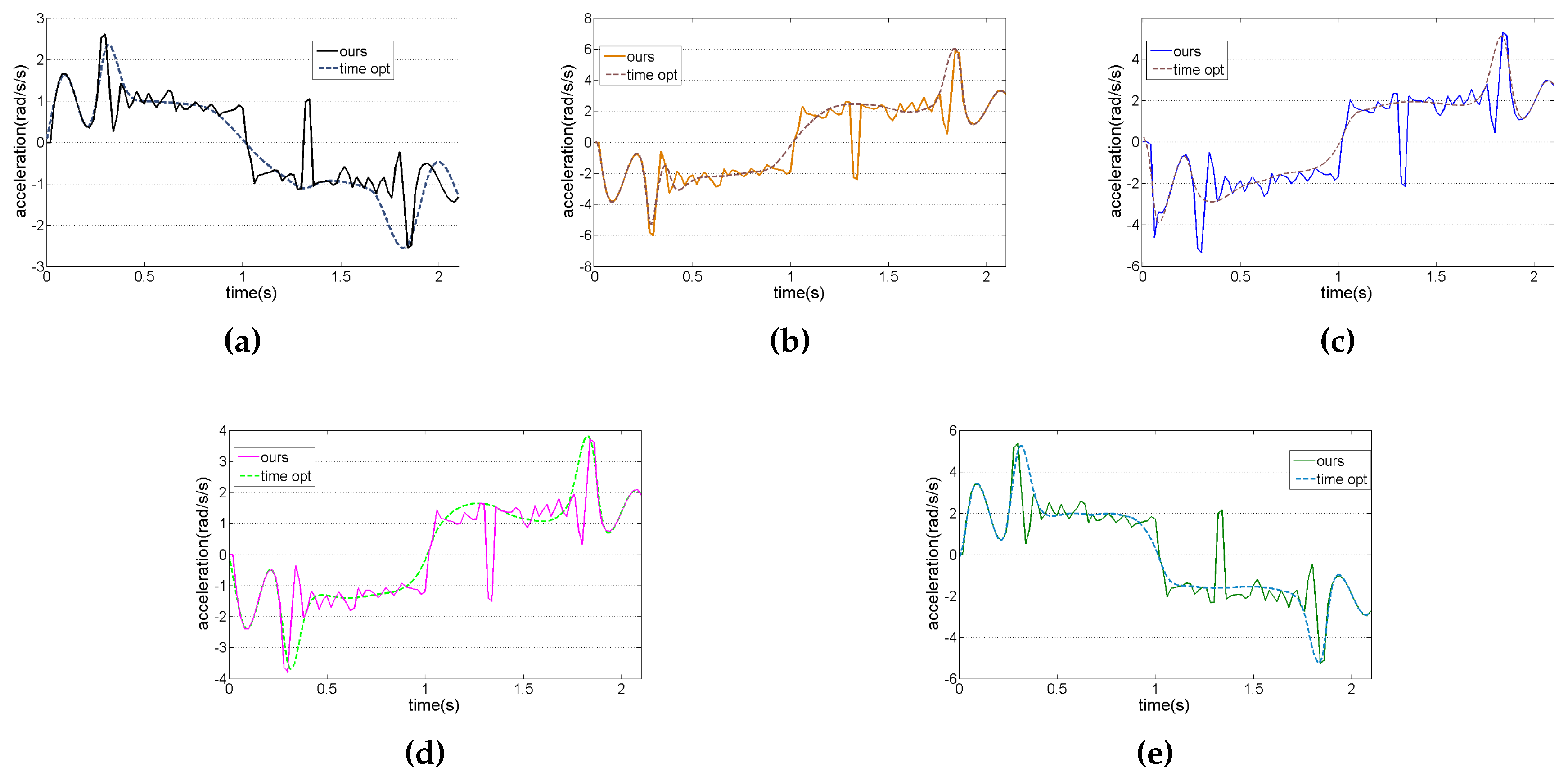
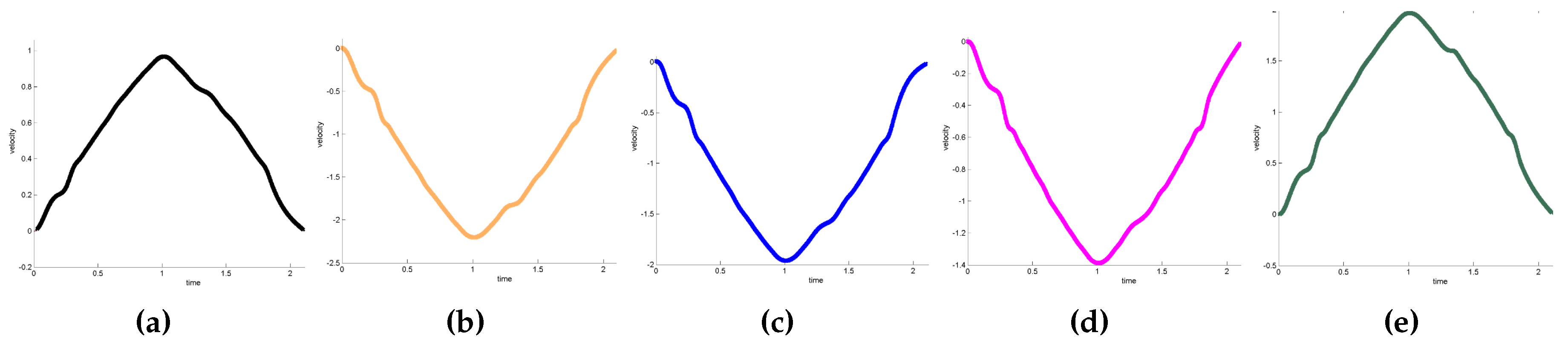
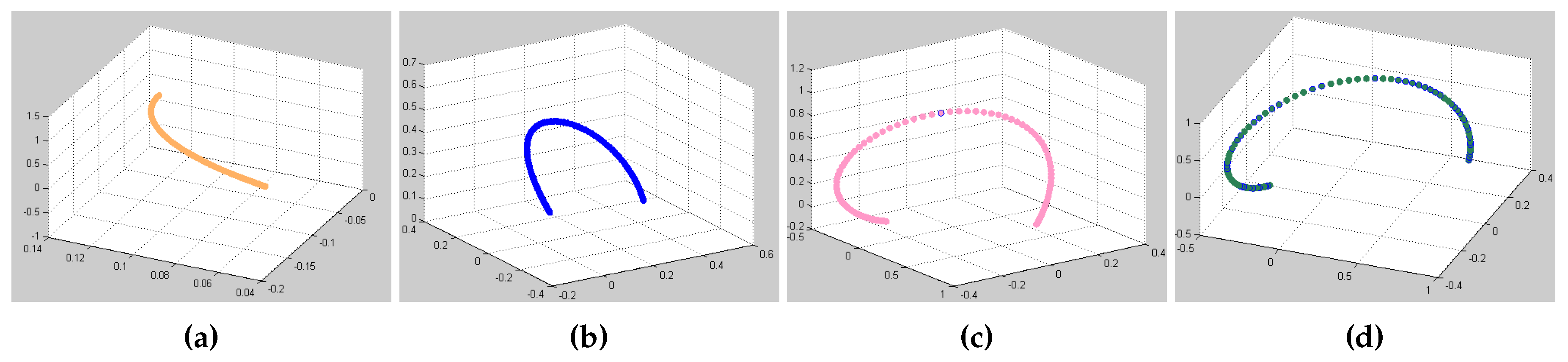
5.2. Experimental Results
6. Conclusions
Acknowledgments
Author Contributions
Conflicts of Interest
References
- Dong, M.; Ota, K.; Liu, A. RMER: Reliable and Energy-Efficient Data Collection for Large-Scale Wireless Sensor Networks. IEEE Internet Things J. 2016, 3, 511–519. [Google Scholar] [CrossRef]
- Liu, Y.; Dong, M.; Ota, K.; Liu, A. ActiveTrust: Secure and Trustable Routing in Wireless Sensor Networks. IEEE Trans. Inf. For. Secur. 2016, 11, 2013–2027. [Google Scholar] [CrossRef]
- Dong, M.; Ota, K.; Yang, L.T.; Liu, A.; Guo, M. LSCD: A Low-Storage Clone Detection Protocol for Cyber-Physical Systems. IEEE Trans. Comput.-Aided Des. Integr. Circuits Syst. 2016, 35, 712–723. [Google Scholar] [CrossRef]
- Liu, X.; Dong, M.; Ota, K.; Hung, P.; Liu, A. Service Pricing Decision in Cyber-Physical Systems: Insights from Game Theory. IEEE Trans. Serv. Comput. 2016, 9, 186–198. [Google Scholar] [CrossRef]
- Korayem, M.; Nikoobin, A. Maximum payload for flexible joint manipulators in point-to-point task using optimal control approach. Int. J. Adv. Manuf. Technol. 2008, 38, 1045–1060. [Google Scholar] [CrossRef]
- Menasri, R.; Oulhadj, H.; Daachi, B.; Nakib, A.; Siarry, P. A genetic algorithm designed for robot trajectory planning. In Proceedings of the 2014 IEEE International Conference on Systems, Man, and Cybernetics (SMC), San Diego, CA, USA, 5–8 October 2014; pp. 228–233.
- Zefran, M.; Kumar, V.; Croke, C.B. On the generation of smooth three-dimensional rigid body motions. IEEE Trans. Robot. Autom. 1998, 14, 576–589. [Google Scholar] [CrossRef]
- Kröger, T.; Wahl, F.M. Online trajectory generation: Basic concepts for instantaneous reactions to unforeseen events. IEEE Trans. Robot. 2010, 26, 94–111. [Google Scholar] [CrossRef]
- Gasparetto, A.; Zanotto, V. A new method for smooth trajectory planning of robot manipulators. Mech. Mach. Theory 2007, 42, 455–471. [Google Scholar] [CrossRef]
- Piazzi, A.; Visioli, A. Global minimum-jerk trajectory planning of robot manipulators. IEEE Trans. Ind. Electron. 2000, 47, 140–149. [Google Scholar] [CrossRef]
- Kanade, T.; Okutomi, M. A stereo matching algorithm with an adaptive window: Theory and experiment. IEEE Trans. Pattern Anal. Mach. Intell. 1994, 16, 920–932. [Google Scholar] [CrossRef]
- Li, Z. Visual Servoing in Robotic Manufacturing Systems for Accurate Positioning. Ph.D. Thesis, Concordia University, Montreal, QC, Canada, 2007. [Google Scholar]
- Murray, R.M.; Li, Z.; Sastry, S.S.; Sastry, S.S. A Mathematical Introduction to Robotic Manipulation; CRC Press: Boca Raton, FL, USA, 1994. [Google Scholar]
- Nan-feng, X. Intelligent Robot; South China University of Technology Press: Guangzhou, China, 2008; pp. 104–105. [Google Scholar]
- Craig, J.J. Introduction to Robotics: Mechanics and Control; Pearson Prentice Hall: Upper Saddle River, NJ, USA, 2005; Volume 3. [Google Scholar]
- Marani, G.; Kim, J.; Yuh, J.; Chung, W.K. A real-time approach for singularity avoidance in resolved motion rate control of robotic manipulators. In Proceedings of the ICRA’02 IEEE International Conference on Robotics and Automation, Atlanta, GA, USA, 11–15 May 2002; Volume 2, pp. 1973–1978.
- Zorjan, M.; Hugel, V. Generalized humanoid leg inverse kinematics to deal with singularities. In Proceedings of the 2013 IEEE International Conference on Robotics and Automation (ICRA), Karlsruhe, Germany, 6–10 May 2013; pp. 4791–4796.
- Li, L.; Xiao, N. Volumetric view planning for 3D reconstruction with multiple manipulators. Ind. Robot Int. J. 2015, 42, 533–543. [Google Scholar] [CrossRef]
- Dutta, T. Evaluation of the Kinect™ sensor for 3-D kinematic measurement in the workplace. Appl. Ergon. 2012, 43, 645–649. [Google Scholar] [CrossRef] [PubMed]
- Zhang, Z. Flexible camera calibration by viewing a plane from unknown orientations. In Proceedings of the Seventh IEEE International Conference on Computer Vision, Kerkyra, Greece, 20–27 September 1999; Volume 1, pp. 666–673.
- Liu, H.; Lai, X.; Wu, W. Time-optimal and jerk-continuous trajectory planning for robot manipulators with kinematic constraints. Robot. Comput. Integr. Manuf. 2013, 29, 309–317. [Google Scholar] [CrossRef]


| Joints | 1 | 2 | 3 | 4 | 5 | 6 |
|---|---|---|---|---|---|---|
| Torsion angle (rad) | 0 | 0 | 0 | |||
| Rod length (mm) | 0 | –425 | –392 | 0 | 0 | 0 |
| Bias length (mm) | 89.2 | 0 | 0 | 109.3 | 94.75 | 82.5 |
| Joint angle | ||||||
| Constraint of joint (rad) |
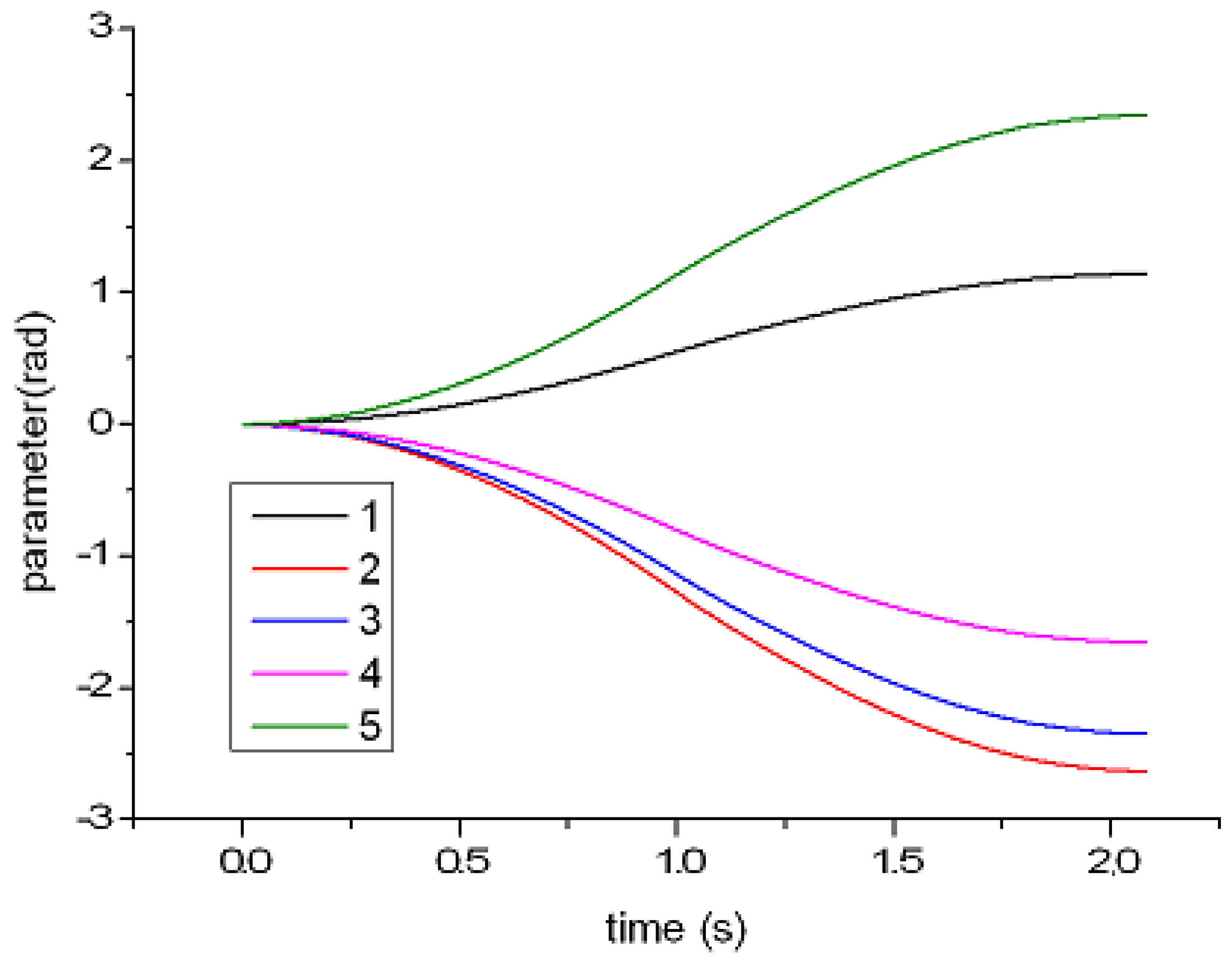
| θ | Initial State | Terminate State |
|---|---|---|
| 1 | 0 | 1.142958 |
| 2 | 0 | –2.630475 |
| 3 | 0 | –2.346571 |
| 4 | 0 | –1.654041 |
| 5 | 0 | 2.346625 |
| 6 | 0 | 0 |
| No. | Coordinates of Target | Final Position Coordinate (Time-Optimal/Ours) | Absolute Errors (Time-Optimal/Ours) |
|---|---|---|---|
| 1 | (328.04,115.59,341.21) | (336.34,124.31,351.14); (329.73,117.62,342.67) | 15.63; 3.02 |
| 2 | (349.76,273.16,345.68) | (354.13,274.89,349.98); (361.22,275.72,346.12) | 6.68; 2.97 |
| 3 | (401.58,178.29,323.17) | (407.19,183.62,324.55); (401.77,180.37,323.98) | 7.87; 2.24 |
| 4 | (345.43,242.75,350.48) | (352.04,247.70,356.78); (345.54,244.85,352.44) | 10.39; 2.87 |
| 5 | (327.12,–41.74,301.31) | (332.79,–34.30,303.20); (328.80,–41.57,301.83) | 9.54; 1.77 |
© 2017 by the authors. Licensee MDPI, Basel, Switzerland. This article is an open access article distributed under the terms and conditions of the Creative Commons Attribution (CC BY) license ( http://creativecommons.org/licenses/by/4.0/).
Share and Cite
Tang, H.; Li, L.; Xiao, N. Smooth Sensor Motion Planning for Robotic Cyber Physical Social Sensing (CPSS). Sensors 2017, 17, 393. https://doi.org/10.3390/s17020393
Tang H, Li L, Xiao N. Smooth Sensor Motion Planning for Robotic Cyber Physical Social Sensing (CPSS). Sensors. 2017; 17(2):393. https://doi.org/10.3390/s17020393
Chicago/Turabian StyleTang, Hong, Liangzhi Li, and Nanfeng Xiao. 2017. "Smooth Sensor Motion Planning for Robotic Cyber Physical Social Sensing (CPSS)" Sensors 17, no. 2: 393. https://doi.org/10.3390/s17020393