
Evaluation of the Vegetation Coverage Resilience in Areas Damaged by the Wenchuan Earthquake Based on MODIS-EVI Data


Abstract
:
1. Introduction
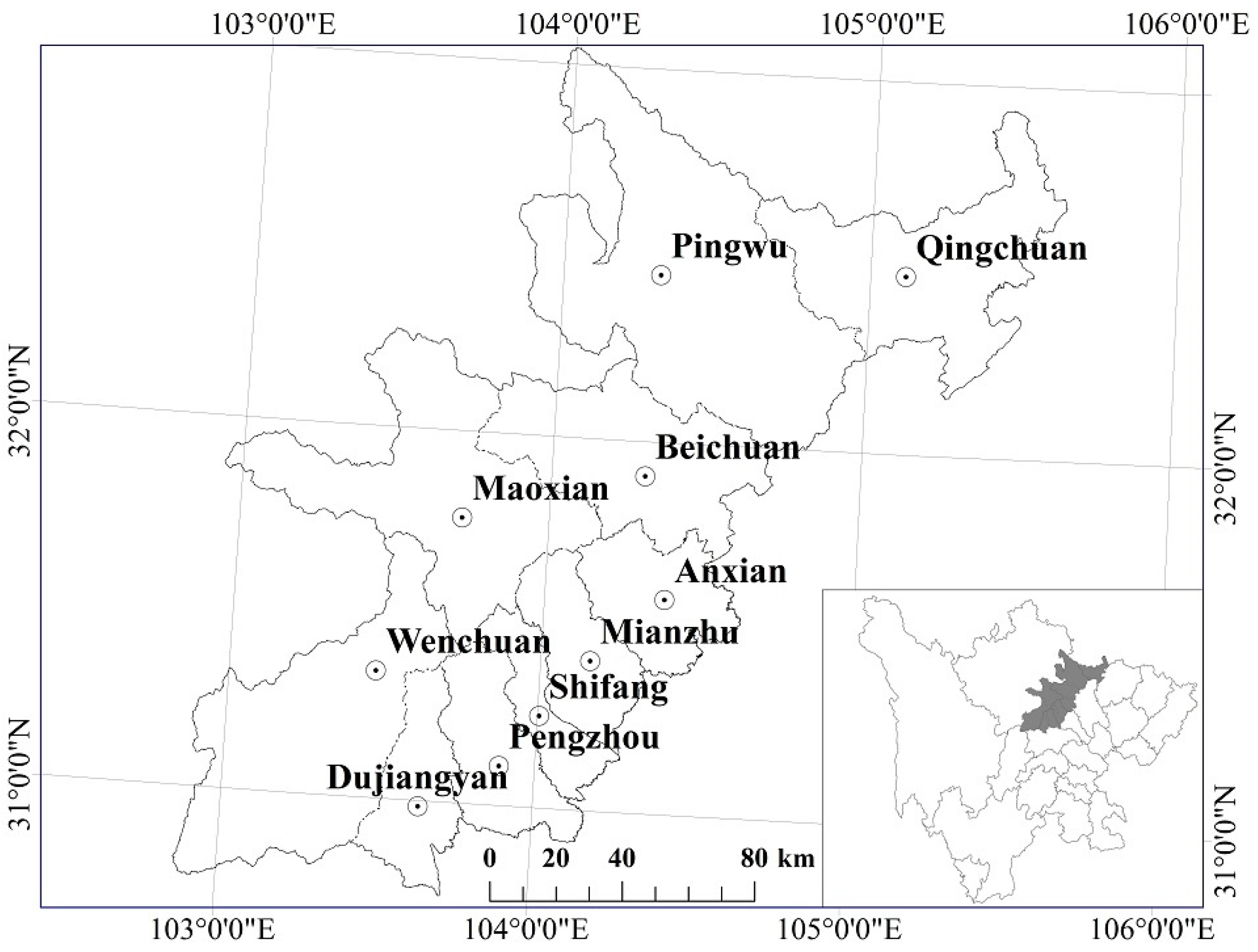
2. Study Area
3. Data Source
4. Methods
4.1. The Maximum Value Composite
4.2. Identification of the Damaged Area
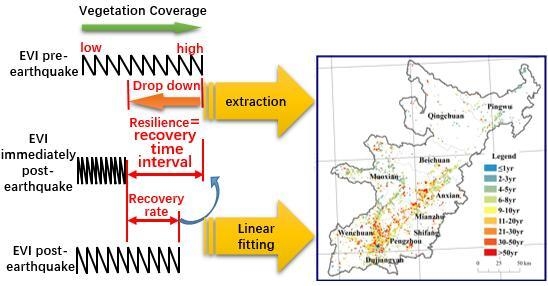
4.3. Definition and Measurement of Resilience
5. Results
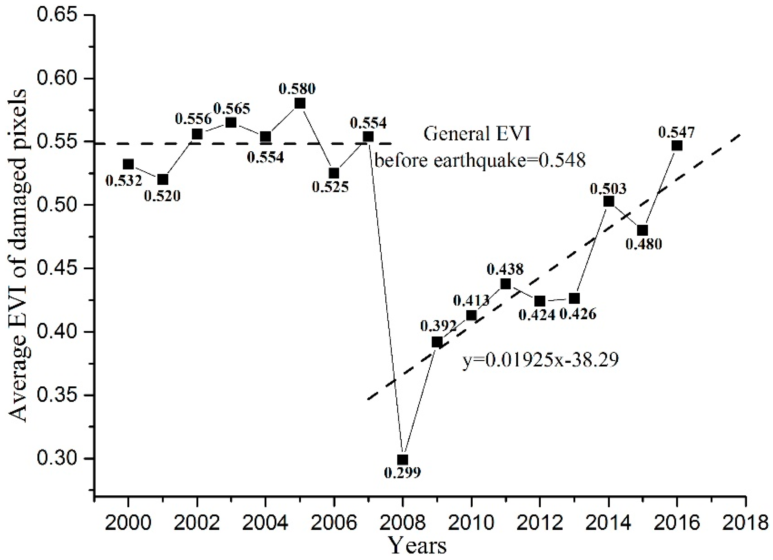
5.1. Dynamics of the Vegetation Coverage in the Damaged Areas
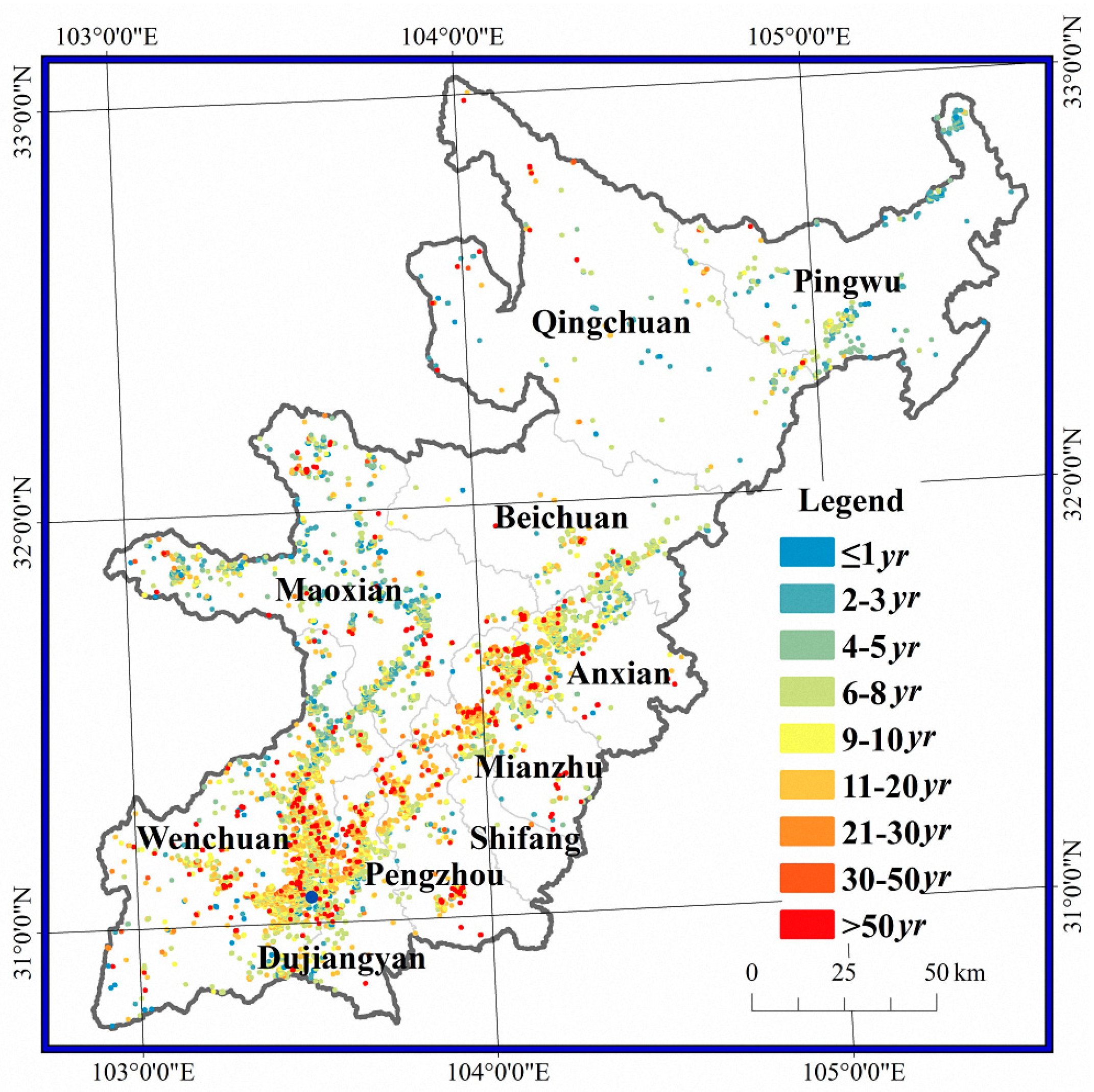
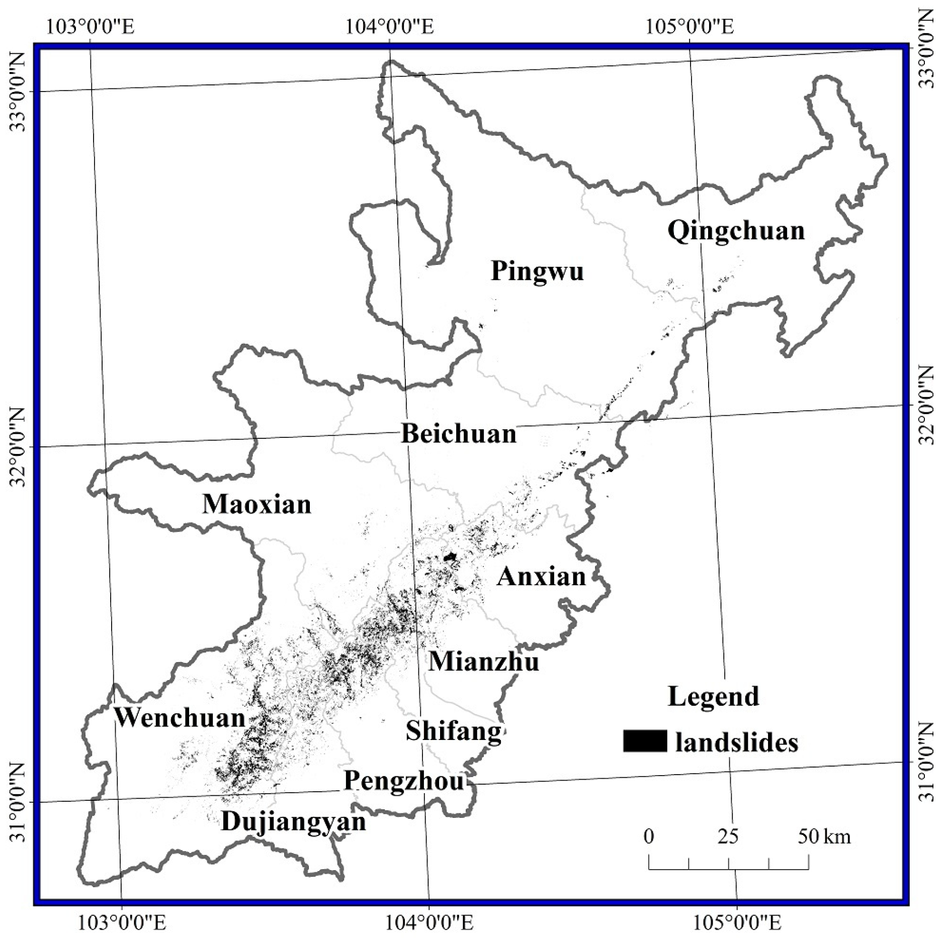
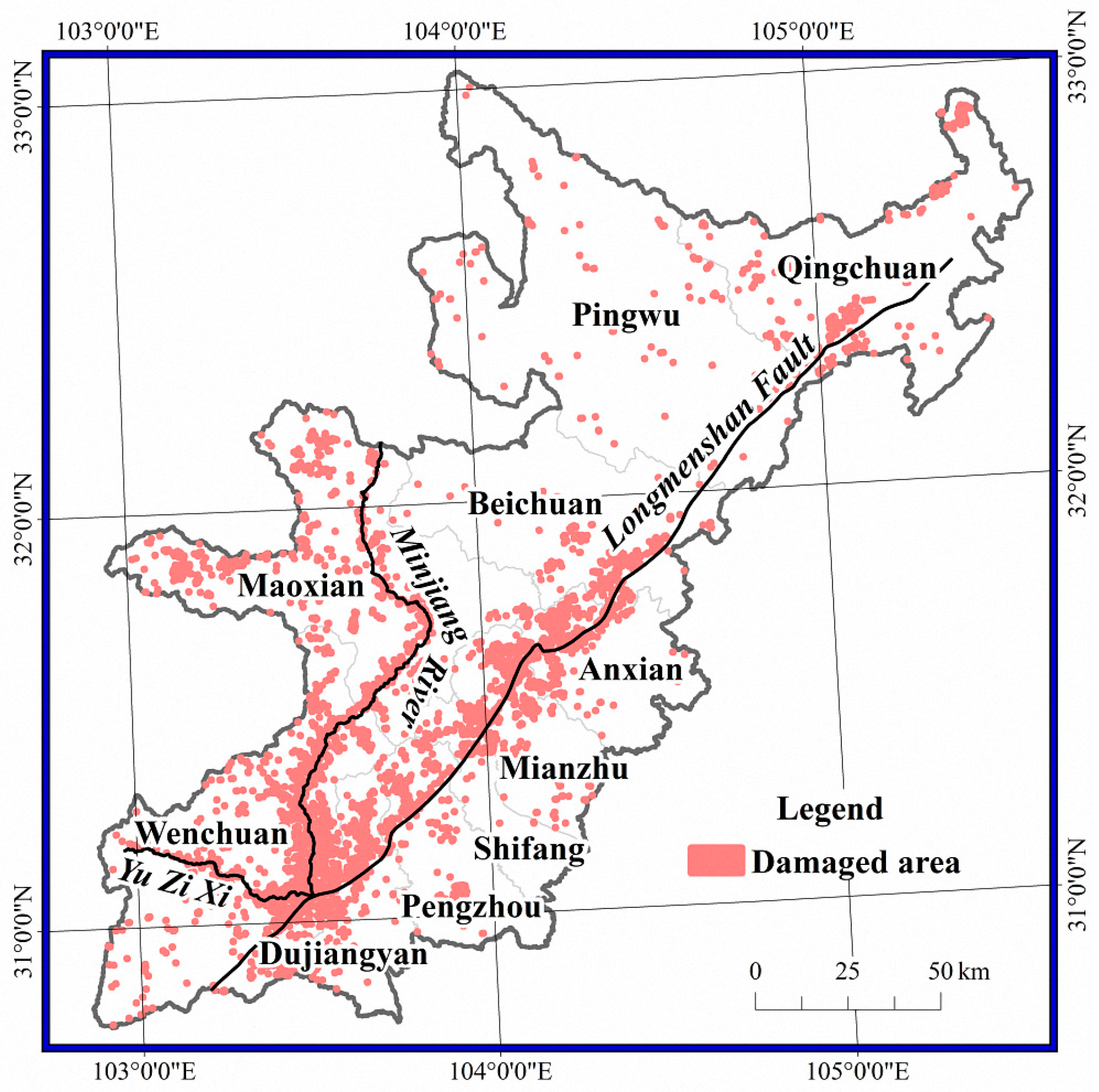
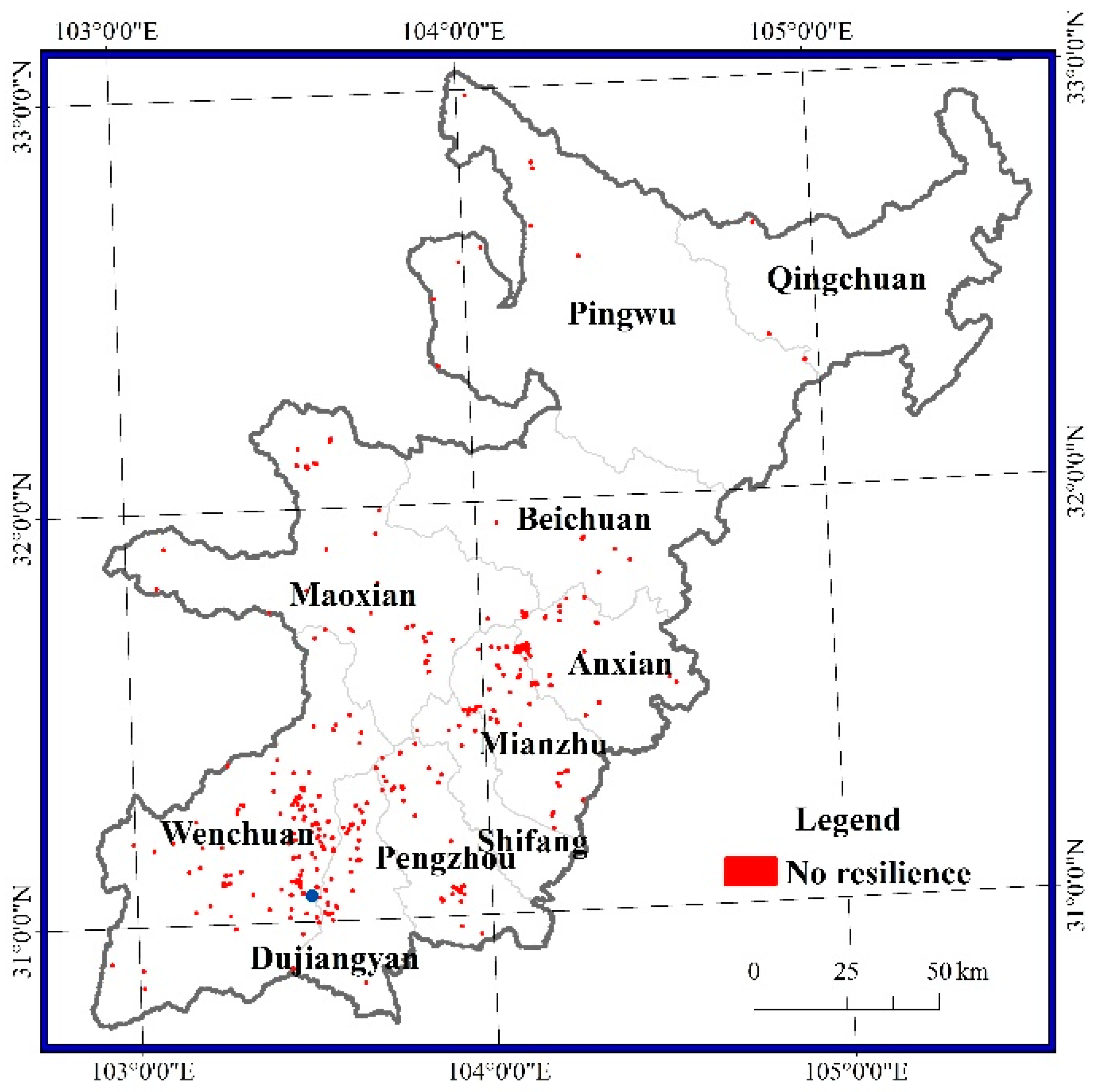
5.2. Spatial Distribution of the Damaged Areas
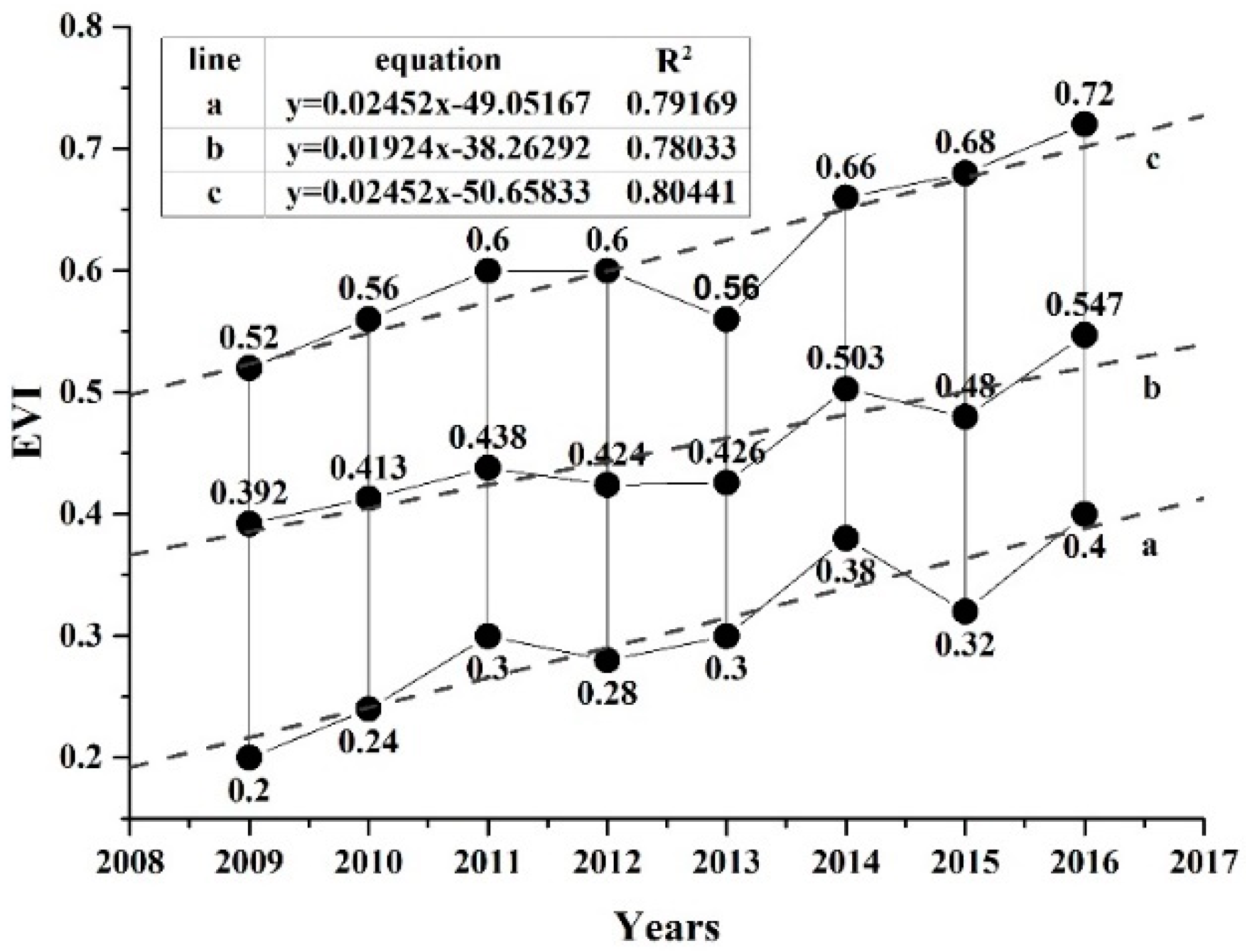
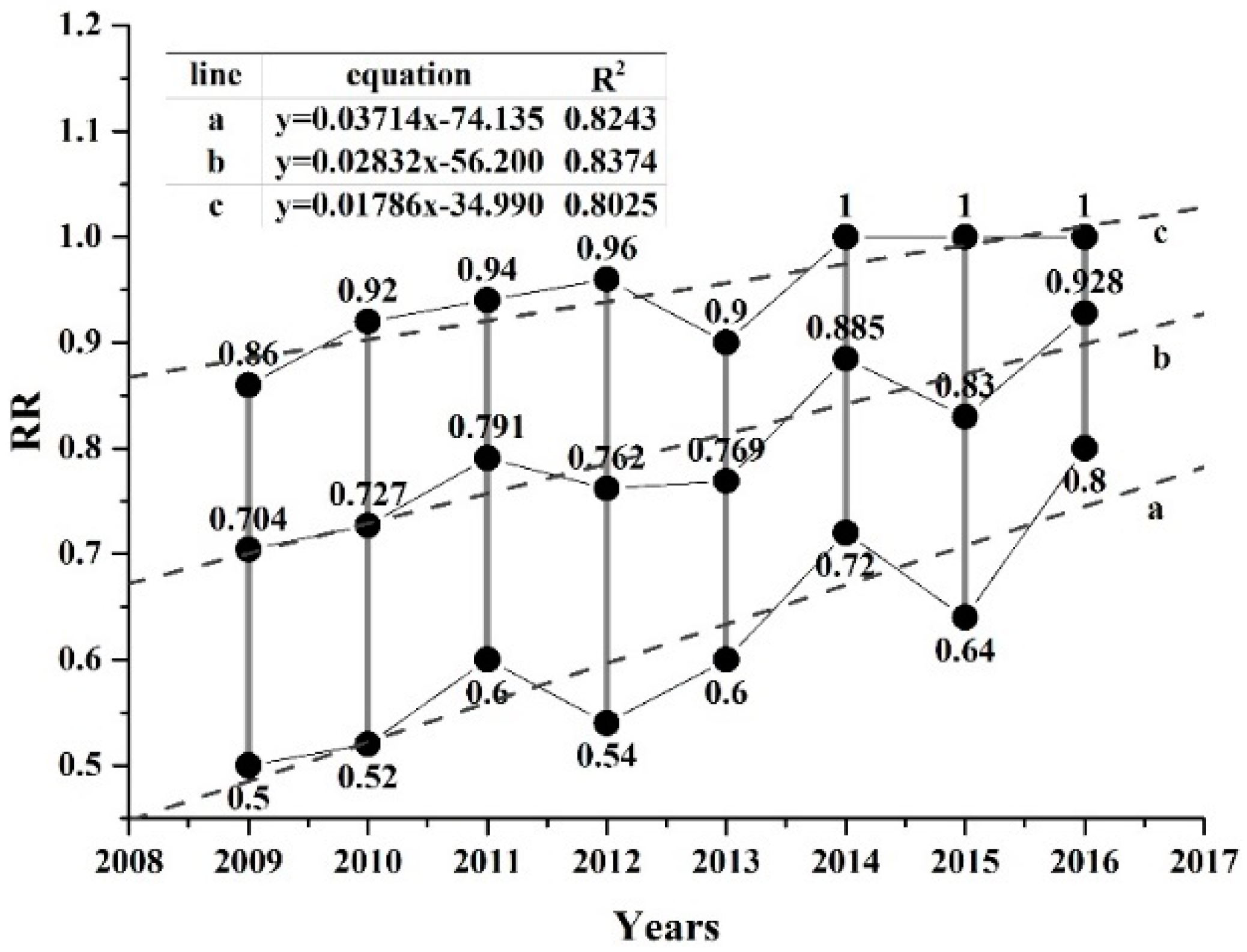
5.3. Fitting the Trend of Vegetation Recovery
5.4. Classification of Resilience
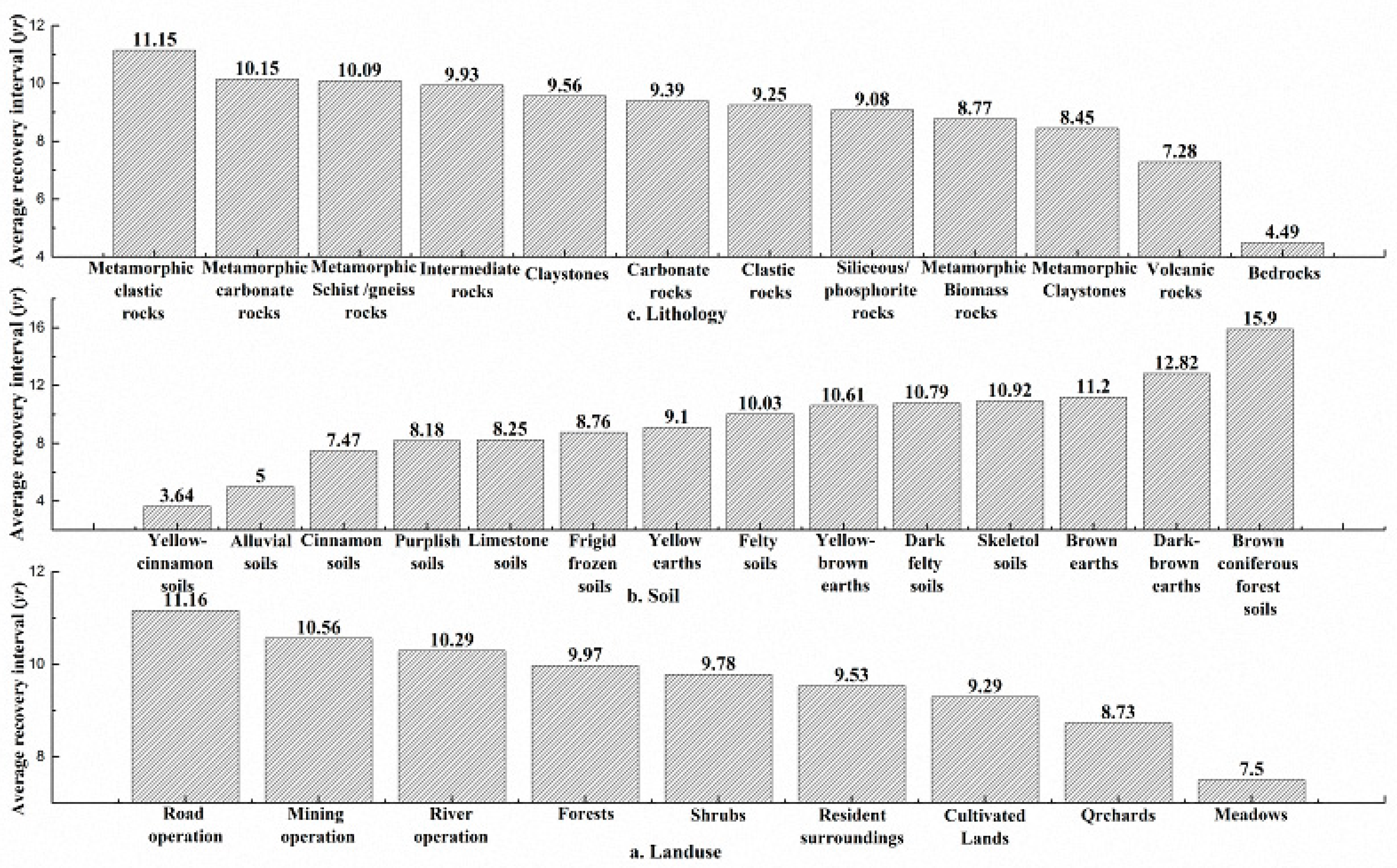
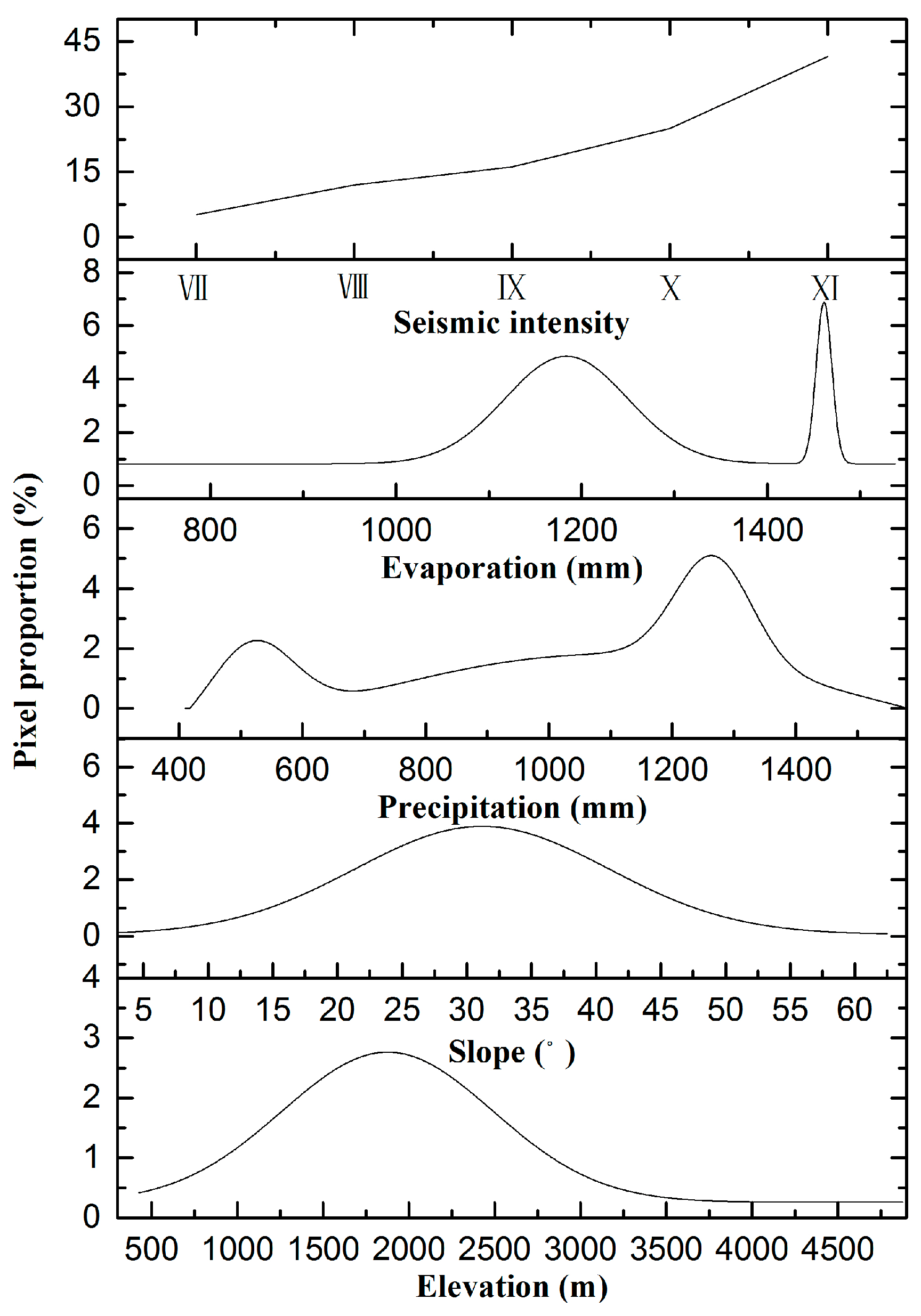
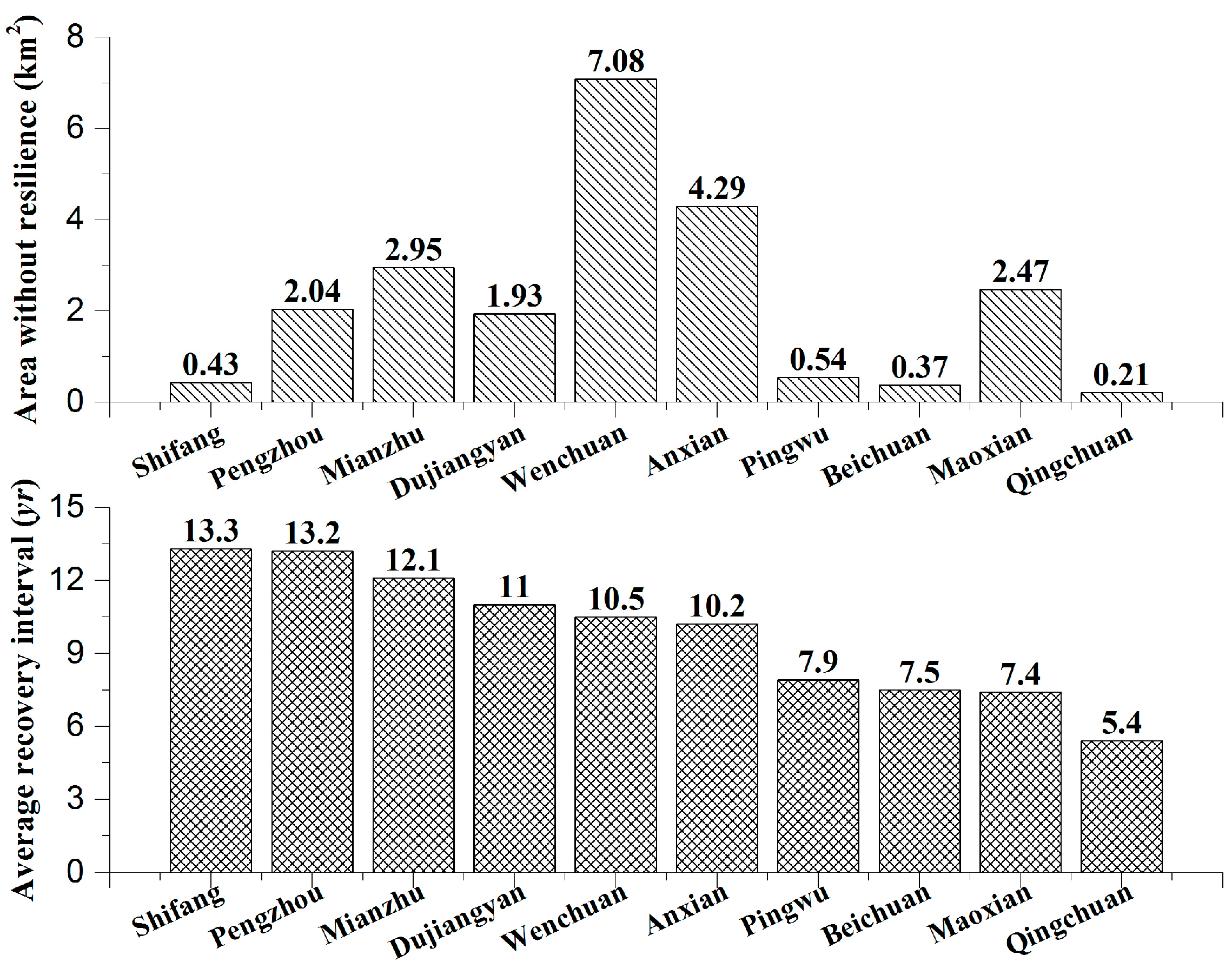
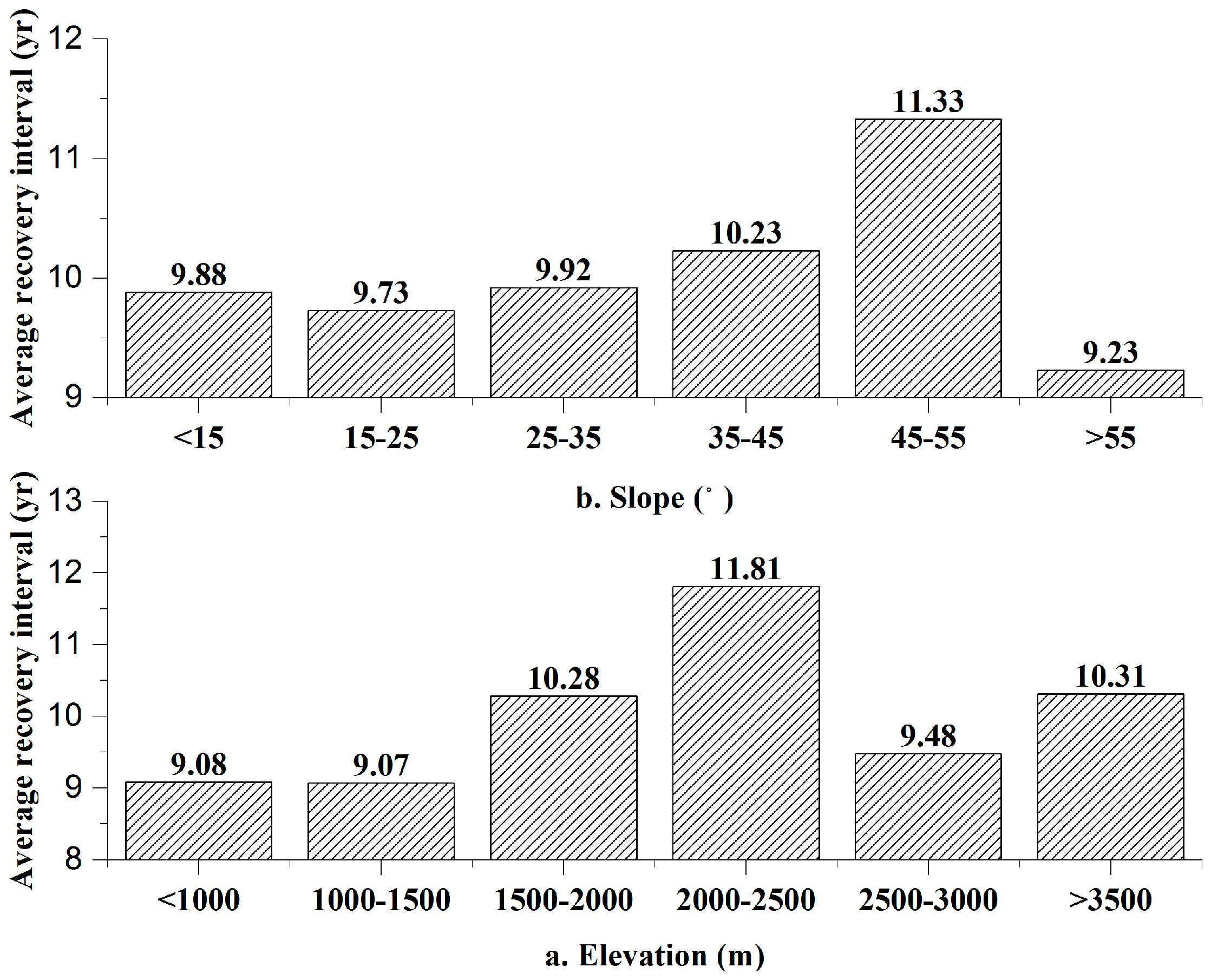
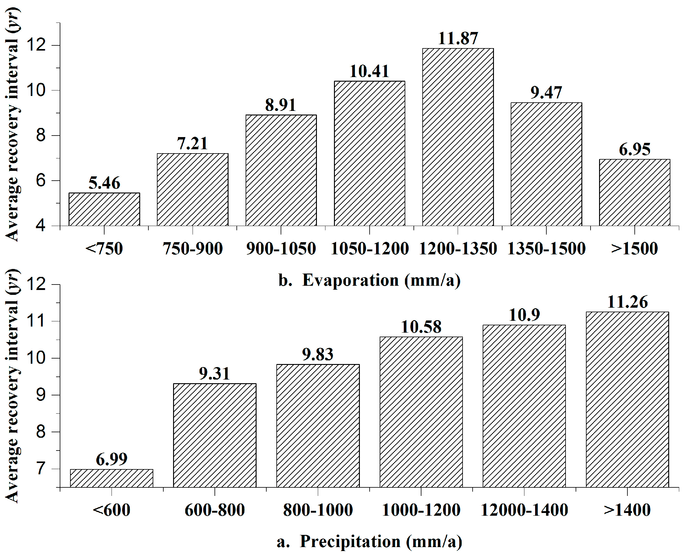
5.5. Spatial Heterogeneity in Resilience and Its Influencing Factors
6. Discussion
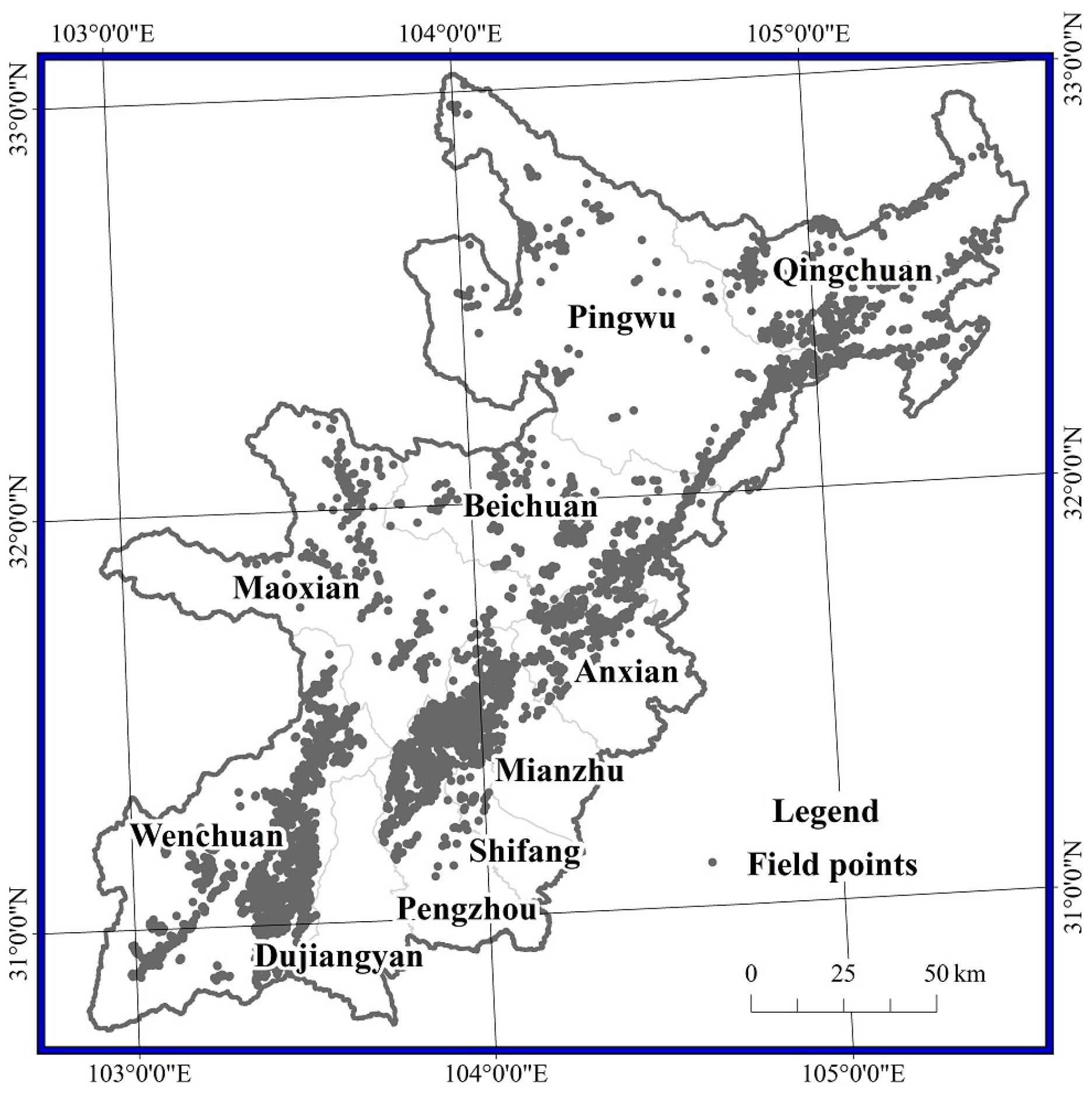
6.1. Validation of the Damaged Area Estimate
6.2. Resilience Comparison
6.3. Innovation
6.4. Uncertainty
7. Conclusions
Acknowledgments
Author Contributions
Conflicts of Interest
References
- Holling, C.S. Resilience and stability of ecological systems. Annu. Rev. Ecol. Syst. 1973, 4, 1–23. [Google Scholar] [CrossRef]
- Holling, C.S. Engineering resilience versus ecological resilience. In Engineering within Ecological Constraints; National Academy: Washington, DC, USA, 1996; pp. 31–43. [Google Scholar]
- Pimm, S.L. The complexity and stability of ecosystems. Nature 1984, 307, 321–326. [Google Scholar] [CrossRef]
- Brand, F.S.; Jax, K. Focusing the meaning(s) of resilience: Resilience as a descriptive concept and a boundary object. Ecol. Soc. 2007, 12, 181–194. [Google Scholar] [CrossRef]
- Mumby, P.J.; Chollett, I.; Bozec, Y.-M.; Wolff, N.H. Ecological resilience, robustness and vulnerability: How do these concepts benefit ecosystem management? Curr. Opin. Environ. Sustain. 2014, 7, 22–27. [Google Scholar] [CrossRef]
- Walker, B.; Salt, D. Resilience Thinking; Island Press: Washington, DC, USA, 2006. [Google Scholar]
- Folke, C.; Carpenter, S.R.; Walker, B.; Scheffer, M. Resilience thinking: Integrating resilience, adaptability and transformability. Ecol. Soc. 2010, 15, 299–305. [Google Scholar]
- Strunz, S. Is conceptual vagueness an asset? Arguments from philosophy of science applied to the concept of resilience. Ecol. Econ. 2012, 76, 112–118. [Google Scholar] [CrossRef]
- Xu, L.; Marinova, D. Resilience thinking: A bibliometric analysis of socio-ecological research. Scientometrics 2013, 96, 911–927. [Google Scholar] [CrossRef]
- Rist, L.; Moen, J. Sustainability in forest management and a new role for resilience thinking. For. Ecol. Manag. 2013, 310, 416–427. [Google Scholar] [CrossRef]
- Sterk, M.; Gort, G.; Klimkowska, A.; van Ruijven, J.; van Teeffelen, A.J.A.; Wamelink, G.W.W. Assess ecosystem resilience: Linking response and effect traits to environmental variability. Ecol. Indic. 2013, 30, 21–27. [Google Scholar] [CrossRef]
- Johnstone, J.F.; Walker, L.R.; Fastie, C.L.; Walker, L.R. Linking Deterministic and Stochastic Processes of Succession to Understand Drivers of Ecological Resilience. In Proceedings of the 97th ESA Annual Convention, Portland, OR, USA, 5 August 2012.
- Reggiani, A.; De Graaff, T.; Nijkamp, P. Resilience: An evolutionary approach to spatial economic systems. Netw. Spat. Econ. 2002, 2, 211–229. [Google Scholar] [CrossRef]
- Carpenter, S.R.; Walker, B.; Anderies, J.M.; Abel, N. From metaphor to measurement: Resilience of what to what? Ecosystems 2001, 4, 765–781. [Google Scholar] [CrossRef]
- Karr, J.R.; Thomas, T. Economics, ecology, and environmental quality. Ecol. Appl. 1996, 6, 31–32. [Google Scholar] [CrossRef]
- Frazier, T.G.; Thompson, C.M.; Dezzani, R.J.; Butsick, D. Spatial and temporal quantification of resilience at the community scale. Appl. Geogr. 2013, 42, 95–107. [Google Scholar] [CrossRef]
- Lake, P.S. Resistance, resilience and restoration. Ecol. Manag. Restor. 2013, 14, 20–24. [Google Scholar] [CrossRef]
- Perz, S.G.; Muñoz-Carpena, R.; Kiker, G.; Holt, R.D. Evaluating ecological resilience with global sensitivity and uncertainty analysis. Ecol. Model. 2013, 263, 174–186. [Google Scholar] [CrossRef]
- Ebisudani, M.; Tokai, A. Resilience: Ecological and Engineering Perspectives Present Status and Future Consideration Referring on Two Case Studies in U.S.; The Society for Risk Analysis Japan, Kyoto University: Kyoto, Japan, 2014. [Google Scholar]
- Hofmann, M. Resilience. A Formal Approach to an Ambiguous Concept. Ph.D. Thesis, Freie Universität Berlin, Berlin, Germany, 2007. [Google Scholar]
- Wissel, C. A universal law of the characteristic return time near thresholds. Oecologia 1984, 65, 101–107. [Google Scholar] [CrossRef]
- Scheffer, M.; Bascompte, J.; Brock, W.A.; Brovkin, V.; Carpenter, S.R.; Dakos, V.; Held, H.; Nes, E.H.V.; Rietkerk, M.; Sugihara, G. Early-warning signals for critical transitions. Nature 2009, 461, 53–59. [Google Scholar] [CrossRef] [PubMed]
- Dakos, V.; van Nes, E.; Donangelo, R.; Fort, H.; Scheffer, M. Spatial correlation as leading indicator of catastrophic shifts. Theor. Ecol. 2010, 3, 163–174. [Google Scholar] [CrossRef]
- Bisson, M.; Fornaciai, A.; Coli, A.; Mazzarini, F.; Pareschi, M.T. The vegetation resilience after fire (VRAF) index: Development, implementation and an illustration from central Italy. Int. J. Appl. Earth Obs. Geoinform. 2008, 10, 312–329. [Google Scholar] [CrossRef]
- Robert, A.V.L.; Kirk, E.L.; James, A.K. Modeling the suitability of potential wetland mitigation sites with a geographic information. Environ. Manag. 2004, 33, 368–375. [Google Scholar]
- Lanfredi, M.; Simoniello, T.; Macchiato, M. Temporal persistence in vegetation cover changes observed from satellite: Development of an estimation procedure in the test site of the Mediterranean Italy. Remote Sens. Environ. 2004, 93, 565–576. [Google Scholar] [CrossRef]
- Coppola, R.; Cuomo, V.; D’Emilio, M.; Lanfredi, M.; Liberti, M.; Macchiato, M.; Simoniello, T. Terrestrial vegetation cover activity as a problem of fluctuating surfaces. Int. J. Mod. Phys. B 2009, 23, 5444–5452. [Google Scholar] [CrossRef]
- Simoniello, T.; Lanfredi, M.; Liberti, M.; Coppola, R.; Macchiato, M. Estimation of vegetation cover resilience from satellite time series. Hydrol. Earth Syst. Sci. 2008, 12, 1053–1064. [Google Scholar] [CrossRef]
- Vitale, M.; Capogna, F.; Manes, F. Resilience assessment on phillyearsea angustifolia l. Maquis undergone to experimental fire through a big-leaf modelling approach. Ecol. Model. 2007, 203, 387–394. [Google Scholar] [CrossRef]
- Cui, P.; Lin, Y.-M.; Chen, C. Destruction of vegetation due to geo-hazards and its environmental impacts in the Wenchuan earthquake areas. Ecol. Eng. 2012, 44, 61–69. [Google Scholar] [CrossRef]
- Lu, T.; Zeng, H.; Luo, Y.; Wang, Q.; Shi, F.; Sun, G.; Wu, Y.; Wu, N. Monitoring vegetation recovery after China’s may 2008 Wenchuan earthquake using Landsat tm time-series data: A case study in Mao county. Ecol. Res. 2012, 27, 955–966. [Google Scholar] [CrossRef]
- Hou, P.; Wang, Q.; Yang, Y.; Jiang, W.; Yang, B.; Chen, Q.; Yuan, L.; Kong, F.; Chen, X.; Wang, G. Spatio-temporal features of vegetation restoration and variation after the Wenchuan earthquake with satellite images. J. Appl. Remote Sens. 2014, 8, 2731–2743. [Google Scholar]
- Wang, M.; Yang, W.; Shi, P.; Xu, C.; Liu, L. Diagnosis of vegetation recovery in mountainous regions after the Wenchuan earthquake. IEEE J. Sel. Top. Appl. Earth Obs. Remote Sens. 2014, 7, 3029–3037. [Google Scholar] [CrossRef]
- Zhang, J.; Hull, V.; Huang, J.; Yang, W.; Zhou, S.; Xu, W.; Huang, Y.; Ouyang, Z.; Zhang, H.; Liu, J. Natural recovery and restoration in giant panda habitat after the Wenchuan earthquake. For. Ecol. Manag. 2014, 319, 1–9. [Google Scholar] [CrossRef]
- Jiang, W.G.; Jia, K.; Wu, J.J.; Tang, Z.H.; Wang, W.J.; Liu, X.F. Evaluating the vegetation recovery in the damage area of Wenchuan earthquake using MODIS data. Remote Sens. 2015, 7, 8757–8778. [Google Scholar] [CrossRef]
- Pan, Q.; Zhang, Q.J.; Liang, X.U. Basing on RS & GIS monitoring of ecological restoration in very disaster-hit area of Wenchuan earthquake—A case study of Dujiangyan city. Sichuan Environ. 2012, 31, 29–33. [Google Scholar]
- Gu, Y.; Wylie, B.K.; Howard, D.M.; Phuyal, K.P.; Ji, L. Ndvi saturation adjustment: A new approach for improving cropland performance estimates in the greater Platte river basin, USA. Ecol. Indic. 2013, 30, 1–6. [Google Scholar] [CrossRef]
- Li, Z.; Li, X.; Wei, D.; Xu, X.; Wang, H. An assessment of correlation on MODIS-NDVI and EVI with natural vegetation coverage in northern Hebei province, China. Procedia Environ. Sci. 2010, 2, 964–969. [Google Scholar] [CrossRef]
- Taddei, R. Maximum value interpolated (mvi): A maximum value composite method improvement in vegetation index profiles analysis. Int. J. Remote Sens. 1997, 18, 2365–2370. [Google Scholar] [CrossRef]
- Lin, C.-Y.; Lo, H.-M.; Chou, W.-C.; Lin, W.-T. Vegetation recovery assessment at the Jou-Jou mountain landslide area caused by the 921 earthquake in central Taiwan. Ecol. Model. 2004, 176, 75–81. [Google Scholar] [CrossRef]
- Lin, W.-T.; Lin, C.-Y.; Chou, W.-C. Assessment of vegetation recovery and soil erosion at landslides caused by a catastrophic earthquake: A case study in central Taiwan. Ecol. Eng. 2006, 28, 79–89. [Google Scholar] [CrossRef]
- Yang, W.T.; Qi, W.W. Spatial-temporal dynamic monitoring of vegetation recovery after the Wenchuan earthquake. IEEE J. Sel. Top. Appl. Earth Obs. Remote Sens. 2016, PP, 1–9. [Google Scholar] [CrossRef]
- Xu, C.; Xu, X. Comment on “Spatial distribution analysis of landslides triggered by 2008.5.12 Wenchuan earthquake, China” by Shengwen Qi, Qiang Xu, Hengxing Lan, Bing Zhang, Jianyou Liu [Engineering Geology 116 (2010) 95–108]. Eng. Geol. 2012, 133–134, 40–42. [Google Scholar] [CrossRef]
- Xu, C.; Xu, X.; Yao, X.; Dai, F. Three (nearly) complete inventories of landslides triggered by the May 12, 2008 Wenchuan mw 7.9 earthquake of China and their spatial distribution statistical analysis. Landslides 2014, 11, 441–461. [Google Scholar] [CrossRef]
- Zhang, H.; Chi, T.; Fan, J.; Hu, K.; Peng, L. Spatial analysis of Wenchuan earthquake-damaged vegetation in the mountainous basins and its applications. Remote Sens. 2015, 7, 5785–5804. [Google Scholar] [CrossRef]


| Classification of Resilience | Recovery Interval | Number of Pixels | Area (km2) | Percentage of the Total Damaged Area |
|---|---|---|---|---|
| Excellent | ≤1 year | 188 | 10.09 | 2.38% |
| Good | 2–3 years | 512 | 27.48 | 6.48% |
| Moderate | 4–5 years | 376 | 20.18 | 4.76% |
| 6–8 years | 2416 | 129.65 | 30.57% | |
| Low | 9–10 years | 1535 | 82.38 | 19.43% |
| 11–20 years | 2004 | 107.54 | 25.36% | |
| Bad | 21–30 years | 301 | 16.15 | 3.81% |
| 31–50 years | 154 | 8.26 | 1.95% | |
| No resilience | >50 years | 416 | 22.32 | 5.26% |
© 2017 by the authors. Licensee MDPI, Basel, Switzerland. This article is an open access article distributed under the terms and conditions of the Creative Commons Attribution (CC BY) license ( http://creativecommons.org/licenses/by/4.0/).
Share and Cite
Liu, X.; Jiang, W.; Li, J.; Wang, W. Evaluation of the Vegetation Coverage Resilience in Areas Damaged by the Wenchuan Earthquake Based on MODIS-EVI Data. Sensors 2017, 17, 259. https://doi.org/10.3390/s17020259
Liu X, Jiang W, Li J, Wang W. Evaluation of the Vegetation Coverage Resilience in Areas Damaged by the Wenchuan Earthquake Based on MODIS-EVI Data. Sensors. 2017; 17(2):259. https://doi.org/10.3390/s17020259
Chicago/Turabian StyleLiu, Xiaofu, Weiguo Jiang, Jing Li, and Wenjie Wang. 2017. "Evaluation of the Vegetation Coverage Resilience in Areas Damaged by the Wenchuan Earthquake Based on MODIS-EVI Data" Sensors 17, no. 2: 259. https://doi.org/10.3390/s17020259