Control Design and Digital Implementation of a Fast 2-Degree-of-Freedom Translational Optical Image Stabilizer for Image Sensors in Mobile Camera Phones


Abstract
:1. Introduction
2. The OIS Model
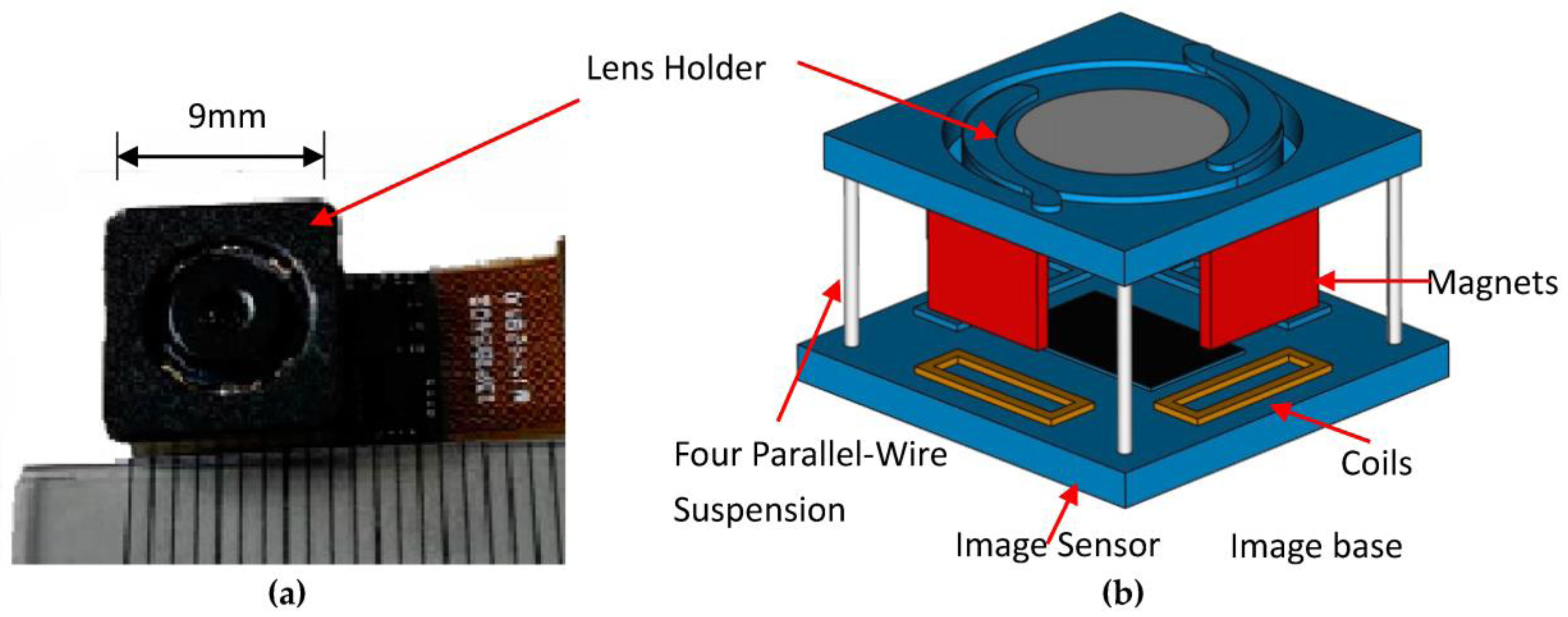
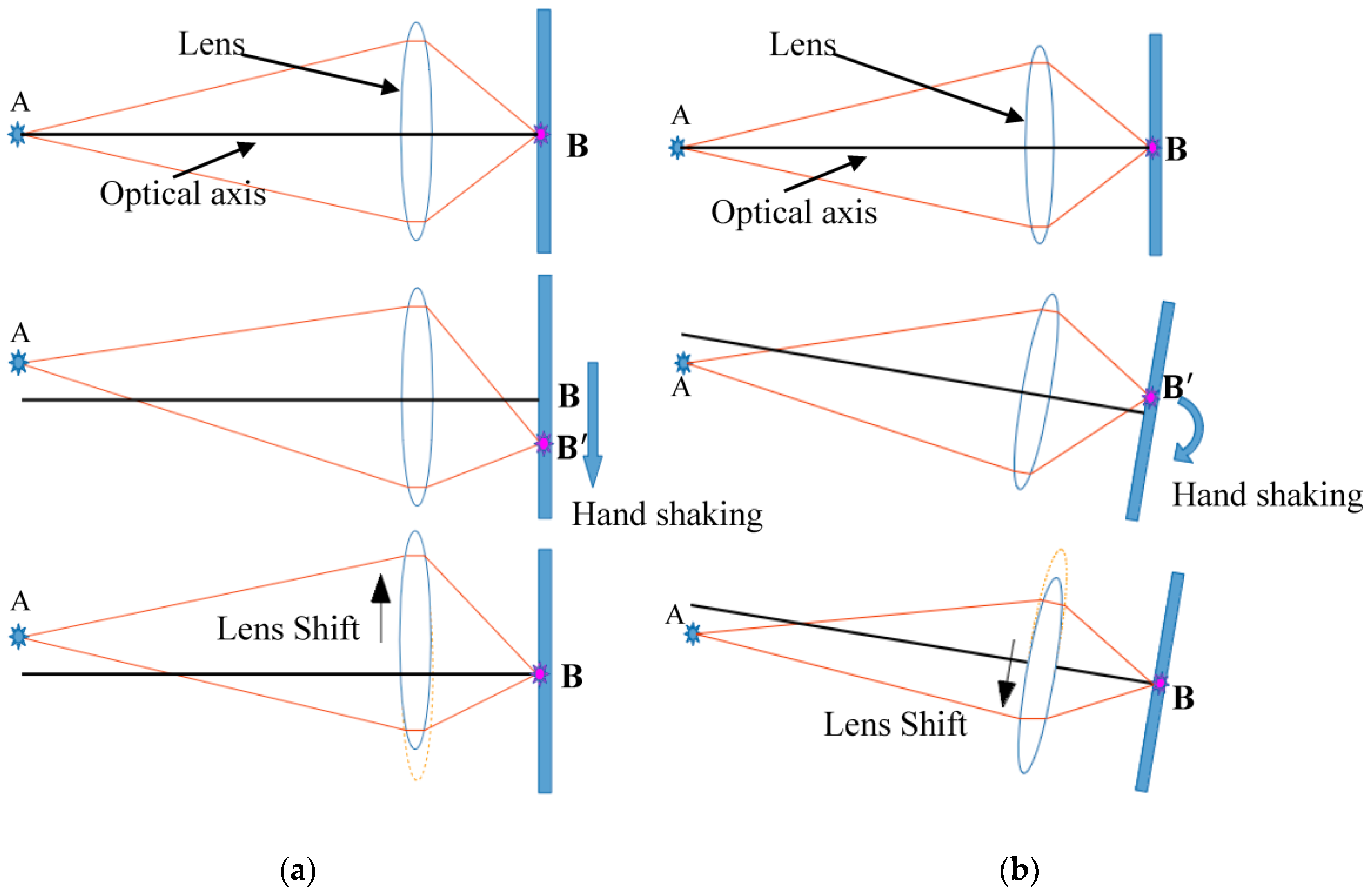
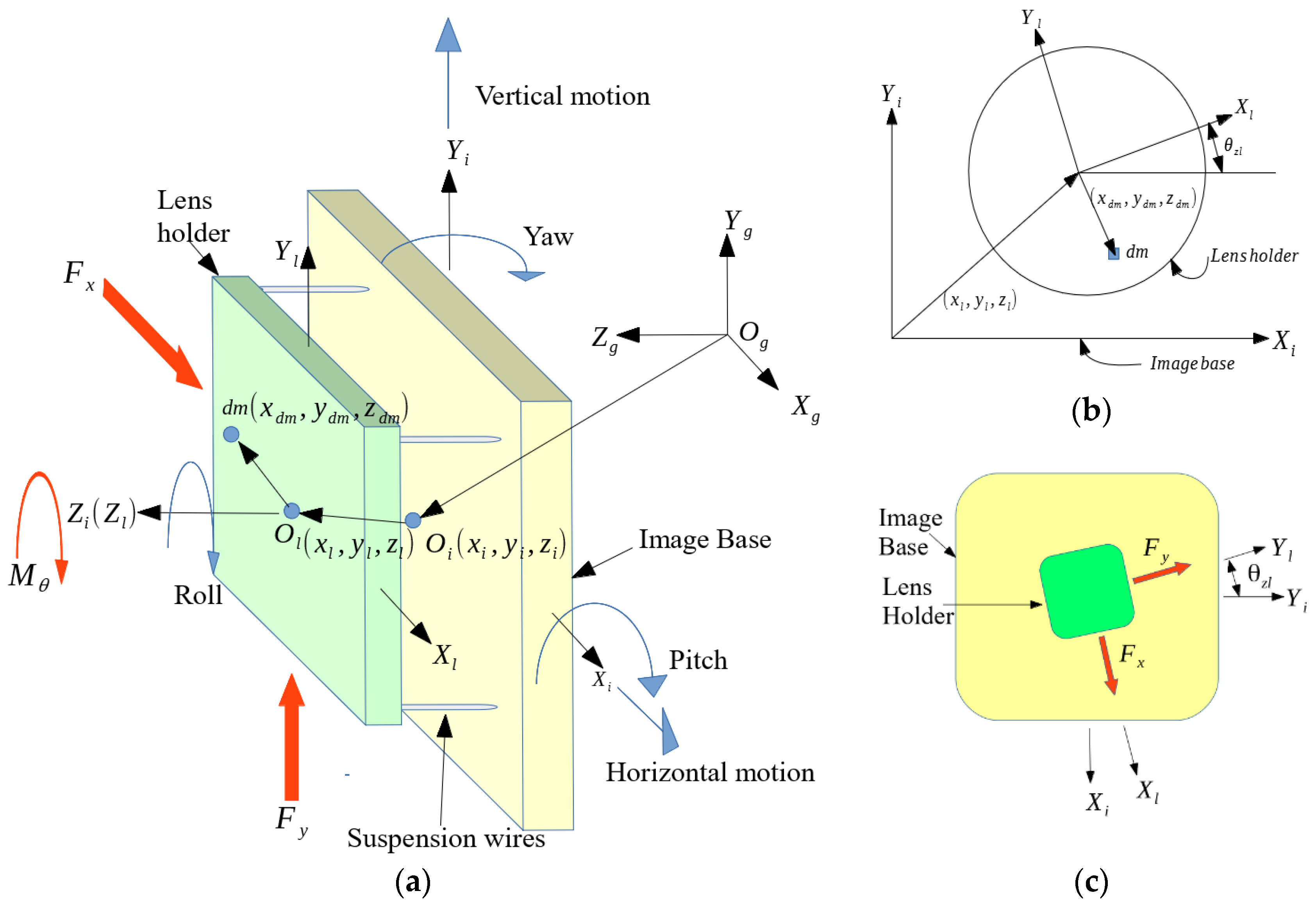
2.1. OIS Mechanism
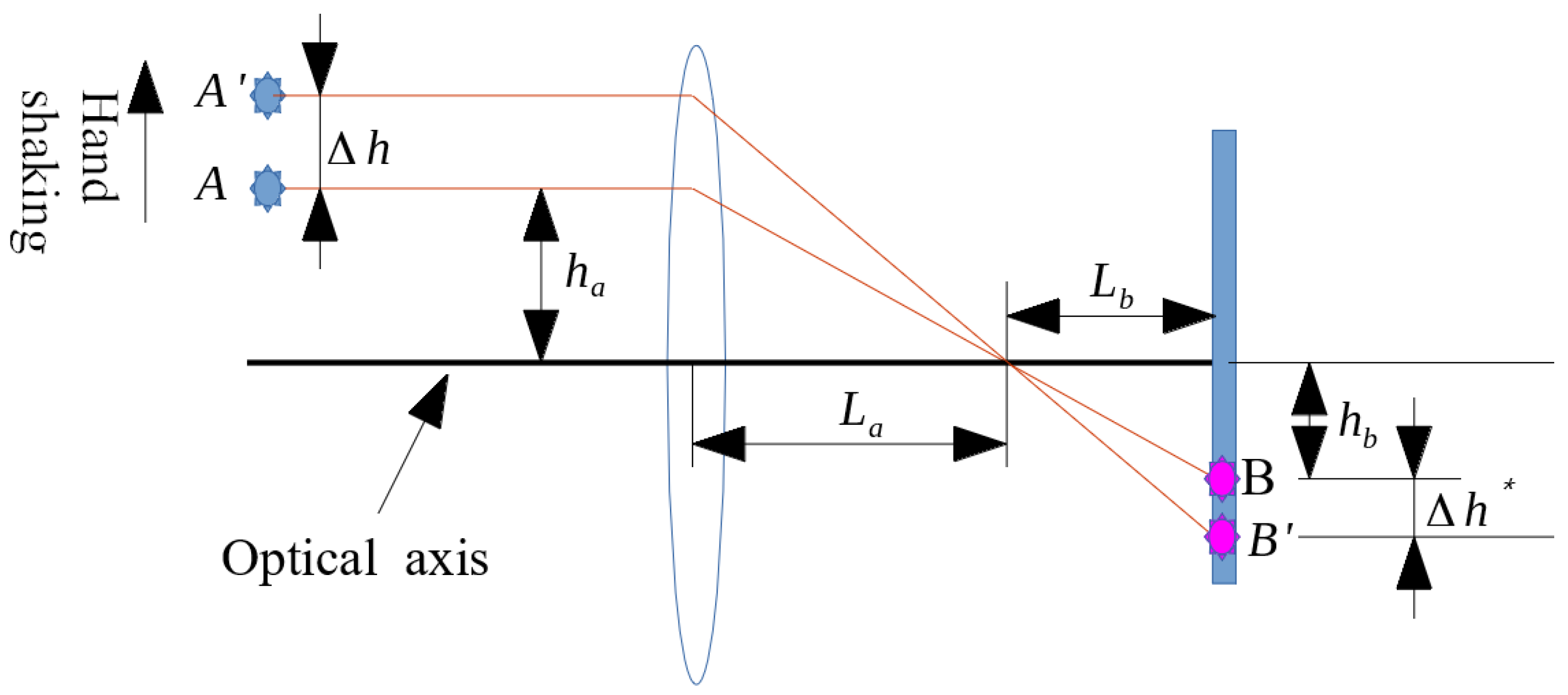
2.2. Governing Equations of OIS
3. Control Design for OIS
3.1. Control Objectives
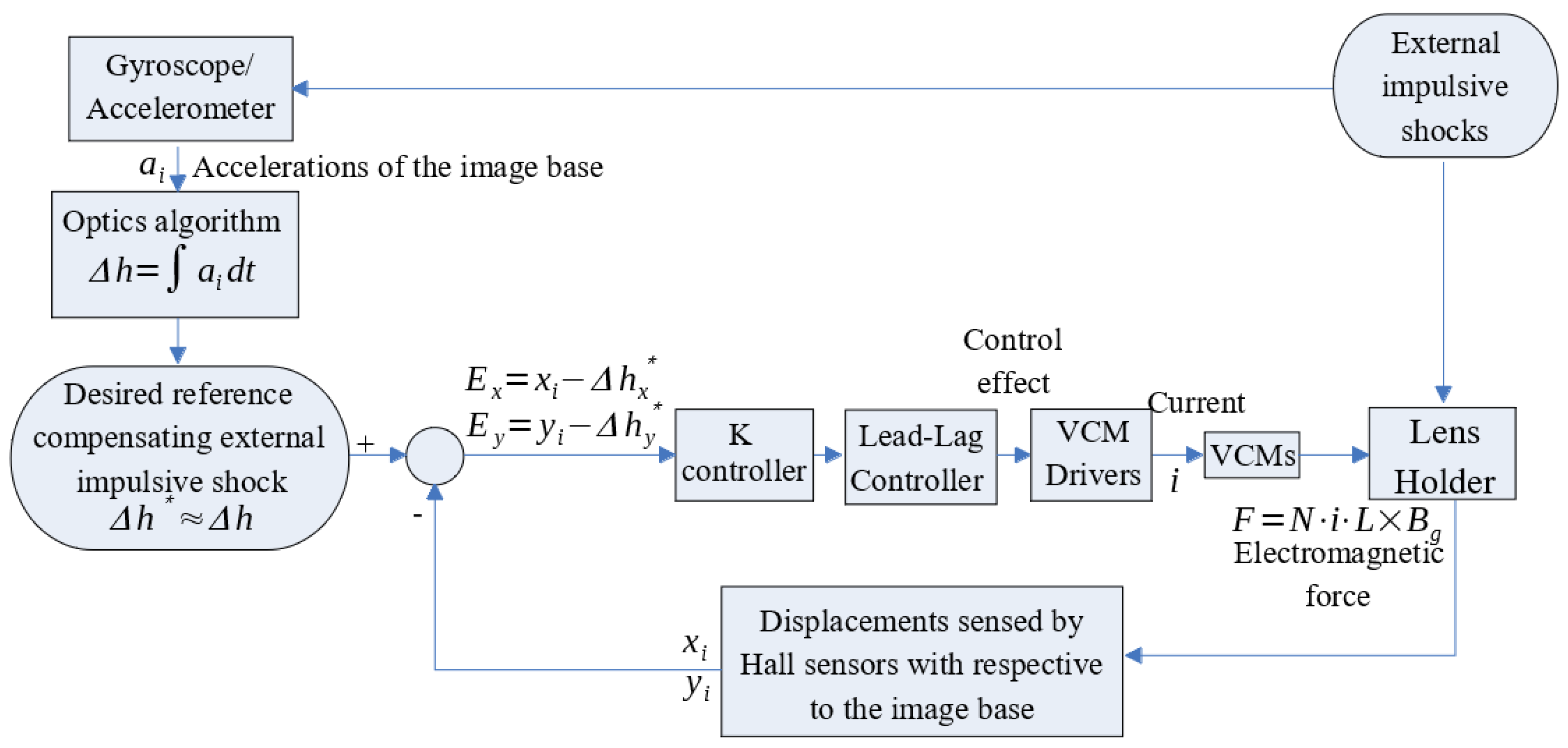
3.2. The Closed-Loop System for the OIS
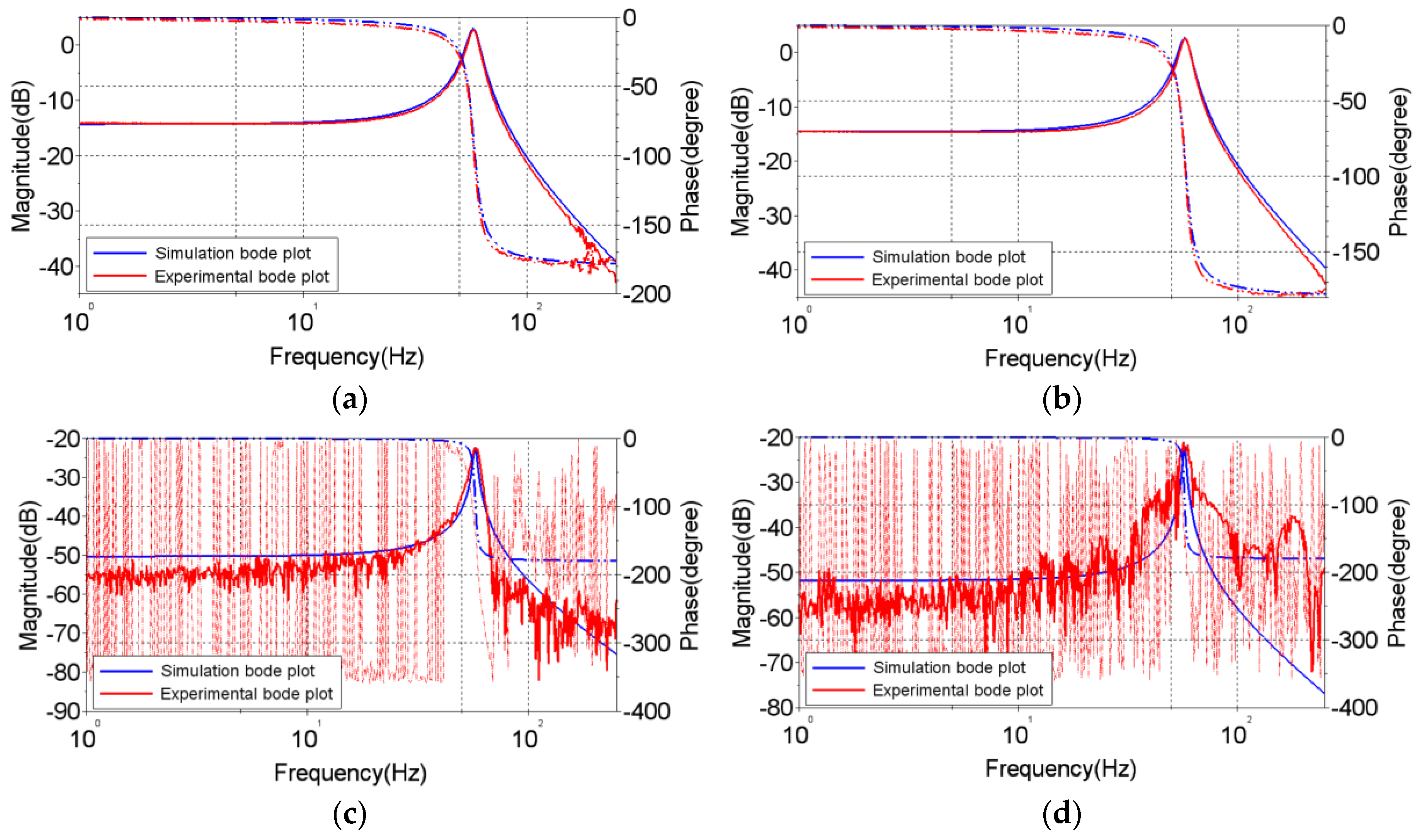
3.3. System Identification for the OIS
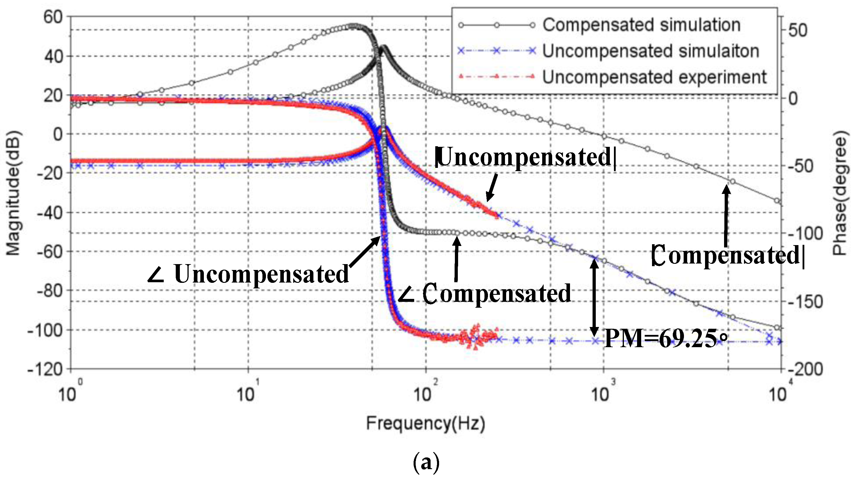
3.4. Design of a Lead-Lag Controller
4. Simulation and Experimental Results
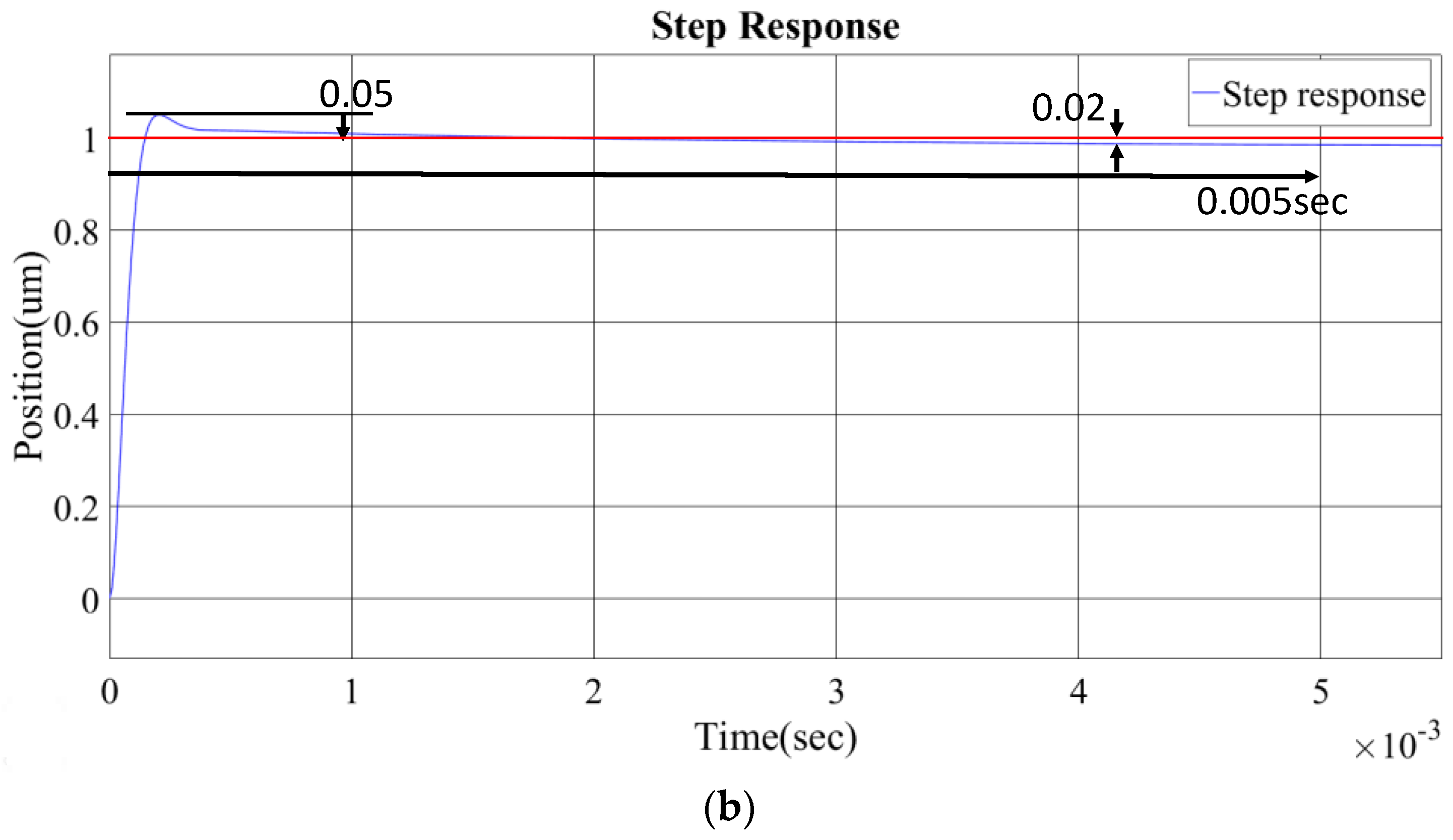
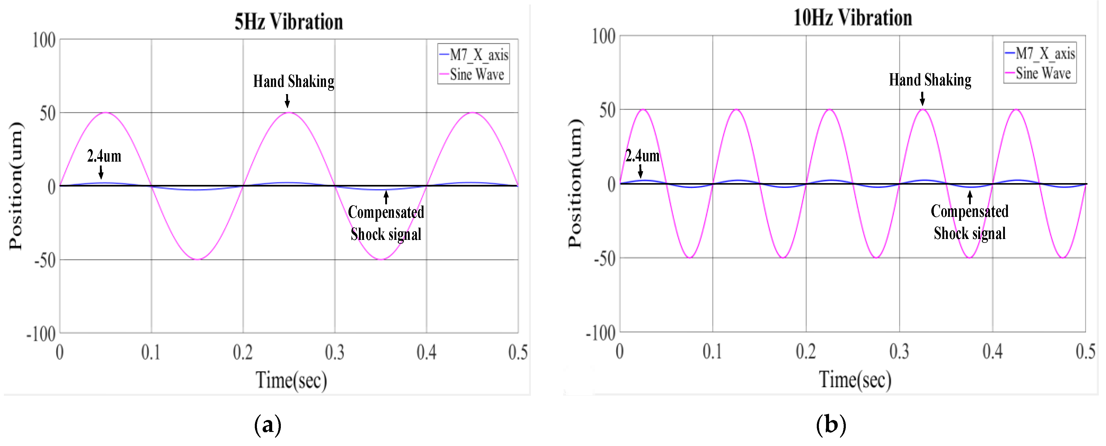
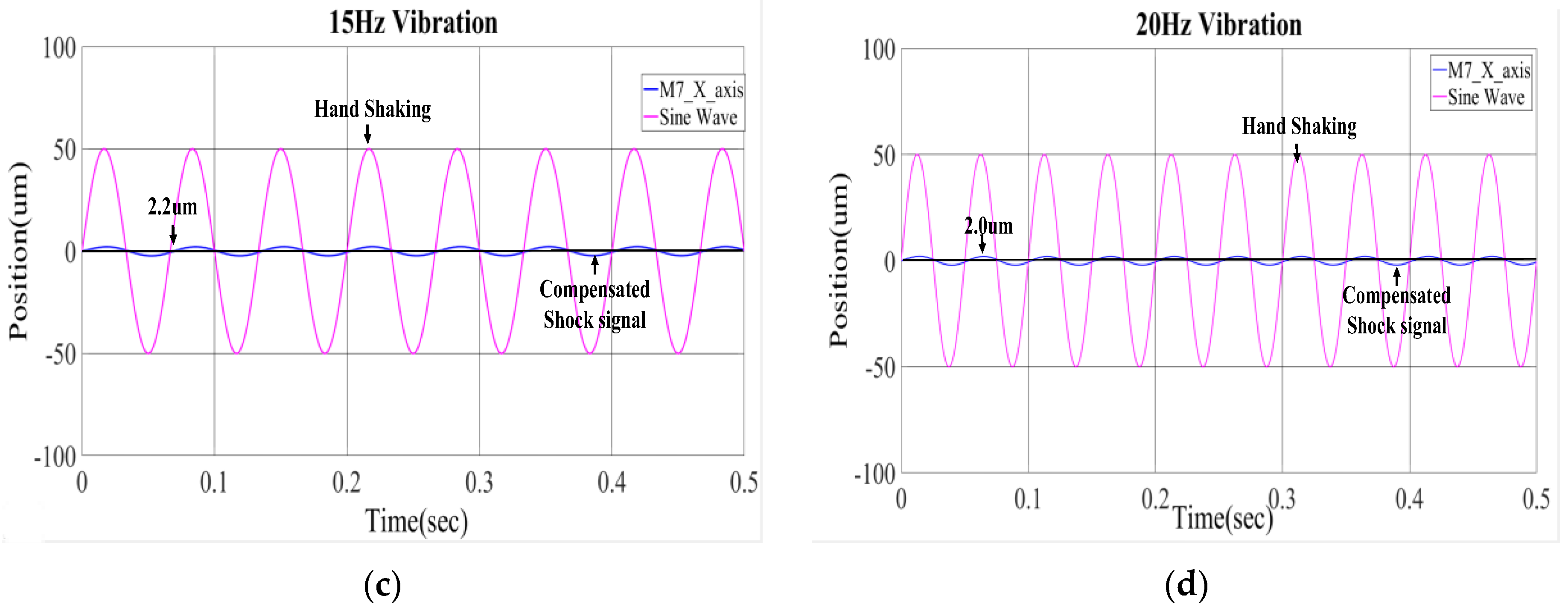
4.1. Simulation Results
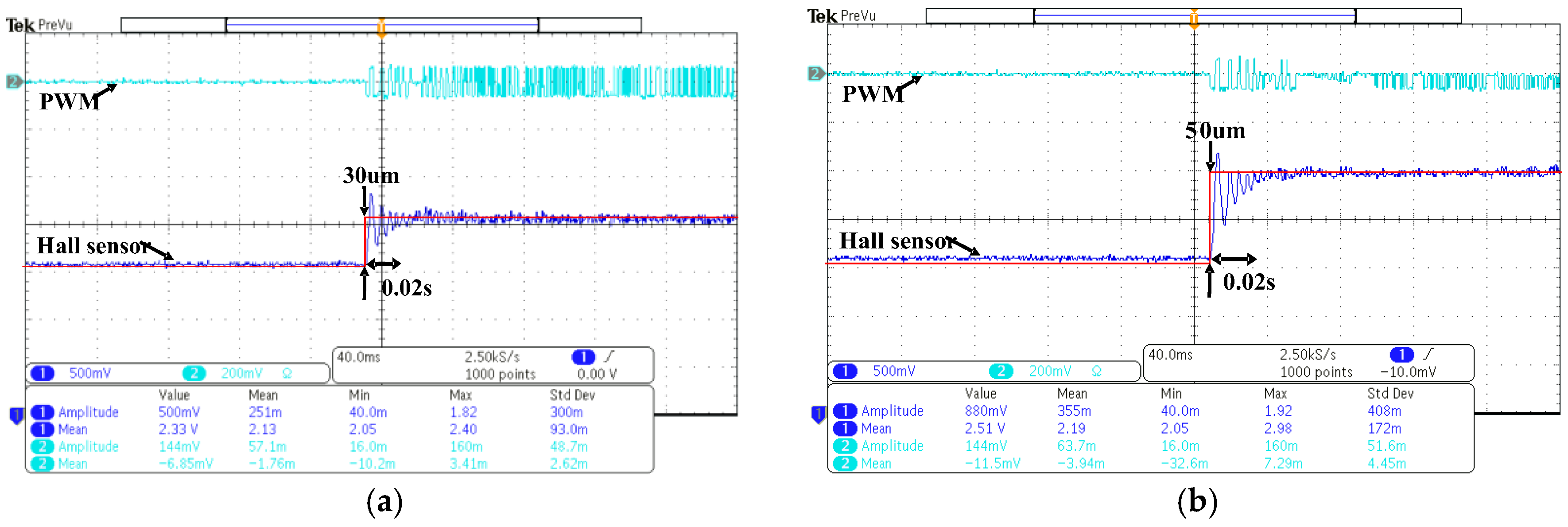
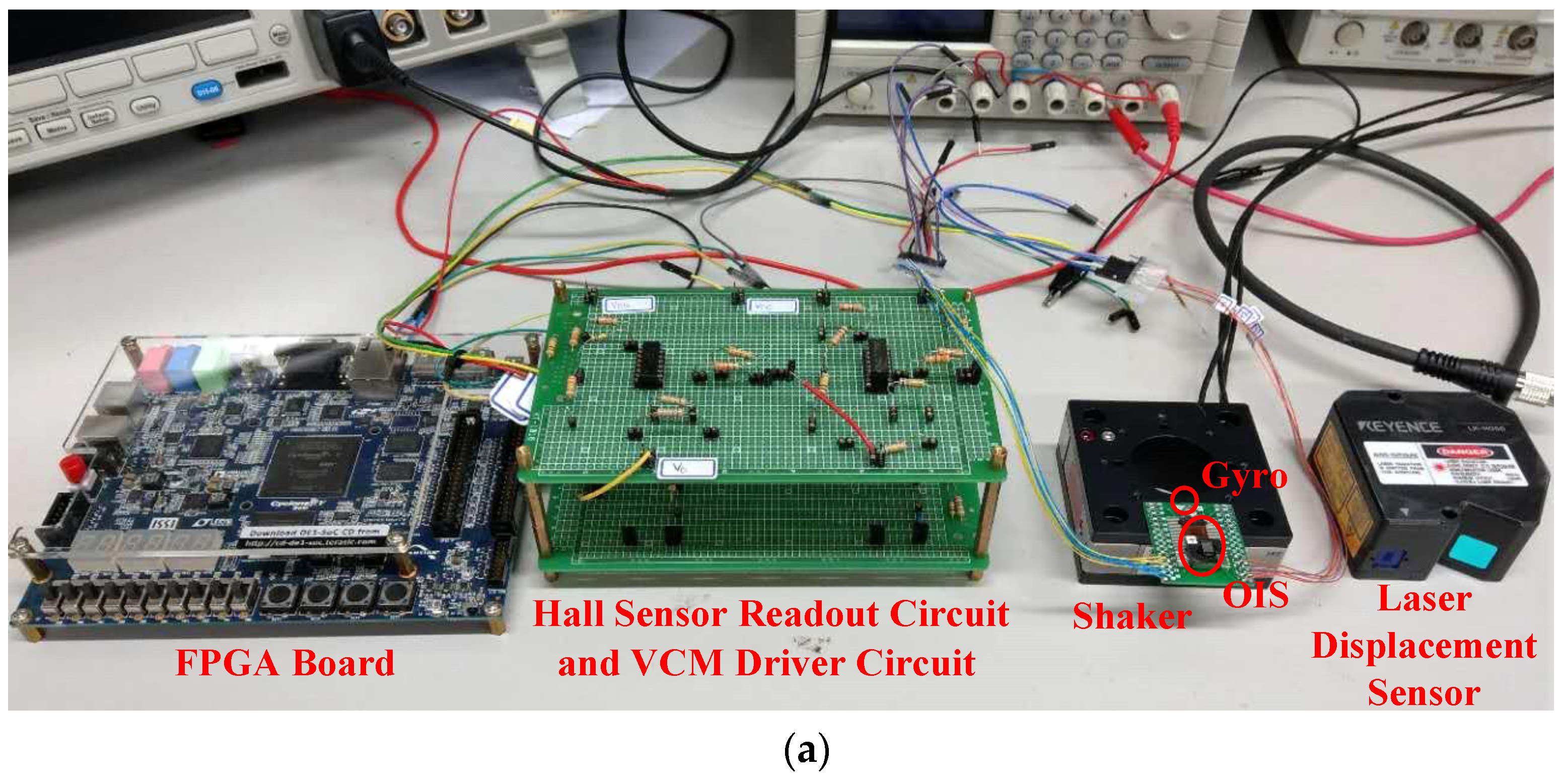
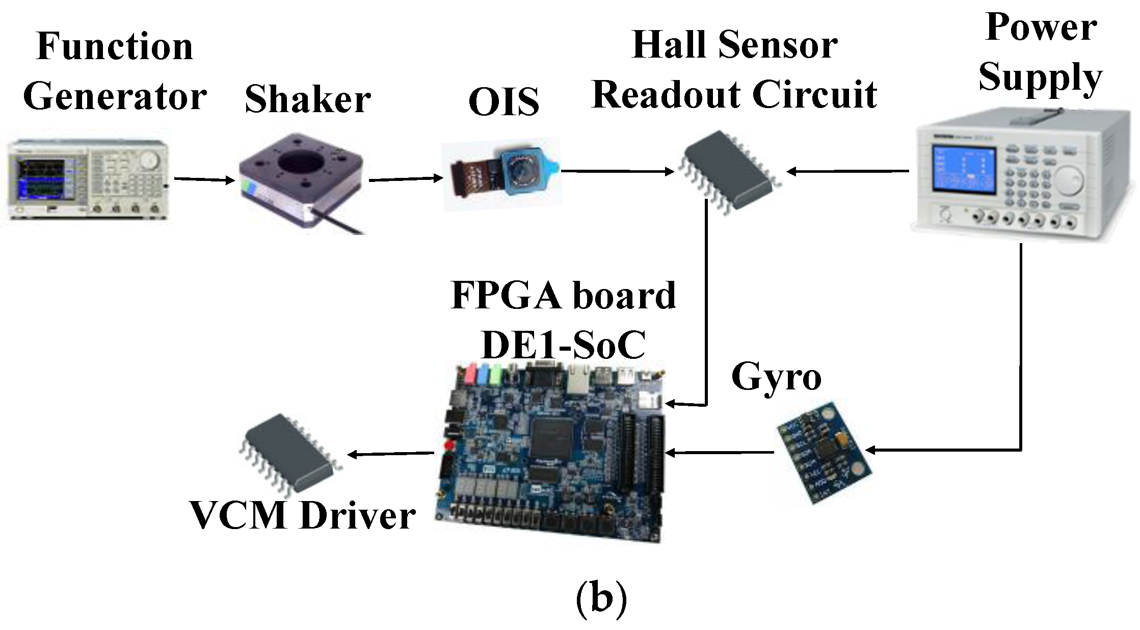
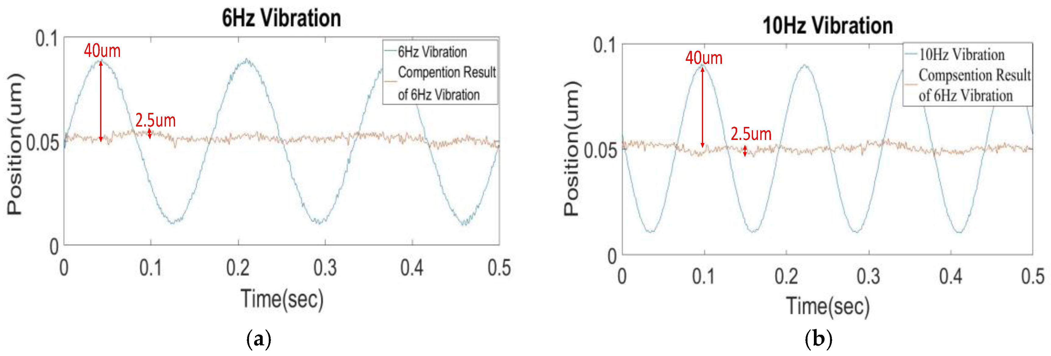
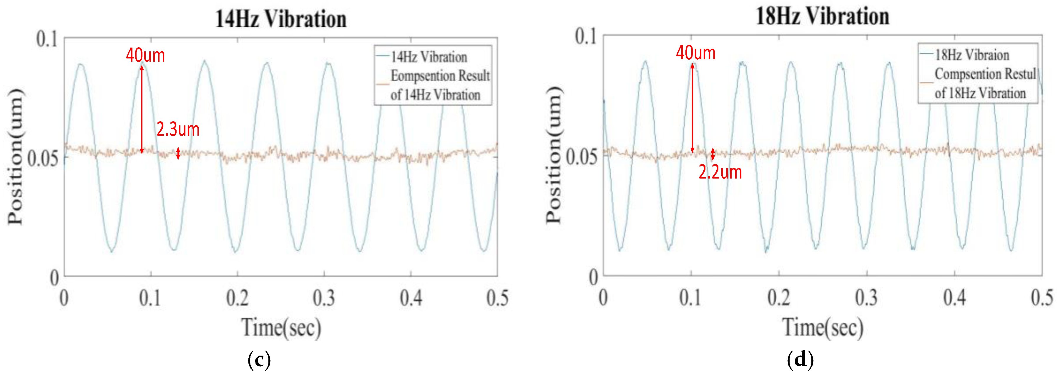
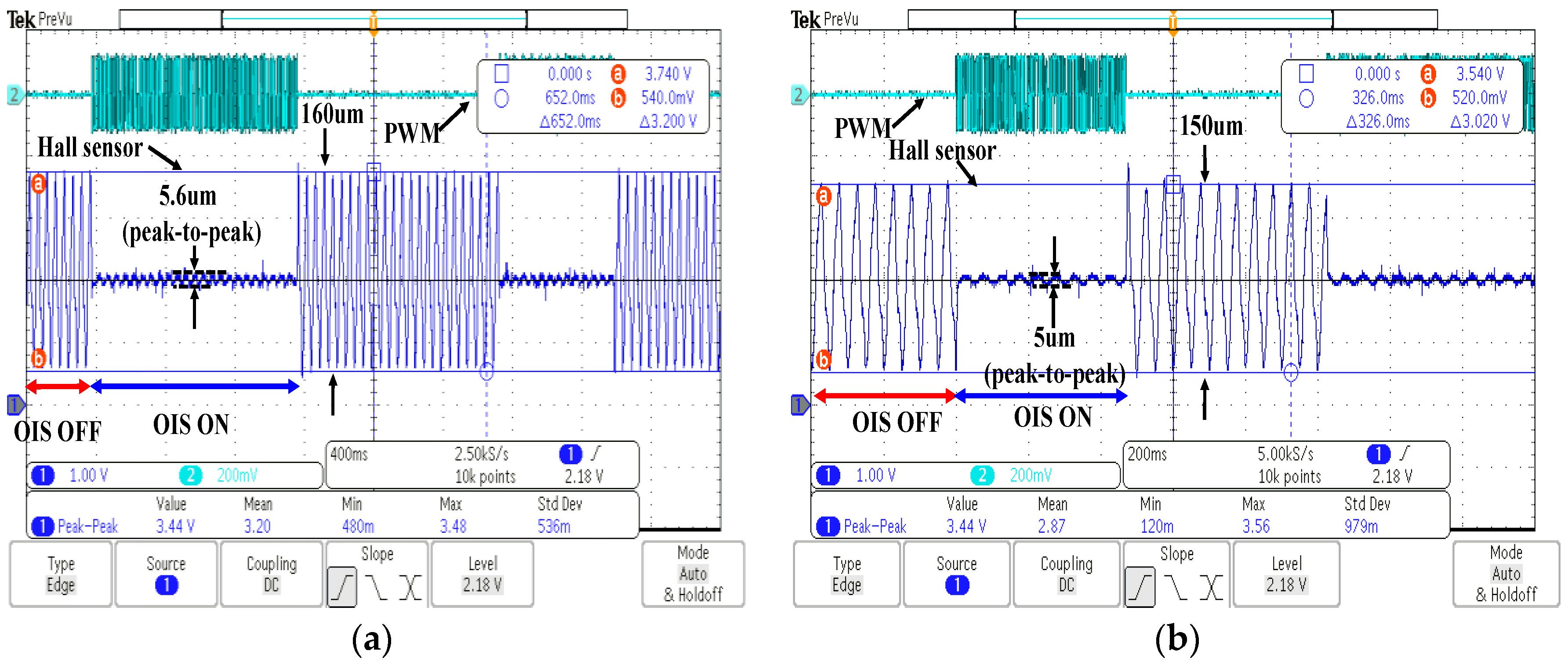
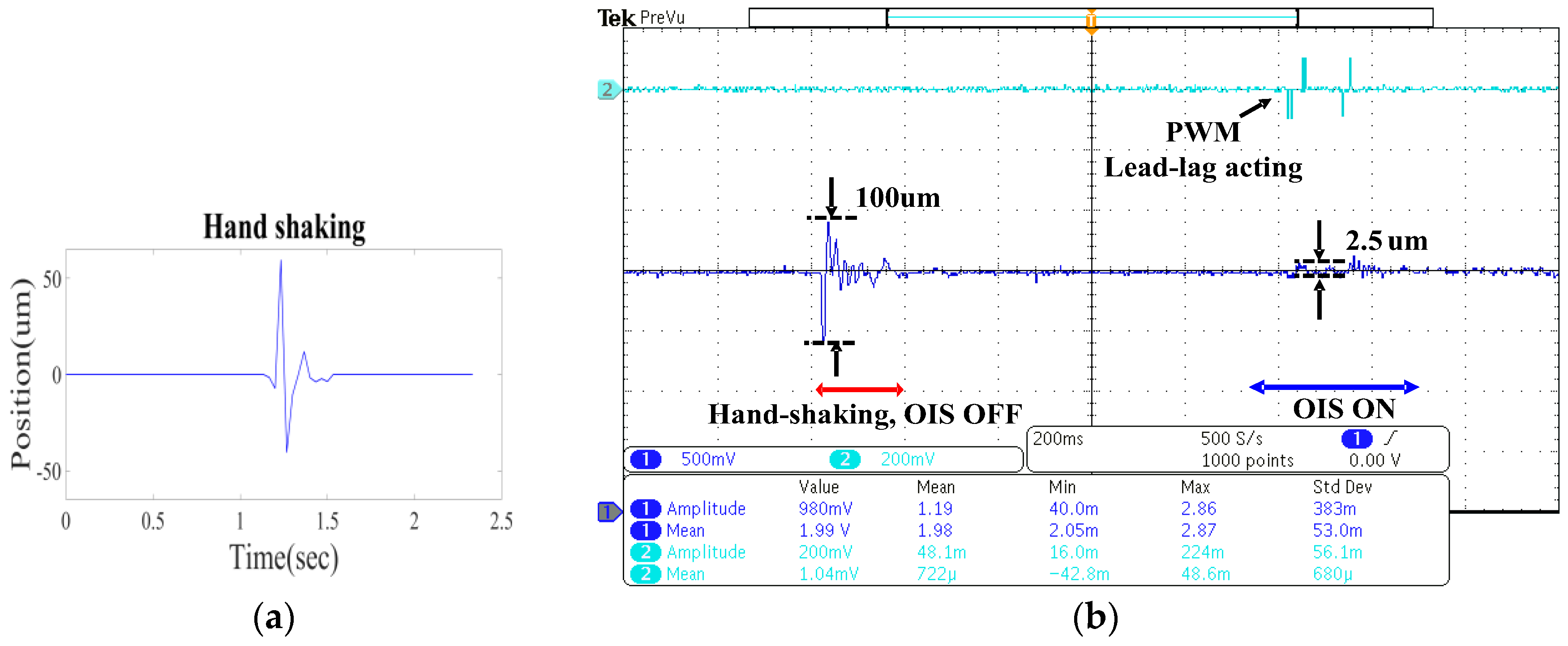
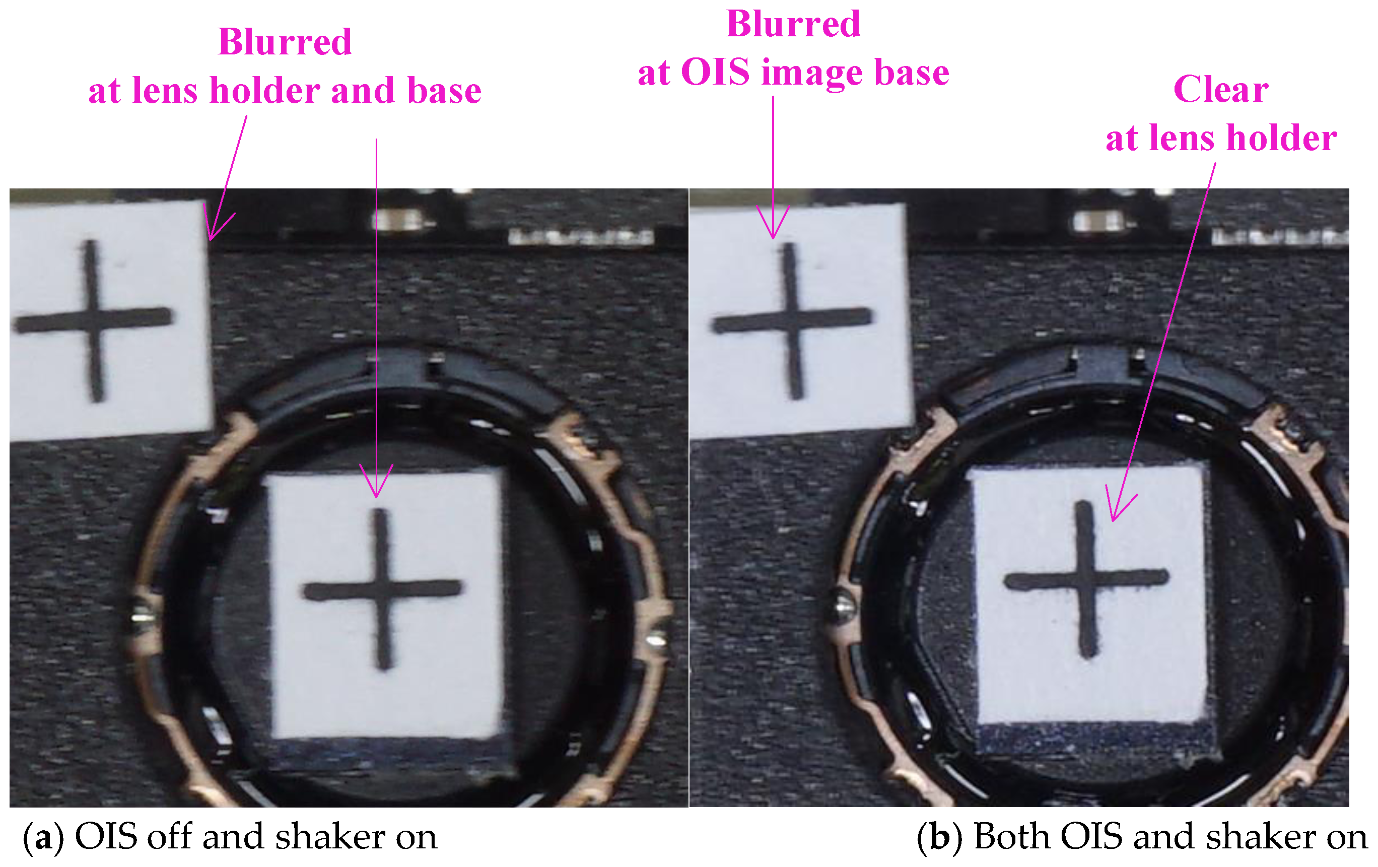
4.2. Experimental Results
5. Conclusions
Acknowledgments
Author Contributions
Conflicts of Interest
References
- Ko, S.-J.; Lee, S.-H.; Lee, K.-H. Digital image stabilizing algorithms based on bit-plane matching. IEEE Trans. Consum. Electron. 1998, 44, 617–622. [Google Scholar]
- Yeom, D.H. Optical image stabilizer for digital photographing apparatus. IEEE Trans. Consum. Electron. 2009, 55, 1028–1031. [Google Scholar] [CrossRef]
- Gasteratos, A. Active camera stabilization with a fuzzy-grey controller. Eur. J. Mech. Environ. Eng. 2009, 2, 18–20. [Google Scholar]
- Zhai, B.; Zheng, J.; Li, B. Digital image stabilization based on adaptive motion filtering with feedback correction. Multimedia Tools Appl. 2016, 75, 12173–12200. [Google Scholar] [CrossRef]
- Erturk, S. Real-Time Digital Image Stabilization Using Kalman Filters. Real-Time Images 2002, 8, 317–328. [Google Scholar] [CrossRef]
- Lamża, A.; Wróbel, Z. New Efficient Method of Digital Video Stabilization for In-Car Camera Multimedia Communications, Services and Security. MCSS 2012, 180–187. [Google Scholar]
- Chang, J.-Y.; Hu, W.-F.; Cheng, M.-H.; Chang, B.-S. Digital image translational and rotational motion stabilization using optical low technique. IEEE Trans. Consum. Electron. 2002, 48, 108–115. [Google Scholar] [CrossRef]
- Yu, H.-C.; Lee, T.-Y.; Lin, S.-K.; Huang, D.-R. A low power consumption focusing actuator for mini video camera. J. Appl. Phys. 2016, 99, 08R901-1–08R901-3. [Google Scholar] [CrossRef]
- Chiu, C.-W.; Chao, P.C.-P.; Wu, D.-Y. Optimal Design of Magnetically Actuated Optical Image Stabilizer Mechanism for Cameras in Mobile Phones via Genetic Algorithm. IEEE Trans. Magnet. 2007, 43, 2582–2584. [Google Scholar] [CrossRef]
- Sato, K.; Ishizuka, S.; Nikami, A.; Sato, M. Control techniques for optical image stabilizing system. IEEE Trans. Consum. Electron. 1993, 39, 461–466. [Google Scholar] [CrossRef]
- Nishi, K.; Onda, T. Evaluation system for camera shake and image stabilizers. In In Proceedings of the 2010 IEEE International Conference on Multimedia and Expo (ICME), Singapore, 19–23 July 2010; pp. 926–931. [Google Scholar]
- Li, T.-H.S.; Chen, C.-C.; Su, Y.-T. Optical Image Stabilizing System Using Fuzzy Sliding-Mode Controller for Digital Cameras. IEEE Trans. Consum. Electron. 2012, 58, 237–245. [Google Scholar] [CrossRef]
- Chao, P.C.-P.; Chen, Y.-H.; Chiu, C.-W.; Tsai, M.-Y.; Chang, I.-Y.; Lin, S.-K. A new two-DOF rotational optical image stabilizer. Microsyst. Technol. 2011, 17, 1037–1049. [Google Scholar] [CrossRef]
- Hao, Q.H.; Cheng, X.; Kang, J.; Jiang, Y. An Image Stabilization Optical System Using Deformable Freeform Mirrors. Sensors 2015, 15, 1736–1749. [Google Scholar] [CrossRef] [PubMed]
- David, S.A.; Vieira de Sousa, R.; Valentim, C.A., Jr.; Tabile, R.A.; Tenreiro Machado, J.A. Fractional PID controller in an active image stabilization system for mitigating vibration effects in agricultural tractors. Comput. Electron. Agric. 2016, 131, 1–9. [Google Scholar] [CrossRef]
- Landau, L.D.; Lifshitz, E.M. Motion in a Non-Inertial Frame of Reference in Mechanics, 2nd ed.; Pergramon Press: London, UK, 1969; pp. 126–129. [Google Scholar]
- Choi, H.; Kim, J.-P.; Song, M.-G.; Kim, W.-C.; Park, N.-C.; Park, Y.-P.; Park, K.-S. Effects of motion of an imaging system and optical image stabilizer on the modulation transfer function. Opt. Express 2008, 16, 21132–31141. [Google Scholar] [CrossRef] [PubMed]
- La Rosa, F.; Virzi, M.C.; Bonaccorso, F.; Branciforte, M. Optical Image Stabilization (OIS). STMicroelectronics. Available online: http://www.st.com/resource/en/white_paper/ois_white_paper.pdf (accessed on 12 October 2017).
- Kuo, B.C. Automatic Control Systems, 7th ed.; Prentice-Hall, Inc.: Upper Saddle River, NJ, USA, 1995. [Google Scholar]
- Complete Guide To Image Sensor Pixel Size. Available online: https://www.ephotozine.com/article/complete-guide-to-image-sensor-pixel-size-29652 (accessed on 2 August 2016).


| Item | Specifications |
|---|---|
| Lens holder Diameter | 6.7 mm |
| Lens holder weight | 0.5202 g |
| Rated Load Current | 80 mA |
| Working range | ±1 mm |
| Moving displacement | ±1 mm |
| OIS Dimensions | 105 mm × 10.5 mm × 4 mm |
| Item | Specifications |
|---|---|
| Lens holder mass | 0.5202 g |
| Stiffness () in x axis | 67.092 N/m |
| Stiffness () in y axis | 67.081 N/m |
| Stiffness () in roll | Nm |
| Damping ratios | 0.0577 |
© 2017 by the authors. Licensee MDPI, Basel, Switzerland. This article is an open access article distributed under the terms and conditions of the Creative Commons Attribution (CC BY) license (http://creativecommons.org/licenses/by/4.0/).
Share and Cite
Wang, J.H.-S.; Qiu, K.-F.; Chao, P.C.-P. Control Design and Digital Implementation of a Fast 2-Degree-of-Freedom Translational Optical Image Stabilizer for Image Sensors in Mobile Camera Phones. Sensors 2017, 17, 2333. https://doi.org/10.3390/s17102333
Wang JH-S, Qiu K-F, Chao PC-P. Control Design and Digital Implementation of a Fast 2-Degree-of-Freedom Translational Optical Image Stabilizer for Image Sensors in Mobile Camera Phones. Sensors. 2017; 17(10):2333. https://doi.org/10.3390/s17102333
Chicago/Turabian StyleWang, Jeremy H. -S., Kang-Fu Qiu, and Paul C. -P. Chao. 2017. "Control Design and Digital Implementation of a Fast 2-Degree-of-Freedom Translational Optical Image Stabilizer for Image Sensors in Mobile Camera Phones" Sensors 17, no. 10: 2333. https://doi.org/10.3390/s17102333