
Object-Based Paddy Rice Mapping Using HJ-1A/B Data and Temporal Features Extracted from Time Series MODIS NDVI Data


Abstract
:1. Introduction
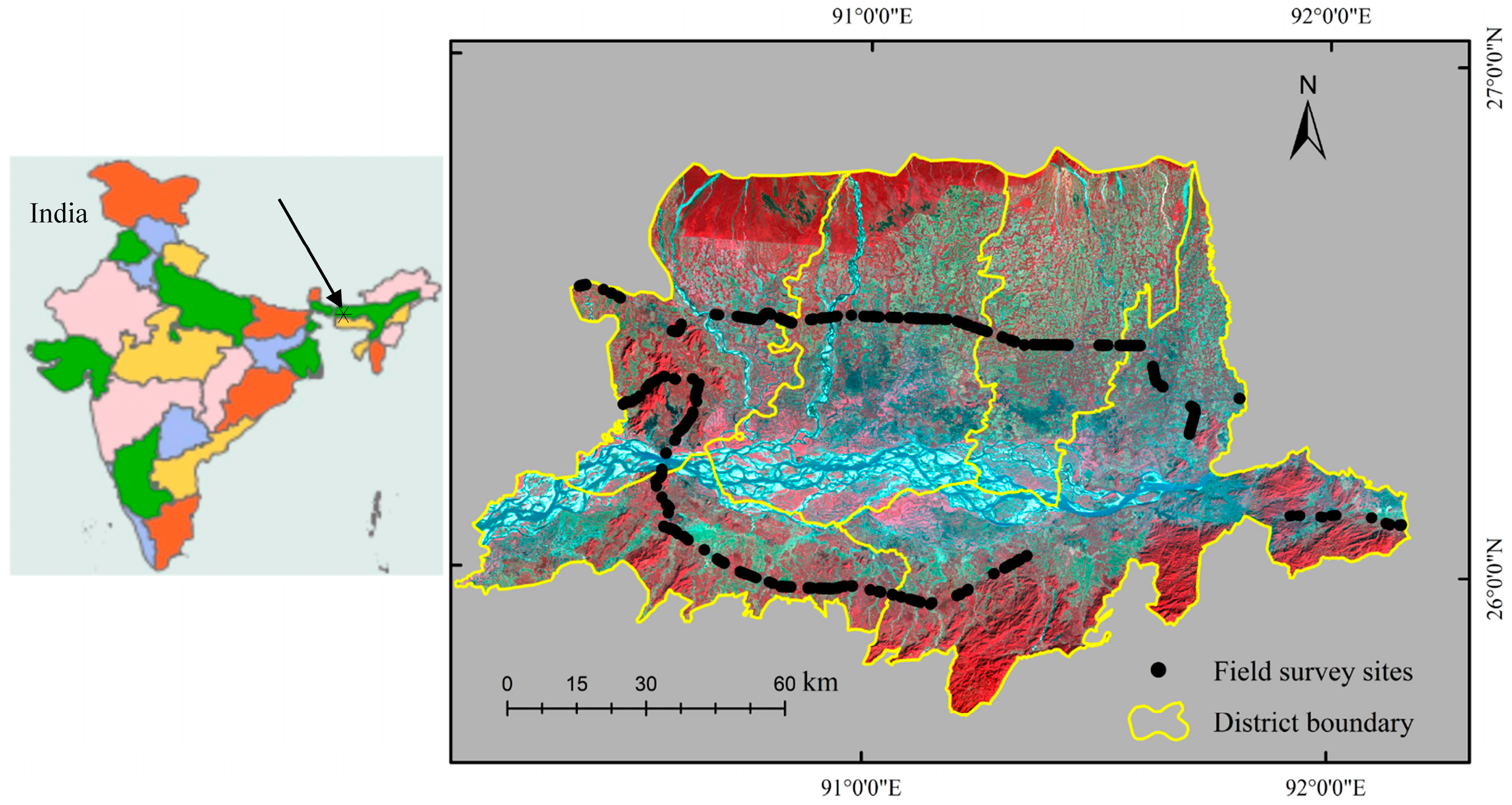
2. Study Area
3. Dataset and Pre-Processing
3.1. MODIS NDVI Data
3.2. HJ-1A/B Data
3.3. Field Data
3.4. Ground Reference Data Generation
3.5. Available Agriculture Statistics Data
4. Methods
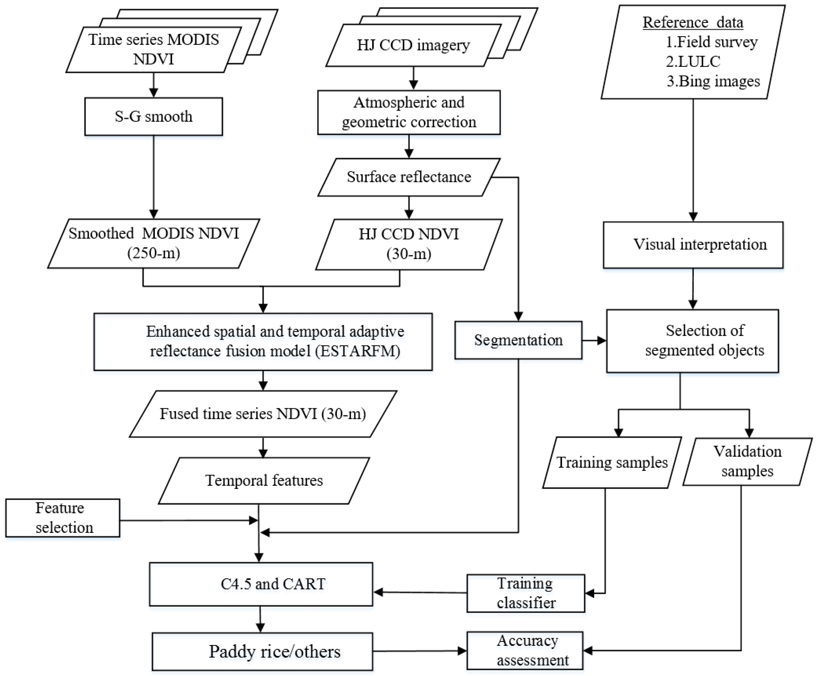
4.1. General Overview of Procedure
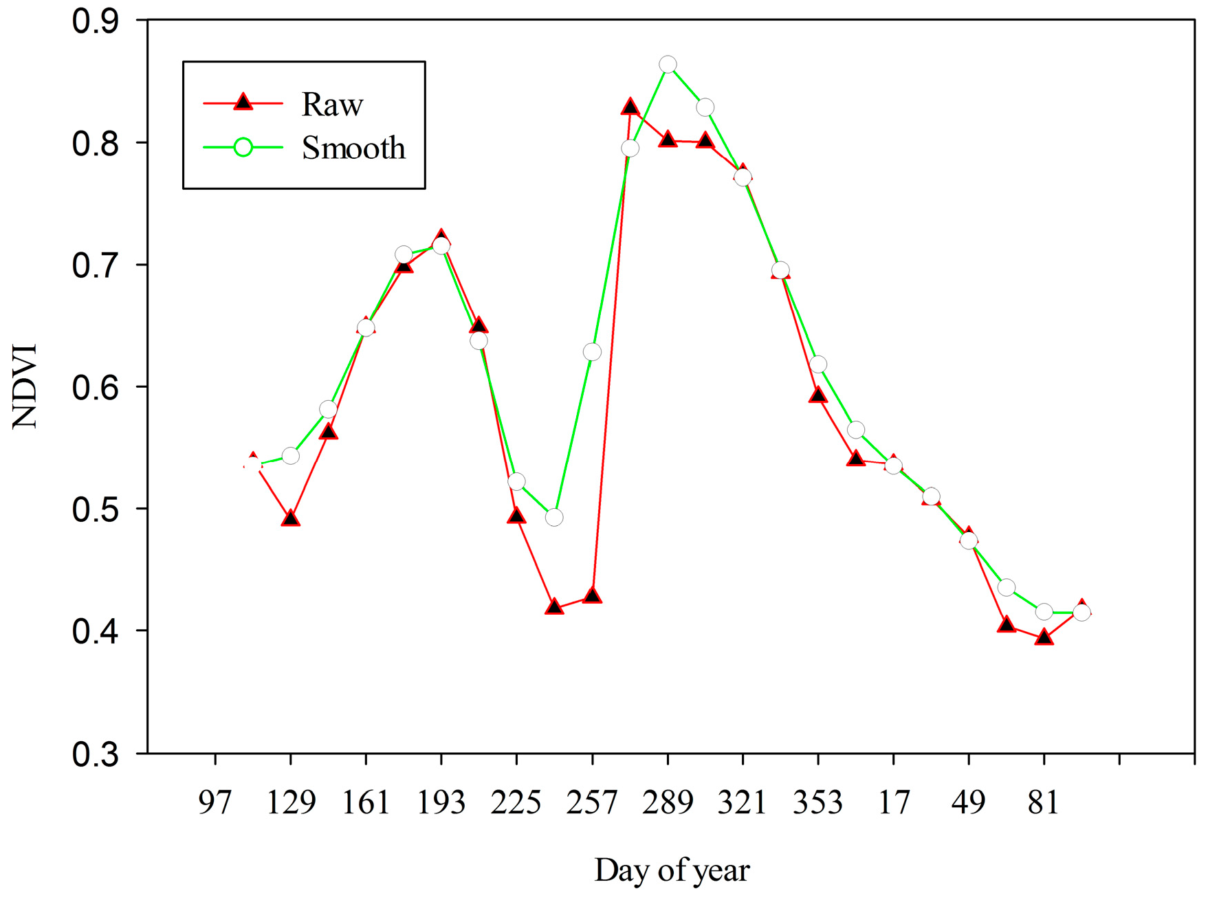
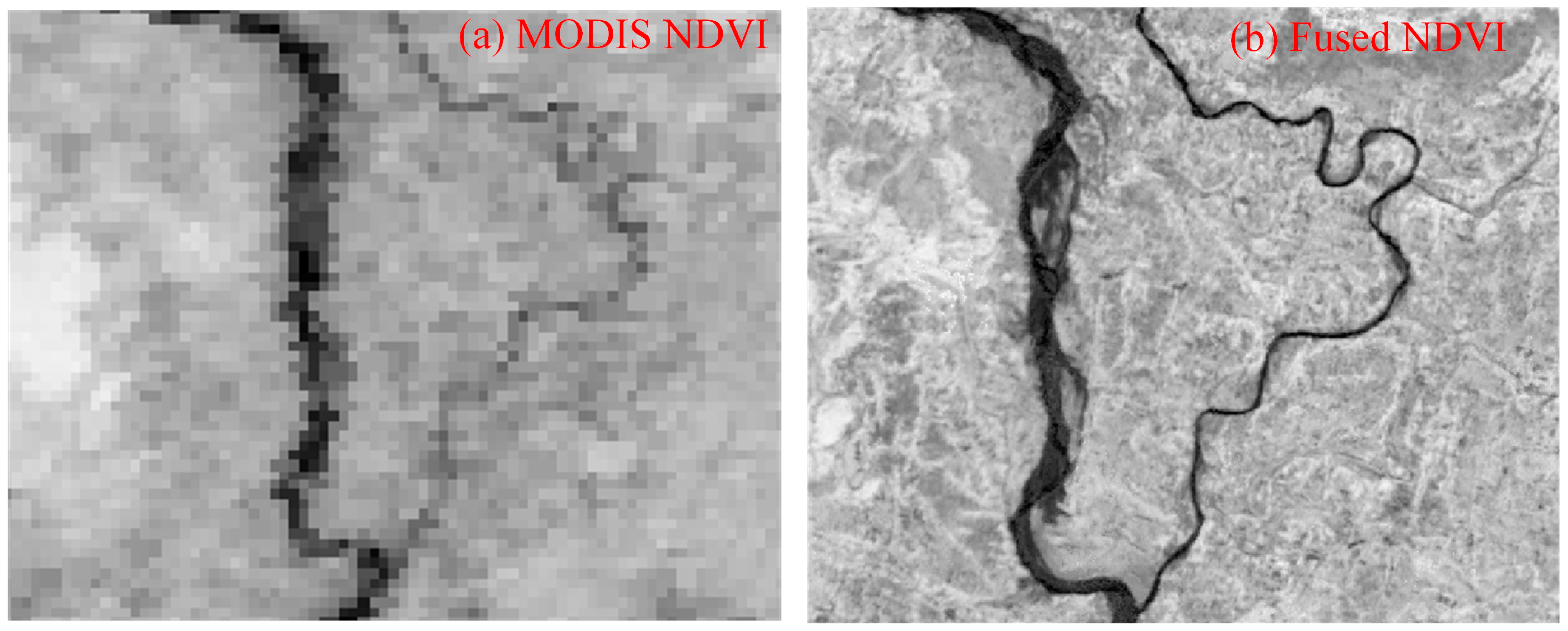
4.2. Fusion of Time Series MODIS NDVI and HJ CCD NDVI
4.3. Temporal Feature Extraction and Ranking
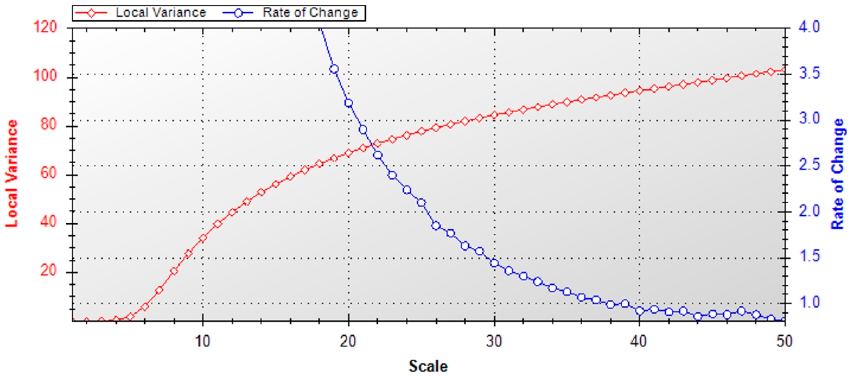
4.4. Image Segmentation for OBIA
4.5. Classification Methods
4.6. Training and Validation Sample Selection
4.7. Accuracy Assessment
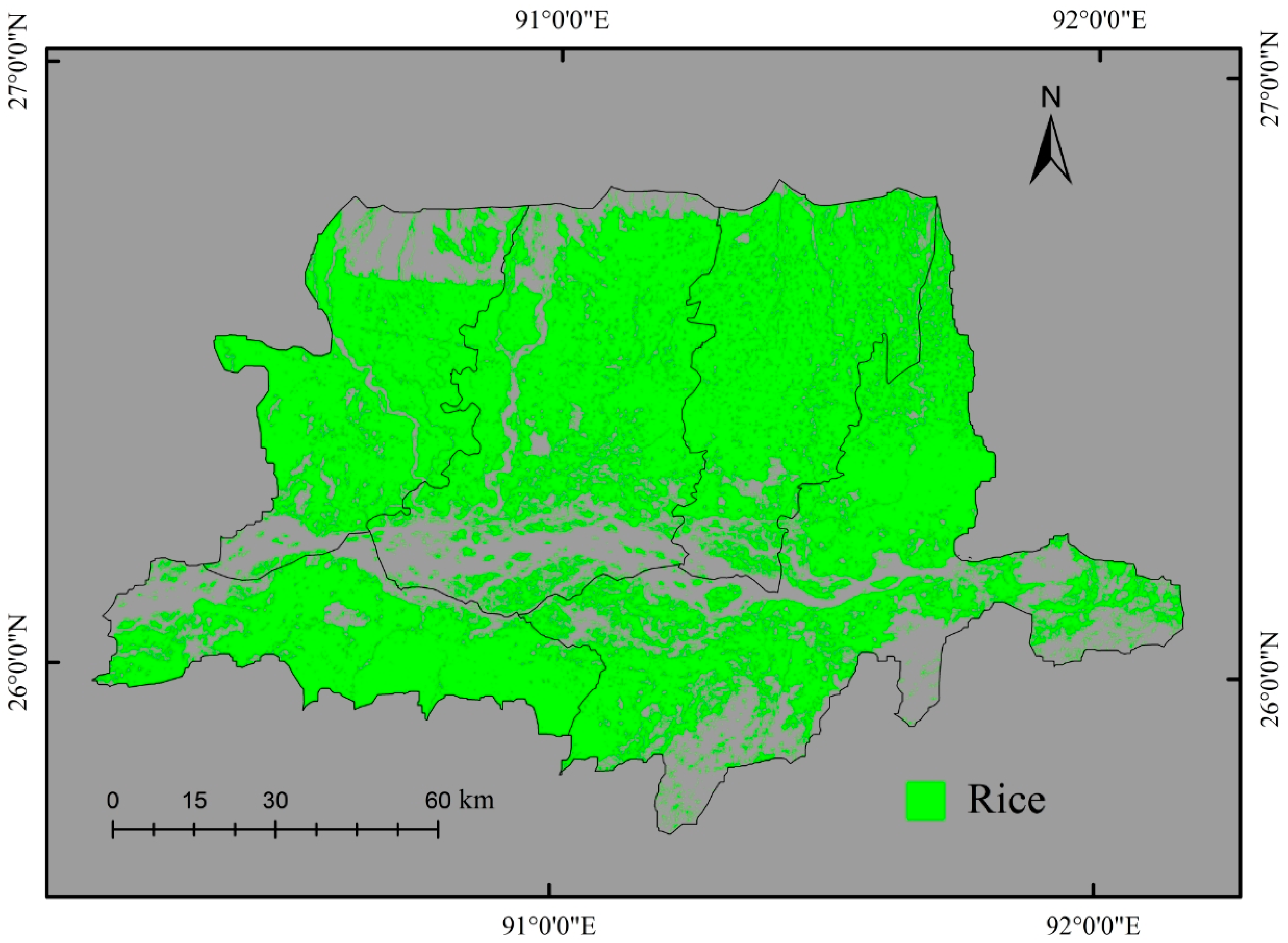
5. Results
5.1. Temporal Feature Analysis and Selection
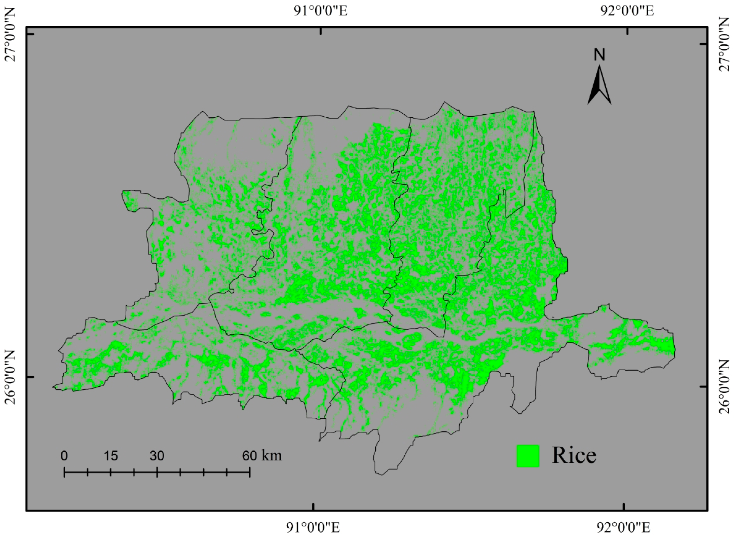
5.2. Classification Results of the Proposed and the Traditional Approaches
5.3. Classification Accuracies
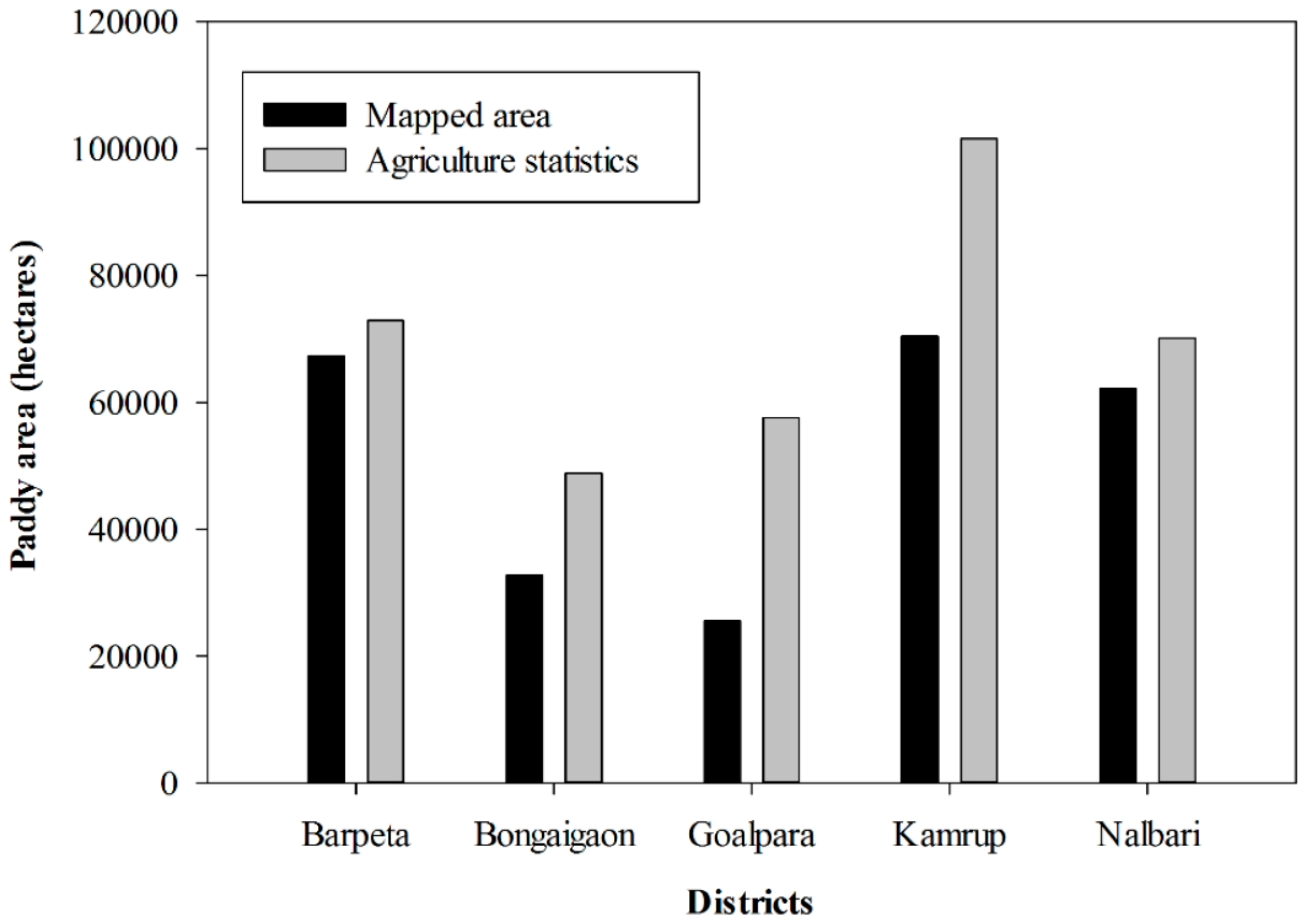
5.4. Comparison to Available Agriculture Statistics Data
6. Discussion
7. Conclusions
Acknowledgments
Author Contributions
Conflicts of Interest
References
- Maclean, J.; Hardy, B.; Hettel, G. Rice Almanac: Source Book for One of the Most Important Economic Activities on Earth; International Rice Research Institute: Los Baños, Philippines, 2013. [Google Scholar]
- Elert, E. Rice by the numbers: A good grain. Nature 2014, 514, 50. [Google Scholar] [CrossRef]
- Bouman, B.A.M.; Humphreys, E.; Tuong, T.P.; Barker, R. Rice and water. Adv. Agron. 2007, 92, 187–237. [Google Scholar]
- Climate Change. Available online: http://ricepedia.org/challenges/climate-change (accessed on 9 December 2016).
- Scheehle, E.; Godwin, D.; Ottinger, D.; DeAngelo, B. Global Anthropogenic Non-CO2 Greenhouse Gas Emissions: 1990–2020; United States Environmental Protection Agency: Washington, DC, USA, 2006.
- Gilbert, M.; Xiao, X.; Pfeiffer, D.U.; Epprecht, M.; Boles, S.; Czarnecki, C.; Chaitaweesub, P.; Kalpravidh, W.; Minh, P.Q.; Otte, M.J. Mapping H5N1 highly pathogenic avian influenza risk in Southeast Asia. Proc. Natl. Acad. Sci. USA 2008, 105, 4769–4774. [Google Scholar] [CrossRef] [PubMed]
- Nguyen, N.V. Global Climate Changes and Rice Food Security; Food and Agriculture Organization: Rome, Italy, 2008. [Google Scholar]
- Chen, J.; Huang, J.; Hu, J. Mapping rice planting areas in southern China using the China Environment Satellite data. Math. Comput. Model. 2011, 54, 1037–1043. [Google Scholar] [CrossRef]
- Fang, H.; Wu, B.; Liu, H.; Huang, X. Using NOAA AVHRR and Landsat TM to estimate rice area year-by-year. Int. J. Remote Sens. 1998, 19, 521–525. [Google Scholar] [CrossRef]
- Gumma, M.K.; Thenkabail, P.S.; Maunahan, A.; Islam, S.; Nelson, A. Mapping seasonal rice cropland extent and area in the high cropping intensity environment of Bangladesh using MODIS 500 m data for the year 2010. ISPRS J. Photogramm. Remote Sens. 2014, 91, 98–113. [Google Scholar] [CrossRef]
- Le Toan, T.; Ribbes, F.; Wang, L.-F.; Floury, N.; Ding, K.-H.; Kong, J.A.; Fujita, M.; Kurosu, T. Rice crop mapping and monitoring using ERS-1 data based on experiment and modeling results. IEEE Trans. Geosci. Remote Sens. 1997, 35, 41–56. [Google Scholar] [CrossRef]
- Rossi, C.; Erten, E. Paddy-rice monitoring using TanDEM-X. IEEE Trans. Geosci. Remote Sens. 2015, 53, 900–910. [Google Scholar] [CrossRef]
- Son, N.-T.; Chen, C.-F.; Chen, C.-R.; Duc, H.-N.; Chang, L.-Y. A phenology-based classification of time-series MODIS data for rice crop monitoring in Mekong Delta, Vietnam. Remote Sens. 2013, 6, 135–156. [Google Scholar] [CrossRef]
- Wang, J.; Huang, J.; Zhang, K.; Li, X.; She, B.; Wei, C.; Gao, J.; Song, X. Rice Fields Mapping in Fragmented Area Using Multi-Temporal HJ-1A/B CCD Images. Remote Sens. 2015, 7, 3467–3488. [Google Scholar] [CrossRef]
- Dong, J.; Xiao, X.; Kou, W.; Qin, Y.; Zhang, G.; Li, L.; Jin, C.; Zhou, Y.; Wang, J.; Biradar, C. Tracking the dynamics of paddy rice planting area in 1986–2010 through time series Landsat images and phenology-based algorithms. Remote Sens. Environ. 2015, 160, 99–113. [Google Scholar] [CrossRef]
- Kontgis, C.; Schneider, A.; Ozdogan, M. Mapping rice paddy extent and intensification in the Vietnamese Mekong river delta with dense time stacks of Landsat data. Remote Sens. Environ. 2015, 169, 255–269. [Google Scholar] [CrossRef]
- Wan, S.; Lei, T.C.; Chou, T.-Y. An enhanced supervised spatial decision support system of image classification: Consideration on the ancillary information of paddy rice area. Int. J. Geogr. Inf. Sci. 2010, 24, 623–642. [Google Scholar] [CrossRef]
- Chen, C.F.; Chen, C.R.; Son, N.T.; Chang, L.Y. Delineating rice cropping activities from MODIS data using wavelet transform and artificial neural networks in the Lower Mekong countries. Agric. Ecosyst. Environ. 2012, 162, 127–137. [Google Scholar] [CrossRef]
- Xiao, X.; Boles, S.; Frolking, S.; Li, C.; Babu, J.Y.; Salas, W.; Moore, B. Mapping paddy rice agriculture in South and Southeast Asia using multi-temporal MODIS images. Remote Sens. Environ. 2006, 100, 95–113. [Google Scholar] [CrossRef]
- Gumma, M.K.; Nelson, A.; Thenkabail, P.S.; Singh, A.N. Mapping rice areas of South Asia using MODIS multitemporal data. J. Appl. Remote Sens. 2011, 5, 053547. [Google Scholar] [CrossRef]
- Bridhikitti, A.; Overcamp, T.J. Estimation of Southeast Asian rice paddy areas with different ecosystems from moderate-resolution satellite imagery. Agric. Ecosyst. Environ. 2012, 146, 113–120. [Google Scholar] [CrossRef]
- Singha, M.; Wu, B.; Zhang, M. An Object-Based Paddy Rice Classification Using Multi-Spectral Data and Crop Phenology in Assam, Northeast India. Remote Sens. 2016, 8, 479. [Google Scholar] [CrossRef]
- Dong, J.; Xiao, X.; Menarguez, M.A.; Zhang, G.; Qin, Y.; Thau, D.; Biradar, C.; Moore, B. Mapping paddy rice planting area in northeastern Asia with Landsat 8 images, phenology-based algorithm and Google Earth Engine. Remote Sens. Environ. 2016, 185, 142–154. [Google Scholar] [CrossRef]
- Wang, J.; Xiao, X.; Qin, Y.; Dong, J.; Zhang, G.; Kou, W.; Jin, C.; Zhou, Y.; Zhang, Y. Mapping paddy rice planting area in wheat-rice double-cropped areas through integration of Landsat-8 OLI, MODIS, and PALSAR images. Sci. Rep. 2015, 5, 10088. [Google Scholar] [CrossRef] [PubMed]
- Simonneaux, V.; Duchemin, B.; Helson, D.; Er-Raki, S.; Olioso, A.; Chehbouni, A.G. The use of high-resolution image time series for crop classification and evapotranspiration estimate over an irrigated area in central Morocco. Int. J. Remote Sens. 2008, 29, 95–116. [Google Scholar] [CrossRef] [Green Version]
- Blaschke, T. Object based image analysis for remote sensing. ISPRS J. Photogramm. Remote Sens. 2010, 65, 2–16. [Google Scholar] [CrossRef]
- Definiens, A.G. Definiens eCognition Developer 8 Reference Book; Definiens: Munich, Germany, 2009. [Google Scholar]
- Blaschke, T.; Hay, G.J.; Kelly, M.; Lang, S.; Hofmann, P.; Addink, E.; Feitosa, R.Q.; van der Meer, F.; van der Werff, H.; van Coillie, F. Geographic object-based image analysis—Towards a new paradigm. ISPRS J. Photogramm. Remote Sens. 2014, 87, 180–191. [Google Scholar] [CrossRef] [PubMed]
- Johansen, K.; Arroyo, L.A.; Phinn, S.; Witte, C. Comparison of geo-object based and pixel-based change detection of riparian environments using high spatial resolution multi-spectral imagery. Photogramm. Eng. Remote Sens. 2010, 76, 123–136. [Google Scholar] [CrossRef]
- Qiu, B.; Li, W.; Tang, Z.; Chen, C.; Qi, W. Mapping paddy rice areas based on vegetation phenology and surface moisture conditions. Ecol. Indic. 2015, 56, 79–86. [Google Scholar] [CrossRef]
- Xiao, X.; Boles, S.; Liu, J.; Zhuang, D.; Frolking, S.; Li, C.; Salas, W.; Moore, B. Mapping paddy rice agriculture in southern China using multi-temporal MODIS images. Remote Sens. Environ. 2005, 95, 480–492. [Google Scholar] [CrossRef]
- Gao, F.; Masek, J.; Schwaller, M.; Hall, F. On the blending of the Landsat and MODIS surface reflectance: Predicting daily Landsat surface reflectance. IEEE Trans. Geosci. Remote Sens. 2006, 44, 2207–2218. [Google Scholar]
- Zhu, X.; Chen, J.; Gao, F.; Chen, X.; Masek, J.G. An enhanced spatial and temporal adaptive reflectance fusion model for complex heterogeneous regions. Remote Sens. Environ. 2010, 114, 2610–2623. [Google Scholar] [CrossRef]
- Schmidt, M.; Udelhoven, T.; Gill, T.; Röder, A. Long term data fusion for a dense time series analysis with MODIS and Landsat imagery in an Australian Savanna. J. Appl. Remote Sens. 2012, 6, 063512. [Google Scholar]
- Li, Q.; Wang, C.; Zhang, B.; Lu, L. Object-Based Crop Classification with Landsat-MODIS Enhanced Time-Series Data. Remote Sens. 2015, 7, 16091–16107. [Google Scholar] [CrossRef]
- Ahmed, T.; Chetia, S.K.; Chowdhury, R.; Ali, S. Status Paper on Rice in Assam: Rice Knowledge Management Portal; Directorate of Rice Research: Telangana, India, 2011. [Google Scholar]
- LP DAAC: NASA Land Data Products and Services. Data Pool. Available online: https://lpdaac.usgs.gov/data_access/data_pool (accessed on 1 March 2016).
- Chen, J.; Jönsson, P.; Tamura, M.; Gu, Z.; Matsushita, B.; Eklundh, L. A simple method for reconstructing a high-quality NDVI time-series data set based on the Savitzky–Golay filter. Remote Sens. Environ. 2004, 91, 332–344. [Google Scholar] [CrossRef]
- Leinenkugel, P.; Kuenzer, C.; Oppelt, N.; Dech, S. Characterisation of land surface phenology and land cover based on moderate resolution satellite data in cloud prone areas—A novel product for the Mekong Basin. Remote Sens. Environ. 2013, 136, 180–198. [Google Scholar] [CrossRef]
- China Resources Satellite Application Center. Available online: http://cresda.com.cn/EN/ (accessed on 1 March 2016).
- Zhu, X.; Gao, F.; Liu, D.; Chen, J. A modified neighborhood similar pixel interpolator approach for removing thick clouds in Landsat images. IEEE Geosci. Remote Sens. Lett. 2012, 9, 521–525. [Google Scholar] [CrossRef]
- Bing Maps. Available online: https://www.bing.com/maps/ (accessed on 21 December 2016).
- Wu, B.; Li, Q. Crop planting and type proportion method for crop acreage estimation of complex agricultural landscapes. Int. J. Appl. Earth Obs. Geoinf. 2012, 16, 101–112. [Google Scholar] [CrossRef]
- Xiao, X.; Dorovskoy, P.; Biradar, C.; Bridge, E. A library of georeferenced photos from the field. Eos Trans. Am. Geophys. Union 2011, 92, 453–454. [Google Scholar] [CrossRef]
- Gateway to Indian Earth Observation. Available online: http://bhuvan.nrsc.gov.in/bhuvan_links.php (accessed on 1 March 2016).
- Welcome to the QGIS project! Available online: http://qgis.org/en/site/ (accessed on 1 March 2016).
- Directorate of Economics and Statistics, Assam. Available online: http://ecostatassam.nic.in/ (accessed on 1 March 2016).
- Breiman, L.; Friedman, J.; Stone, C.J.; Olshen, R.A. Classification and Regression Trees; CRC Press: Boca Raton, FL, USA, 1984. [Google Scholar]
- Quinlan, J.R. C4.5: Programs for Machine Learning, 1st ed.; Morgan Kaufmann Series Machine Learning; Morgan Kaufmann Publishers: Burlington, MA, USA, 1993. [Google Scholar]
- Tian, F.; Wang, Y.; Fensholt, R.; Wang, K.; Zhang, L.; Huang, Y. Mapping and evaluation of NDVI trends from synthetic time series obtained by blending Landsat and MODIS data around a coalfield on the Loess Plateau. Remote Sens. 2013, 5, 4255–4279. [Google Scholar] [CrossRef]
- Hwang, T.; Song, C.; Bolstad, P.V.; Band, L.E. Downscaling real-time vegetation dynamics by fusing multi-temporal MODIS and Landsat NDVI in topographically complex terrain. Remote Sens. Environ. 2011, 115, 2499–2512. [Google Scholar] [CrossRef]
- Olexa, E.M.; Lawrence, R.L. Performance and effects of land cover type on synthetic surface reflectance data and NDVI estimates for assessment and monitoring of semi-arid rangeland. Int. J. Appl. Earth Obs. Geoinf. 2014, 30, 30–41. [Google Scholar] [CrossRef]
- Walker, J.J.; De Beurs, K.M.; Wynne, R.H.; Gao, F. Evaluation of Landsat and MODIS data fusion products for analysis of dryland forest phenology. Remote Sens. Environ. 2012, 117, 381–393. [Google Scholar] [CrossRef]
- Diao, C.; Wang, L. Incorporating plant phenological trajectory in exotic saltcedar detection with monthly time series of Landsat imagery. Remote Sens. Environ. 2016, 182, 60–71. [Google Scholar] [CrossRef]
- Jonsson, P.; Eklundh, L. Seasonality extraction by function fitting to time-series of satellite sensor data. Geosci. IEEE Trans. Remote Sens. 2002, 40, 1824–1832. [Google Scholar] [CrossRef]
- Robnik-Šikonja, M.; Kononenko, I. Theoretical and empirical analysis of ReliefF and RReliefF. Mach. Learn. 2003, 53, 23–69. [Google Scholar] [CrossRef]
- Baatz, M.; Schäpe, A. Multiresolution segmentation. In Angewandte Geographische Informationsverarbeitung XII; Herbert Wichmann Verlag: Heidelberg, Germany, 2000; pp. 12–23. [Google Scholar]
- Drӑguţ, L.; Tiede, D.; Levick, S.R. ESP: A tool to estimate scale parameter for multiresolution image segmentation of remotely sensed data. Int. J. Geogr. Inf. Sci. 2010, 24, 859–871. [Google Scholar] [CrossRef]
- Vieira, M.A.; Formaggio, A.R.; Rennó, C.D.; Atzberger, C.; Aguiar, D.A.; Mello, M.P. Object based image analysis and data mining applied to a remotely sensed Landsat time-series to map sugarcane over large areas. Remote Sens. Environ. 2012, 123, 553–562. [Google Scholar] [CrossRef]
- Hall, M.; Frank, E.; Holmes, G.; Pfahringer, B.; Reutemann, P.; Witten, I.H. The WEKA data mining software: An update. ACM SIGKDD Explor. Newsl. 2009, 11, 10–18. [Google Scholar] [CrossRef]
- Lawrence, R.L.; Wright, A. Rule-based classification systems using classification and regression tree (CART) analysis. Photogramm. Eng. Remote Sens. 2001, 67, 1137–1142. [Google Scholar]
- Shao, Y.; Lunetta, R.S. Comparison of support vector machine, neural network, and CART algorithms for the land-cover classification using limited training data points. ISPRS J. Photogramm. Remote Sens. 2012, 70, 78–87. [Google Scholar] [CrossRef]
- Congalton, R.G.; Green, K. Assessing the Accuracy of Remotely Sensed Data: Principles and Practices; CRC Press: Boca Raton, FL, USA, 2008. [Google Scholar]
- Peña, J.M.; Gutiérrez, P.A.; Hervás-Martínez, C.; Six, J.; Plant, R.E.; López-Granados, F. Object-based image classification of summer crops with machine learning methods. Remote Sens. 2014, 6, 5019–5041. [Google Scholar] [CrossRef]
- Gutiérrez, P.A.; Hervás-Martínez, C.; Martínez-Estudillo, F.J.; Carbonero, M. A two-stage evolutionary algorithm based on sensitivity and accuracy for multi-class problems. Inf. Sci. 2012, 197, 20–37. [Google Scholar] [CrossRef]
- Karkee, M.; Steward, B.L.; Tang, L.; Aziz, S.A. Quantifying sub-pixel signature of paddy rice field using an artificial neural network. Comput. Electron. Agric. 2009, 65, 65–76. [Google Scholar] [CrossRef]
- Peña-Barragán, J.M.; Ngugi, M.K.; Plant, R.E.; Six, J. Object-based crop identification using multiple vegetation indices, textural features and crop phenology. Remote Sens. Environ. 2011, 115, 1301–1316. [Google Scholar] [CrossRef]
- Kim, H.-O.; Yeom, J.-M. Effect of red-edge and texture features for object-based paddy rice crop classification using RapidEye multi-spectral satellite image data. Int. J. Remote Sens. 2014, 35, 7046–7068. [Google Scholar] [CrossRef]
- Li, Q.; Cao, X.; Jia, K.; Zhang, M.; Dong, Q. Crop type identification by integration of high-spatial resolution multispectral data with features extracted from coarse-resolution time-series vegetation index data. Int. J. Remote Sens. 2014, 35, 6076–6088. [Google Scholar] [CrossRef]
- Manjunatha, A.V.; Anik, A.R.; Speelman, S.; Nuppenau, E.A. Impact of land fragmentation, farm size, land ownership and crop diversity on profit and efficiency of irrigated farms in India. Land Use Policy 2013, 31, 397–405. [Google Scholar] [CrossRef]
- Goverment of India, Ministry of Agriculture. Department of Agriculture and Cooperation Agricultural Statistics at a Glance 2014; Govermant of India, Ministry of Agriculture: Haryana, India, 2015.
- Zhu, Z.; Woodcock, C.E.; Holden, C.; Yang, Z. Generating synthetic Landsat images based on all available Landsat data: Predicting Landsat surface reflectance at any given time. Remote Sens. Environ. 2015, 162, 67–83. [Google Scholar] [CrossRef]
- Asner, G.P. Cloud cover in Landsat observations of the Brazilian Amazon. Int. J. Remote Sens. 2001, 22, 3855–3862. [Google Scholar] [CrossRef]
- Jarihani, A.A.; McVicar, T.R.; Van Niel, T.G.; Emelyanova, I.V.; Callow, J.N.; Johansen, K. Blending Landsat and MODIS data to generate multispectral indices: A comparison of “Index-then-Blend” and “Blend-then-Index” approaches. Remote Sens. 2014, 6, 9213–9238. [Google Scholar] [CrossRef] [Green Version]
- Nguyen, T.T.H.; De Bie, C.; Ali, A.; Smaling, E.M.A.; Chu, T.H. Mapping the irrigated rice cropping patterns of the Mekong delta, Vietnam, through hyper-temporal SPOT NDVI image analysis. Int. J. Remote Sens. 2012, 33, 415–434. [Google Scholar] [CrossRef]
- Oguro, Y.; Suga, Y.; Takeuchi, S.; Ogawa, M.; Konishi, T.; Tsuchiya, K. Comparison of SAR and optical sensor data for monitoring of rice plant around Hiroshima. Adv. Space Res. 2001, 28, 195–200. [Google Scholar] [CrossRef]
- Shiu, Y.-S.; Lin, M.-L.; Huang, C.-H.; Chu, T.-H. Mapping paddy rice agriculture in a highly fragmented area using a geographic information system object-based post classification process. J. Appl. Remote Sens. 2012, 6, 063526. [Google Scholar]


| Satellite | Sensor | Acquisition Time (dd-mm-yyyy) | Paddy Rice Phenology Stage |
|---|---|---|---|
| HJ-1A | CCD2 | 22-10-2014 | Heading |
| HJ-1A | CCD1 | 05-12-2014 | Ripening |
| HJ-1B | CCD1 | 09-03-2015 | Planting |
| MODIS | Terra | 07-04-2014 to 22-03-2015 | Sowing–Harvesting |
| Satellite | Sensor | Bands | Spectral Range ( | Spatial Resolution (m) | Swath Width (km) | Revisit Period (day) |
|---|---|---|---|---|---|---|
| HJ-1 A/B | CCD | 1 | 0.43–0.52 | 30 | 360 | 4 |
| 2 | 0.52–0.60 | |||||
| 3 | 0.63–0.69 | |||||
| 4 | 0.76–0.90 |
| Features | Definition | Relations to Vegetation |
|---|---|---|
| Maximum value | The largest NDVI value of the time series | Seasonal highest greenness value |
| Minimum value | The smallest NDVI value of the time series | Seasonal lowest greenness value |
| Mean value | The mean NDVI value of the time series | Mean greenness level |
| Standard deviation value | The standard deviation value of NDVI time series | Standard deviation of greenness level |
| Base NDVI value (BV) | The average of the left and right minimum value of fitted function | Soil background conditions |
| Amplitude (Amp) | The difference between the maximum and the base NDVI value | Seasonal range of greenness variation |
| Left derivative (LD) | The ratio of the difference between the left 20% and 80% levels to the corresponding time difference | Rate of greening and vegetation growth |
| Right derivative (RD) | The ratio of the difference between the right 20% and 80% levels to the corresponding time difference | Rate of browning and senescence |
| Large seasonal integral (LI) | The sum of the representative function with a positive fit during the growing season | Vegetation production over the growing season |
| Small seasonal integral (SI) | The sum of the difference between the fitted function and the base level during the growing season | Seasonally active vegetation production over the growing season |
| 23 NDVI layers | Fused time series NDVI of one year | Seasonal variation of greenness over a year |
| No. | Features | Rank |
|---|---|---|
| 1 | Standard Deviation value | 0.09315 |
| 2 | NDVI-2015017 | 0.08965 |
| 3 | NDVI-2015065 | 0.08347 |
| 4 | NDVI-2014113 | 0.07607 |
| 5 | NDVI-2014193 | 0.07595 |
| 6 | NDVI-2014337 | 0.07456 |
| 7 | NDVI-2014257 | 0.07451 |
| 8 | LI | 0.07302 |
| 9 | Minimum value | 0.07166 |
| 10 | NDVI-2015001 | 0.07054 |
| 11 | NDVI-2015081 | 0.07015 |
| 12 | Mean value | 0.07004 |
| 13 | NDVI-2014209 | 0.07003 |
| 14 | Maximum value | 0.06843 |
| 15 | NDVI-2014225 | 0.06827 |
| Strategy | C4.5 | CART | ||||
|---|---|---|---|---|---|---|
| CCR (%) | Kappa Coefficient | Paddy Rice MS (%) | CCR (%) | Kappa Coefficient | Paddy Rice MS (%) | |
| Single-date spectral image of October (OI) | 65.62 | 0.33 | 57.70 | 56.25 | 0.14 | 52.40 |
| OI+ all temporal features | 81.25 | 0.61 | 90.90 | 81.25 | 0.61 | 90.90 |
| OI+ best-selected temporal features | 84.37 | 0.68 | 81.30 | 87.50 | 0.75 | 82.40 |
| Temporal spectral images | 90.62 | 0.81 | 87.50 | 78.12 | 0.55 | 78.60 |
| Districts | Derived Paddy Area (2014–2015) | Agriculture Statistics (2012–2013) |
|---|---|---|
| (Thousand Hectares) | (Thousand Hectares) | |
| Barpeta | 70.83 | 72.94 |
| Bongaigaon | 39.50 | 48.85 |
| Goalpara | 41.91 | 57.61 |
| Kamrup | 96.70 | 101.52 |
| Nalbari | 69.16 | 70.13 |
| Total | 318.10 | 351.05 |
© 2016 by the authors; licensee MDPI, Basel, Switzerland. This article is an open access article distributed under the terms and conditions of the Creative Commons Attribution (CC-BY) license (http://creativecommons.org/licenses/by/4.0/).
Share and Cite
Singha, M.; Wu, B.; Zhang, M. Object-Based Paddy Rice Mapping Using HJ-1A/B Data and Temporal Features Extracted from Time Series MODIS NDVI Data. Sensors 2017, 17, 10. https://doi.org/10.3390/s17010010
Singha M, Wu B, Zhang M. Object-Based Paddy Rice Mapping Using HJ-1A/B Data and Temporal Features Extracted from Time Series MODIS NDVI Data. Sensors. 2017; 17(1):10. https://doi.org/10.3390/s17010010
Chicago/Turabian StyleSingha, Mrinal, Bingfang Wu, and Miao Zhang. 2017. "Object-Based Paddy Rice Mapping Using HJ-1A/B Data and Temporal Features Extracted from Time Series MODIS NDVI Data" Sensors 17, no. 1: 10. https://doi.org/10.3390/s17010010