
Quantitative Inspection of Remanence of Broken Wire Rope Based on Compressed Sensing

Abstract
:1. Introduction
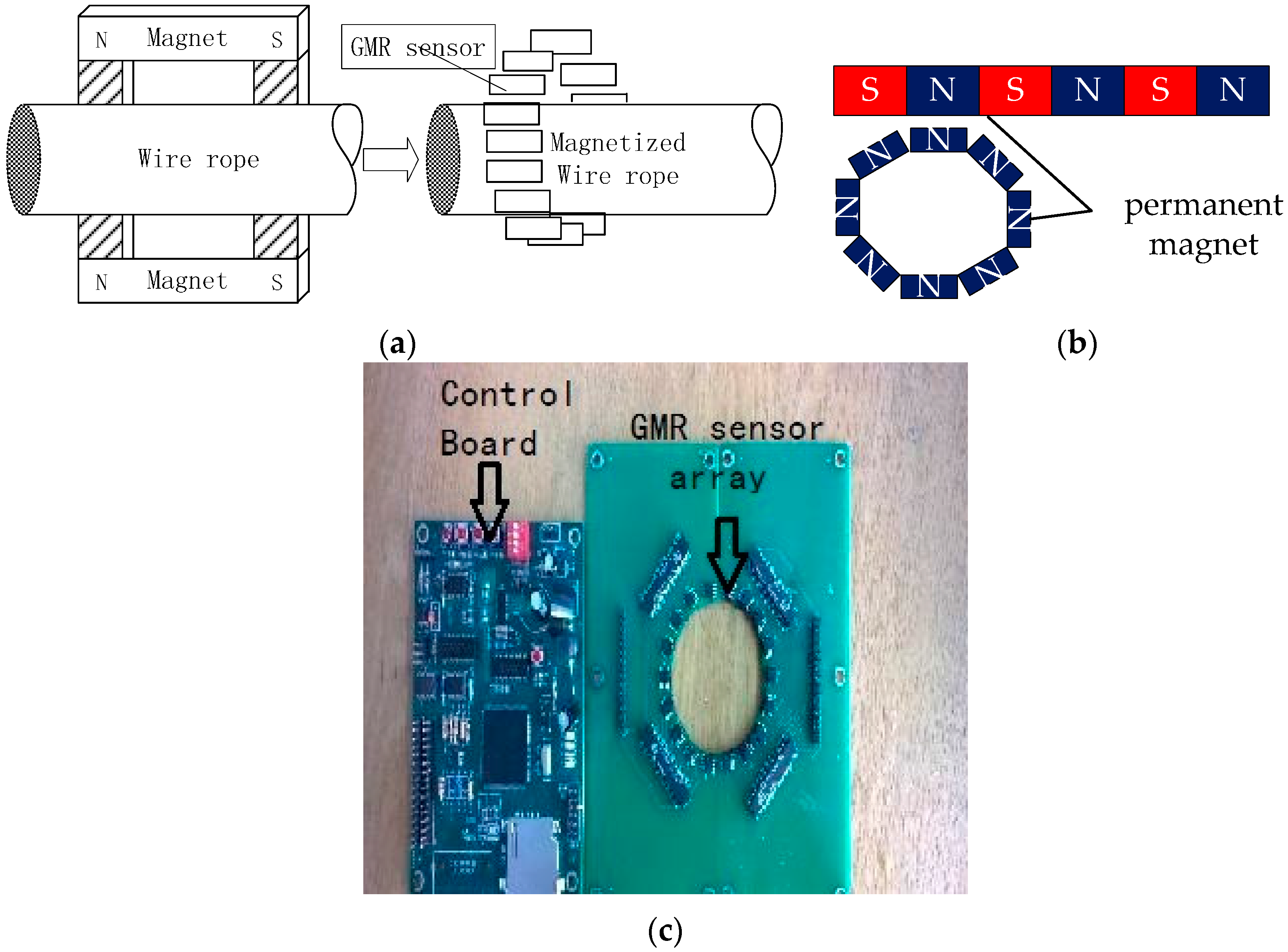
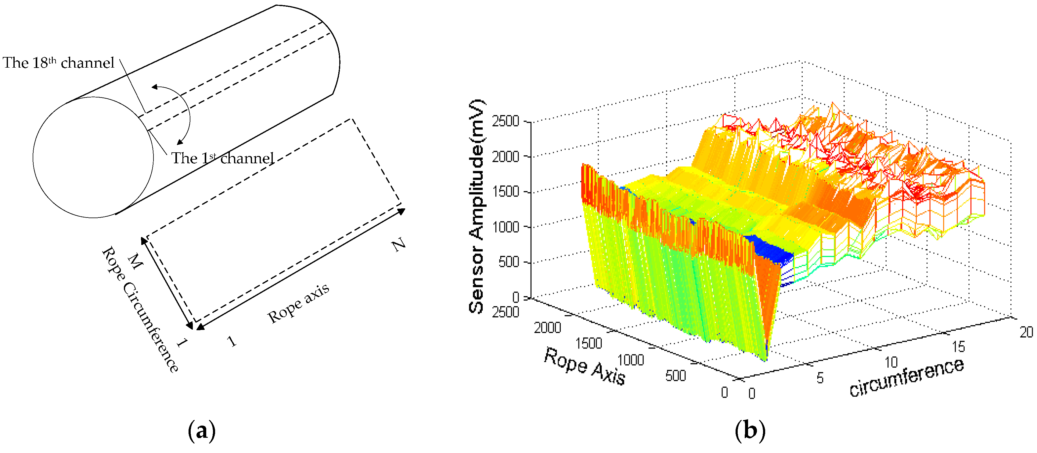
2. Acquiring MFL Signal of Remanence
3. Data Processing
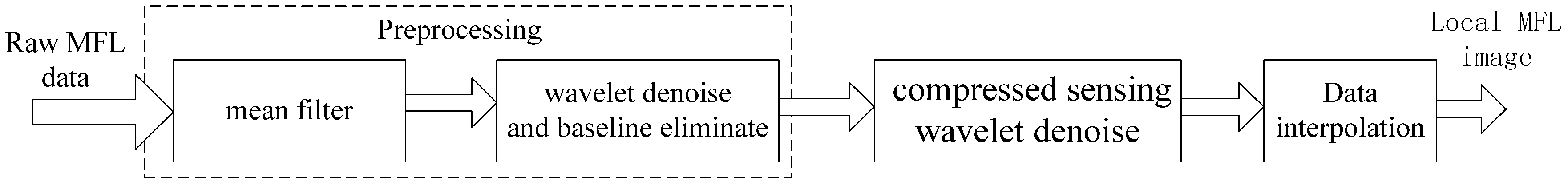
3.1. Signal Pre-Processing
3.2. Denoising Based on CSWF
- (1)
- For the pre-processed signal , the Mallat decomposition algorithm is used and the wavelet coefficients Wj under each scale j are obtained.
- (2)
- The appropriate random measurement matrix (here is a 350 × 1024 Gaussian matrix), is selected, and the wavelet coefficients of linear measurements y under the measurement matrix are calculated.
- (3)
- Through the OMP algorithm, the most-sparse wavelet coefficient is reconstructed; the algorithm steps are as follows:Step One: residue, , and index set, (empty set), are initializedFor iteration, t is 1 to K (K is the sparse degree; here it is 8.)BeginStep Two: the inner product is calculatedThen, the column of whose inner product is the maximum in is obtained: ;The subscript is stored, and the most orthogonal column of Φ: , the selected column of , is set to 0;Step Three: The least-squares method is used ;Step Four: Approximation is updated;The residue, , is updated;End
- (4)
- Using approximate wavelet coefficients the MFL signals are reestablished.
3.3. MFL Image Processing
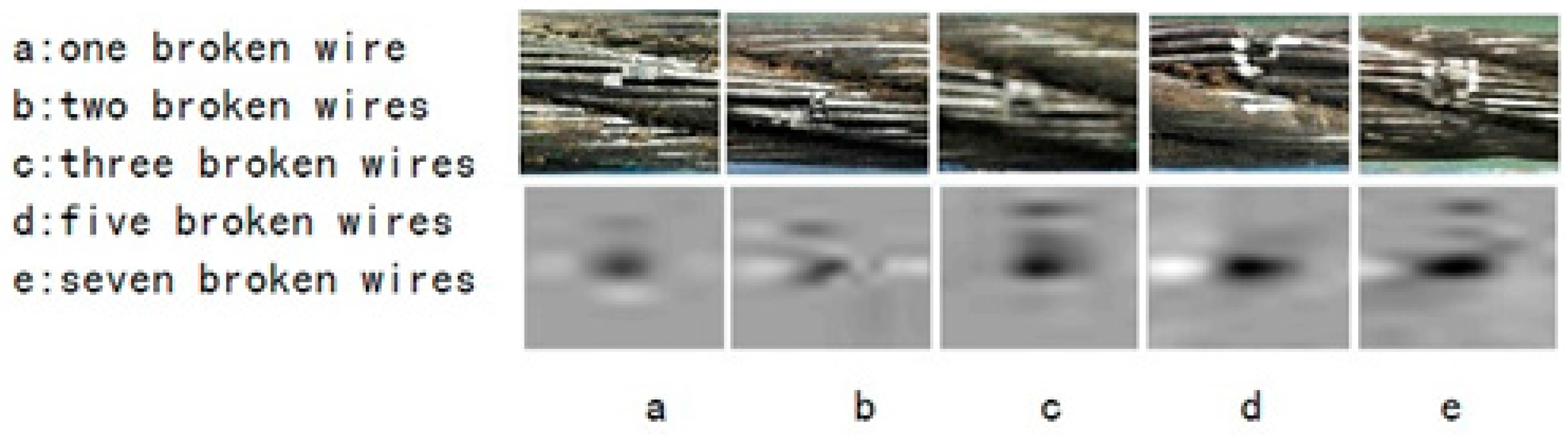
3.3.1. Defect Image Extraction
3.3.2. Defect Characteristic Exactions
- 1.
- Basic Description of Image Shape
- 2.
- Characteristic Descriptions of Shape
- 3.
- Characteristics of Invariant Moment
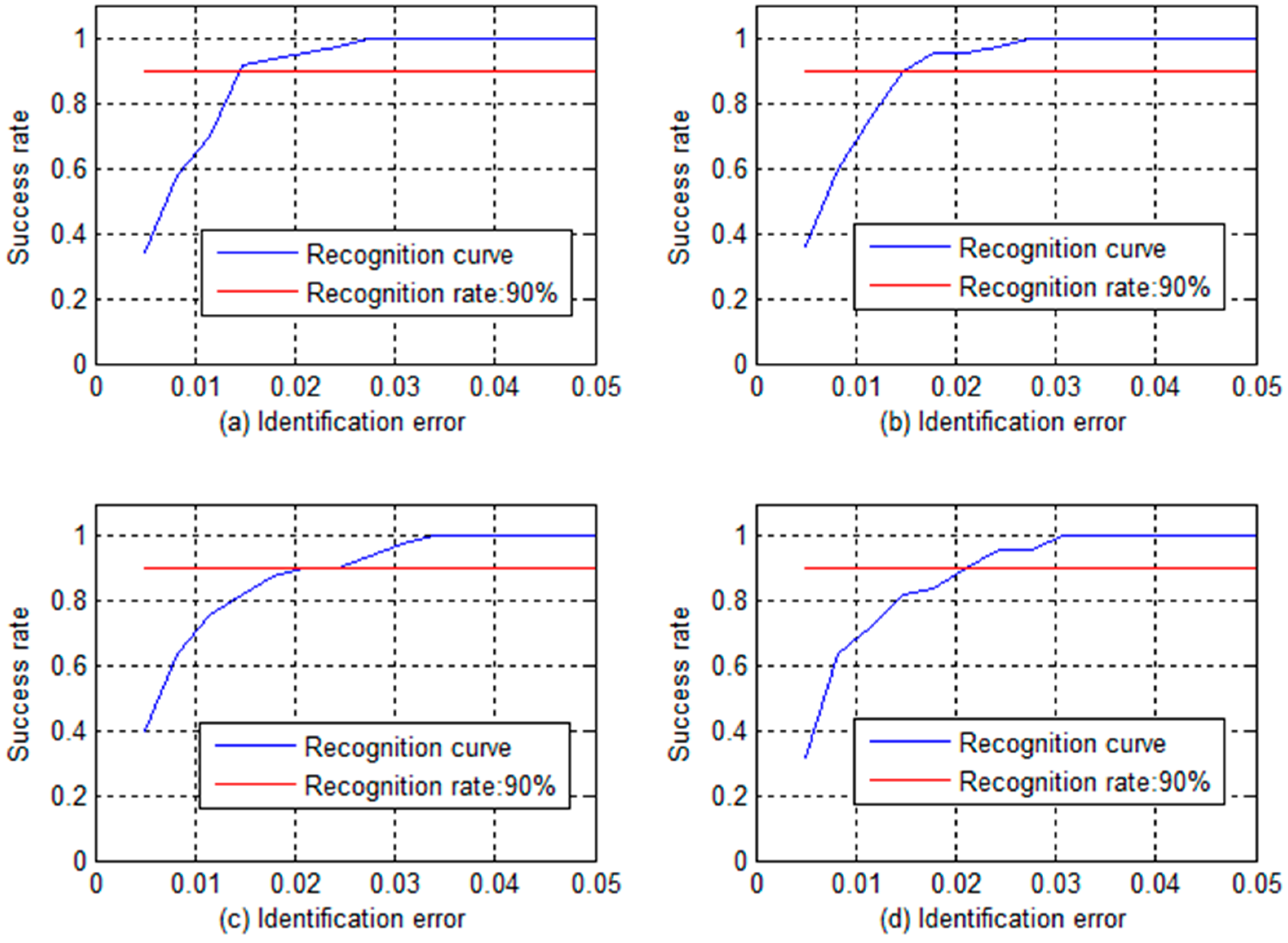
4. Quantitative Recognition
5. Comment and Discussion
6. Conclusions
Acknowledgments
Author Contributions
Conflicts of Interest
References
- Cao, Y.N.; Zhang, D.L.; Xu, D.G. The State-of-Art of Quantitative Testing of Wire Rope. Nondestruct. Test. 2005, 27, 91–95. (In Chinese) [Google Scholar]
- Jomdecha, C.; Prateepasen, A. Design of modified electromagnetic main-flux for steel wire rope inspection. NDT E Int. 2009, 42, 77–83. [Google Scholar] [CrossRef]
- Cao, Q.S.; Liu, D.; Zhou, J.H.; Zhou, J.M. Non-destructive and quantitative detection method for broken wire rope. Chin. J. Sci. Instrum. 2011, 32, 787–794. [Google Scholar]
- Kreak, J.; Peterka, P.; Kropuch, S.; Novak, L. Measurement of tight in steel ropes by a mean of thermovision. Meas. J. Int. Meas. Confed. 2014, 50, 93–98. [Google Scholar] [CrossRef]
- Peng, P.C.; Wang, C.Y. Use of gamma rays in the inspection of steel wire ropes in suspension bridges. NDT E Int. 2015, 75, 80–86. [Google Scholar] [CrossRef]
- Li, X.G.; Miao, C.Y.; Zhang, Y.; Wang, W. Automatic fault detection for steel cord conveyor belt based on statistical features. J. China Coal Soc. 2012, 37, 1233–1238. [Google Scholar]
- Wang, H.Y.; Tian, J. Method of magnetic collect detection for coal mine wire rope base on finite element analysis. J. China Coal Soc. 2013, 38, 256–260. [Google Scholar]
- Wang, H.Y.; Xu, Z.; Hua, G.; Tian, J.; Zhou, B.B.; Lu, Y.H.; Chen, F.J. Key technique of a detection sensor for coal mine wire ropes. Min. Sci. Technol. 2009, 19, 170–175. [Google Scholar] [CrossRef]
- Li, W.; Feng, W.; Li, Z.; Yan, C. Dimension design of excitation structure for wire rope nondestructive testing. J. Tongji Univ. 2012, 40, 1888–1893. [Google Scholar]
- Cao, Y.N.; Zhang, D.L.; Xu, D.G. Study on algorithms of wire rope localized flaw quantitative analysis based on three-dimensional magnetic flux leakage. Acta Electron. Sin. 2007, 35, 1170–1173. [Google Scholar]
- Zhang, D.L.; Zhao, M.; Zhou, Z.H. Quantitative Inspection of Wire Rope Discontinuities using Magnetic Flux Leakage Imaging. Mater. Eval. 2012, 70, 872–878. [Google Scholar]
- Zhang, D.; Zhao, M.; Zhou, Z.; Pan, S. Characterization of wire rope defects with gray level co-occurrence matrix of magnetic flux leakage images. J. Nondestruct. Eval. 2013, 32, 37–43. [Google Scholar] [CrossRef]
- Kim, J.W.; Park, J.Y.; Park, S. Magnetic Flux Leakage Method based Local Fault Detection for Inspection of Wire Rope. J. Comput. Struct. Eng. Inst. Korea 2015, 28, 417–423. [Google Scholar] [CrossRef]
- Cao, Q.S.; Zhou, J.H.; Li, J.; Liu, D. Theoretical analysis of space-time signals for electromagnetic detection of ropes. J. Mech. Eng. 2013, 49, 13–19. [Google Scholar] [CrossRef]
- Tian, J.; Wang, H.Y.; Zhou, J.Y.; Meng, G.Y. Study of pre-processing model of coal-mine hoist wire-rope fatigue damage signal. Int. J. Min. Sci. Technol. 2015, 25, 1017–1021. [Google Scholar] [CrossRef]
- Zhang, D.L.; Xu, D.G. Qualitative Classification and Quantitative Inspection for Broken Wires in Wire Ropes Based on Wavelet Neural Network. Chin. J. Sci. Instrum. 2002, 23, 486–488. [Google Scholar]
- Meng, X.Z.; Ni, J.P.; Zhu, Y.B. Research on vibration signal filtering based on wavelet multi-resolution analysis. In Proceedings of the 2010 International Conference on Artificial Intelligence and Computational Intelligence (AICI), Sanya, China, 23–24 October 2010; pp. 115–118.
- Zhang, W.W.; Li, M.; Zhao, J.Y. Research on electrocardiogram signal noise reduction based on wavelet multi-resolution analysis. In Proceedings of the 2010 8th International Conference on Wavelet Analysis and Pattern Recognition, Qingdao, China, 11–14 July 2010; pp. 351–354.
- Li, Z.C.; Deng, Y.; Huang, H.; Misra, S. ECG signal compressed sensing using the wavelet tree model. In Proceedings of the 2015 8th International Conference on BioMedical Engineering and Informatics, Shenyang, China, 14–16 October 2015; pp. 194–199.
- Zhu, L.; Zhu, Y.L.; Mao, H.; Gu, M.H. A new method for sparse signal denoising based on compressed sensing. In Proceedings of the 2009 2nd International Symposium on Knowledge Acquisition and Modeling, Wuhan, China, 30 November–1 December 2009; pp. 35–38.
- Cheng, C.; Pan, Q.; Wang, S.L.; Cheng, Y.M. Research on MEMS gyroscope signal denoising based compressed sensing theory. Chin. J. Sci. Instrum. 2012, 33, 769–773. [Google Scholar]
- Ravelomanantsoa, A.; Rabah, H.; Rouane, A. Compressed Sensing: A Simple Deterministic Measurement Matrix and a Fast Recovery Algorithm. IEEE Tran. Instrum. Measur. 2015, 64, 3405–3413. [Google Scholar] [CrossRef]
- Li, Y.; Chi, Y.J.; Huang, C.H.; Dolecek, L. Orthogonal Matching Pursuit on Faulty Circuits. IEEE Tran. Commun. 2015, 63, 2541–2554. [Google Scholar] [CrossRef]
- Huang, G.X.; Wang, L. High-speed Signal Reconstruction for Compressive Sensing Applications. J. Signal Process. Systems 2015, 81, 333–344. [Google Scholar] [CrossRef]
- Chen, L.W.; Li, C.R. Invariant moment features for fingerprint recognition. In Proceedings of the 2013 10th International Computer Conference on Wavelet Active Media Technology and Information, Chengdu, China, 17–19 December 2013; pp. 91–94.
- Lu, D.; Wang, J. The application of improved BP neural network in the engine fault diagnosis. In Proceedings of the 31st Chinese Control Conference, Hefei, China, 25–27 July 2012; pp. 3352–3355.
- Liu, S.Y.; Zhang, L.D.; Wang, Q.; Liu, J.J. BP neural network in classification of fabric defect based on particle swarm optimization. In Proceedings of the 2008 International Conference on Wavelet Analysis and Pattern Recognition, Hong Kong, China, 30–31 August 2008; pp. 216–220.


| Broken Wires | G | F | e | Φ1 | Φ2 | Φ3 | Φ4 | Φ5 | Φ6 | Φ7 |
|---|---|---|---|---|---|---|---|---|---|---|
| 1 | 4.22 | 0.864 | 0.647 | 6.69 × 10¹⁰ | 4.48 × 10²¹ | 2.88 × 10²⁰ | 2.35 × 10²⁰ | 4.02 × 1037 | −2.26 × 1028 | 6.27 × 1039 |
| 2 | 6.06 | 0.392 | 0.537 | 6.71 × 10¹⁰ | 4.51 × 10²¹ | 2.66 × 10²⁰ | 2.36 × 10²⁰ | −2.76 × 1042 | −4.03 × 1029 | −1.24 × 1042 |
| 3 | 11.9 | 0.935 | 0.623 | 6.70 × 10¹⁰ | 4.49 × 10²¹ | 7.26 × 10²¹ | 2.57 × 10²¹ | 3.83 × 1042 | 2.51 × 1028 | −4.9 × 1042 |
| 4 | 19.6 | 1.150 | 0.642 | 6.58 × 10¹⁰ | 4.32 × 10²¹ | 2.11 × 10²¹ | 1.51 × 10²¹ | −2.01 × 1043 | −6.24 × 1030 | 3.15 × 1043 |
| 5 | 7.15 | 0.364 | 0.499 | 6.58 × 10¹⁰ | 4.33 × 10²¹ | 5.52 × 10²¹ | 5.62 × 10²¹ | −1.19 × 1044 | −7.64 × 1030 | −7.68 × 1042 |
| 7 | 1.64 | 0.811 | 0.592 | 6.65 × 10¹⁰ | 4.42 × 10²¹ | 6.67 × 10²¹ | 4.95 × 10²¹ | −3.16 × 1043 | 7.42 × 1029 | −9.84 × 1043 |
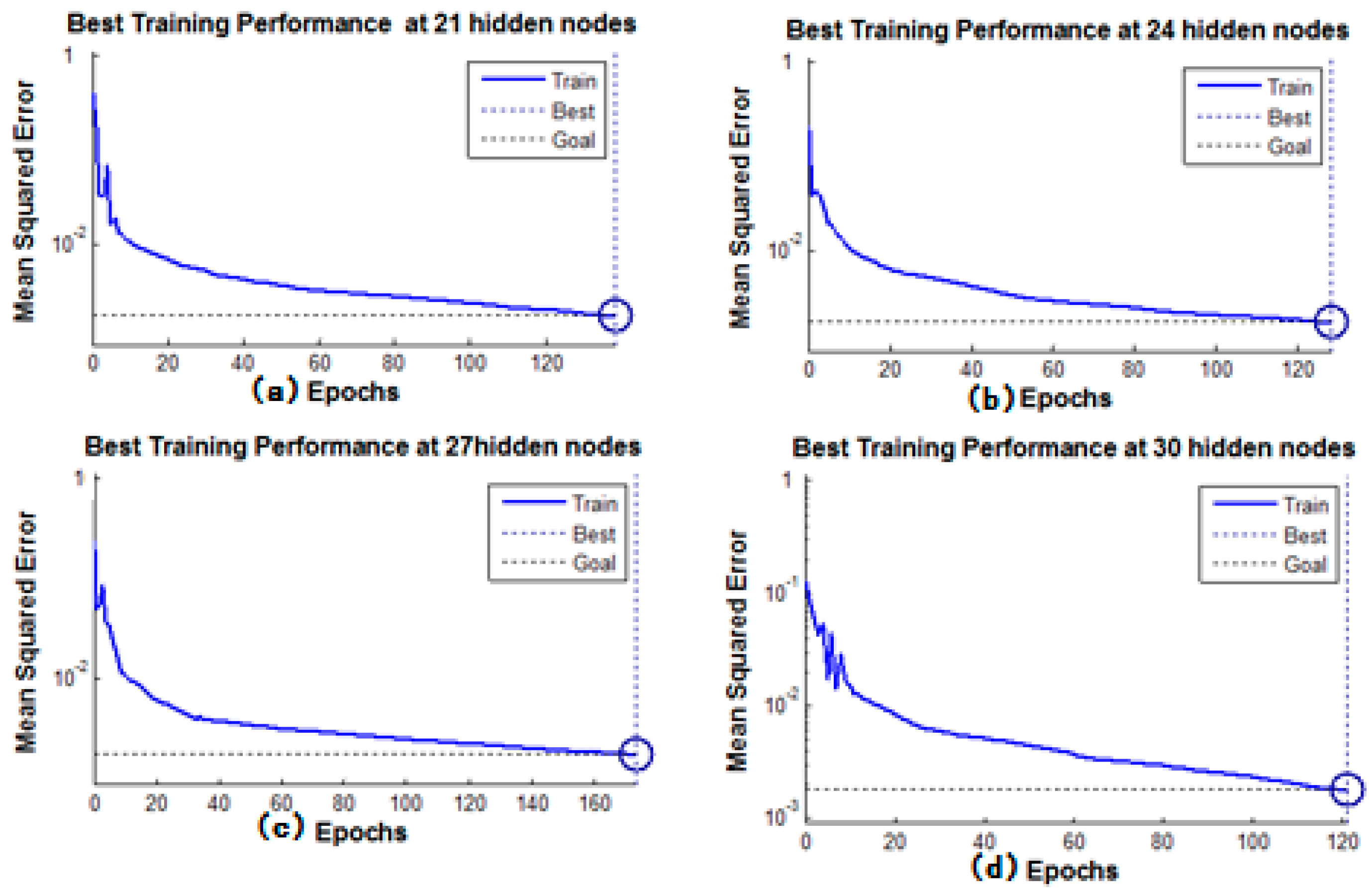
| Hidden Layer Number | Iteration Time (s) | Maximum Error for Training Set (%) | Maximum Error for Test Set (%) | Train Sample Number |
|---|---|---|---|---|
| 21 | 138 | 1.353 | 2.521 | 55 |
| 24 | 128 | 1.606 | 2.734 | 55 |
| 27 | 173 | 1.479 | 4.211 | 55 |
| 30 | 121 | 1.075 | 2.732 | 55 |
© 2016 by the authors; licensee MDPI, Basel, Switzerland. This article is an open access article distributed under the terms and conditions of the Creative Commons Attribution (CC-BY) license (http://creativecommons.org/licenses/by/4.0/).
Share and Cite
Zhang, J.; Tan, X. Quantitative Inspection of Remanence of Broken Wire Rope Based on Compressed Sensing. Sensors 2016, 16, 1366. https://doi.org/10.3390/s16091366
Zhang J, Tan X. Quantitative Inspection of Remanence of Broken Wire Rope Based on Compressed Sensing. Sensors. 2016; 16(9):1366. https://doi.org/10.3390/s16091366
Chicago/Turabian StyleZhang, Juwei, and Xiaojiang Tan. 2016. "Quantitative Inspection of Remanence of Broken Wire Rope Based on Compressed Sensing" Sensors 16, no. 9: 1366. https://doi.org/10.3390/s16091366