Review

A Comprehensive Review on Water Quality Parameters Estimation Using Remote Sensing Techniques

1
Department of Civil Engineering, Florida International University, Miami, FL 33174, USA
2
Department of Earth and Environment, Florida International University, Miami, FL 33199, USA
*
Author to whom correspondence should be addressed.
Sensors 2016, 16(8), 1298; https://doi.org/10.3390/s16081298
Submission received: 12 May 2016 / Revised: 1 August 2016 / Accepted: 8 August 2016 / Published: 16 August 2016
(This article belongs to the Special Issue Sensors and Sensing in Water Quality Assessment and Monitoring)

Abstract

:
Remotely sensed data can reinforce the abilities of water resources researchers and decision makers to monitor waterbodies more effectively. Remote sensing techniques have been widely used to measure the qualitative parameters of waterbodies (i.e., suspended sediments, colored dissolved organic matter (CDOM), chlorophyll-a, and pollutants). A large number of different sensors on board various satellites and other platforms, such as airplanes, are currently used to measure the amount of radiation at different wavelengths reflected from the water’s surface. In this review paper, various properties (spectral, spatial and temporal, etc.) of the more commonly employed spaceborne and airborne sensors are tabulated to be used as a sensor selection guide. Furthermore, this paper investigates the commonly used approaches and sensors employed in evaluating and quantifying the eleven water quality parameters. The parameters include: chlorophyll-a (chl-a), colored dissolved organic matters (CDOM), Secchi disk depth (SDD), turbidity, total suspended sediments (TSS), water temperature (WT), total phosphorus (TP), sea surface salinity (SSS), dissolved oxygen (DO), biochemical oxygen demand (BOD) and chemical oxygen demand (COD).

Graphical Abstract

1. Introduction

Over 40% of the world’s population lives in coastal regions and lake or river shores [1], and this proportion is increasing. The coastal area of rivers and other waterbodies are among the most sensitive environments. Any changes in these fragile ecosystems due to anthropogenic activities can endanger the habitats of fish and other aquatic organisms. Similarly, the need for sustainable urban water supplies requires that the quality of existing available water resources as well as their watersheds need to be under continuous monitoring. Besides, the level of treatment required for human consumption, agriculture, animal husbandry and industry necessitates an understanding of the quality of source waters. In this way, at the beginning of the twentieth century, the importance of water quality has to be considered more than ever, and the concentration of chemicals in sewage and industrial discharges in waterbodies needs to be taken under more precise control [2,3].
Water quality indicators including physical, chemical, and biological properties are traditionally determined by collecting samples from the field and then analysing the samples in the laboratory. Although this in-situ measurement offers high accuracy, it is a labour intensive and time consuming process, and hence it is not feasible to provide a simultaneous water quality database on a regional scale [4,5]. Moreover, conventional point sampling methods are not easily able to identify the spatial or temporal variations in water quality which is vital for comprehensive assessment and management of waterbodies. Therefore, these difficulties of successive and integrated sampling become a significant obstacle to the monitoring and management of water quality.
With advances in space science and the increasing use of computer applications and increased computing powers over recent decades, remote sensing techniques have become useful tools to achieve this goal. Remote sensing techniques make it possible to monitor and identify large scale regions and waterbodies that suffer from qualitative problems in a more effective and efficient manner. The collection of remotely sensed data occurs in digital form and therefore is easily readable in computer processing. Remote sensing techniques have been in use since the 1970’s and continue to be widely used in water quality assessment in the contemporary world [6,7,8,9,10,11,12,13,14,15,16,17,18,19,20,21].
Different sensors mounted on satellites and other platforms, such as aeroplanes, measure the amount of radiation at various wavelengths reflected from the water’s surface. These reflections can be used directly or indirectly to detect different water quality indicators, such as total suspended solids (TSS), chlorophyll-a concentration, turbidity, salinity, total phosphorus (TP), Secchi disk depth (SDD), Temperature, pH, Dissolved Organic Carbon (DOC),etc. The spectral characteristics of water and pollutants, which are functions of the hydrological, biological and chemical characteristics of water, etc. [19], are essential factors in the monitoring and assessment of water quality. The study thus introduces the widely employed spaceborne and airborne sensors in water quality investigations and discusses the utility of remotely sensed techniques in the qualitative assessment of waterbodies. Various properties (spectral, spatial and temporal, etc.) of spaceborne and airborne sensors are tabulated to be used as a sensor selection guide. Finally, based on the literature survey, the study presents a compilation of the various sensors useful in the study of some measurable water quality parameters, and investigates in more detail eleven water quality parameters based on the employed approaches to measuring their concentrations.

2. An Overview of Water Quality Assessment and Remote Sensing

In-situ data collections are only able to represent point estimations of the quality of water conditions in time and space, and obtaining spatial and temporal variations of quality indices in large waterbodies is almost impossible [18]. Briefly listed below are the most important limitations associated with conventional methods:
  • In-situ sampling and measurements of water quality parameters are labor intensive, time consuming, and costly.
  • Investigation of the spatial and temporal variations and water quality trends in large waterbodies is almost impossible.
  • Monitoring, forecasting, and management of entire waterbodies might be inaccessible, for example due to the topographic situation.
  • Accuracy and precision of collected in-situ data can be questionable due to both field-sampling error and laboratory error.
To overcome these limitations, the use of remote sensing in water quality assessment can be a useful tool. For more than four decades, remote sensing has illustrated strong capabilities to monitor and evaluate the quality of inland waters. Many researchers frequently use the visible and near infrared bands of the solar spectrum (mostly from blue to near infrared region) in their investigations to obtain robust correlations between water column reflection (in some cases emission) and physical and biogeochemical constituents, such as transparency, chlorophyll concentration (phytoplankton), and the organic matters and mineral suspended sediments in different waterbodies [9,10,18,22,23,24,25,26,27,28,29,30]. Although the capabilities of remote sensing to assess water quality are undeniable, this technique alone is not sufficiently precise and must be used in conjunction with traditional sampling methods and field surveying. In other words, to obtain a better insight, an integrated use of remote sensing, in-situ measurements and computer water quality modelling may lead to an increased knowledge of the water quality of water systems. Collaboration between different governmental, federal and private agencies and data sharing is also helpful to increase the data required for regional studies. Kallio [31] has mentioned four advantages of applying remote sensing in compliance with other water quality monitoring programs as below:
  • Gives a synoptic view of the entire waterbody for more effective monitoring of the spatial and temporal variation.
  • Makes it possible to have a synchronized view of the water quality in a group of lakes over a vast region.
  • Provides a comprehensive historical record of water quality in an area and represents trends over time.
  • Prioritizes sampling locations and field surveying times.
Optically active constituents of water that interact with light and change the energy spectrum of reflected solar radiation from waterbodies can be measured using remote sensing [18]. The components, already enumerated in the first section, constitute the majority of important water quality parameters in surface waters. Other parameters include acidity, chemicals, and pathogens, which do not change the spectral properties of reflected light and have no directly-detectable signals, but which may be interpretable and inferable from those detectable water quality parameters with which strong correlations can be found [18,31].

3. Spaceborne and Airborne Sensors for Water Quality Studies

Observing sensors are divided into two main categories based on the platforms on which they are situated. Airborne sensors are those that are mounted on a platform within the Earth’s atmosphere (i.e., a boat, a balloon, a helicopter, or an aircraft), and spaceborne sensors are carried by a spacecraft or satellite to locations outside of the Earth’s atmosphere. Understanding the properties of these sensors is necessary to choose an appropriate sensor for the objectives of the study. Therefore, various remote sensing satellites (Table 1) and airborne systems (Table 2) commonly used in water quality assessments, along with their spectral properties including spatial resolution, spectral bands, and revisit interval are presented. This tabulated information is helpful when designing water quality assessment studies, and can be used for the selection of appropriate sensors among many other available sensors in the market.
Other categories of sensors that have broad applications in oceanographic remote-sensing are microwave radiometers (MWR) and synthetic aperture radar (SAR). Passive microwave radiometers measure energy emitted at sub-millimeter-to-centimeter wavelengths (at frequencies of 1–1000 GHz) known as microwaves. By understanding the physical processes associated with energy emission at these wavelengths, oceanographers can calculate two important water quality parameters, sea surface temperature (SST) and sea surface salinity (SSS). They have also been used for measuring atmospheric and terrestrial radiation, meteorological studies, such as zenith-pointing surface instruments that view the Earth's atmosphere in a region above the stationary instrument. Table 3 shows the characteristics of the more commonly used microwave radiometers in oceanography and water quality studies.
Synthetic aperture radar is a form of radar that used to create two or three-dimensional images of objects [32,33,34], and can be mounted on either an aircraft or spacecraft. Although SARs are widely used for water pollution detection like oil pollution, ocean topography, wind speed at the sea surface, and regional ice monitoring, they are not very often applied in water quality studies and measuring water quality parameters. In cases where the data from these sensors are combined with other sensors in water quality studies, the results have demonstrated that SARs are only marginally helpful in improving the estimation of water quality parameters; for example in Zhang [35] study.

4. Water Quality Investigations through Remote Sensing Techniques

Water quality study is the process of determining the chemical, physical and biological characteristics of waterbodies and identifying the possible contamination sources that degrade the quality of water [20]. Degradation of the quality of water resources may result from waste discharges, pesticides, heavy metals, nutrients, microorganisms, and sediments. Different water quality standards have been developed to aid in checking the extent of water pollution, and consequently to maintain these quality standards. The most commonly measured qualitative parameters of water are detailed in Table 4.
The terminology and rationale for Case 1 and Case 2 water classifications were established by Morel and Prieur [16] and Gordon and Morel [83] in their seminal work on the bio-optical basis for ocean color variations. The definition for Case 1 and Case 2 waters was updated by Mobley et al. [84] as follows:
  • Case 1 waters are those waters whose optical properties are determined primarily by phytoplankton and related colored dissolved organic matter (CDOM) and detritus degradation products.
  • Case 2 waters are everything else, namely waters whose optical properties are significantly influenced by other constituents such as mineral particles, CDOM, or microbubbles, whose concentrations do not covary with the phytoplankton concentration.
Remote sensing techniques make it possible to have spatial and temporal view of surface water quality parameters and more effectively and efficiently monitor the waterbodies, and quantify water quality issues. Most of the studies have focused on optically active variables, such as chlorophyll-a (chl-a), total suspended solids (TSS), and turbidity. There are several other important water quality variables such as pH, total nitrogen (TN), ammonia nitrogen (NH3-N), nitrate nitrogen (NO3-N), and dissolved phosphorus (DP), which existing literature omit. The main reason is due to their weak optical characteristics and low signal noise ratio. However, these parameters are an important part of water quality indices and are a challenging aspect of research in the field of water quality assessment using remote sensing, which should stimulate and motivate scientists in further efforts. In continuing, the study precisely surveys the more commonly employed approaches in estimating the concentration of the eleven water quality parameters. These water quality indicators include chlorophyll-a (chl-a), colored dissolved organic matters (CDOM), Secchi disk depth (SDD), turbidity, total suspended sediments (TSS), water temperature (WT), total phosphorus (TP), sea surface salinity (SSS), dissolved oxygen (DO), biochemical oxygen demand (BOD) and chemical oxygen demand (COD).

4.1. Chlorophyll-a

Algal blooms, which are often driven by eutrophication phenomena in freshwater, are directly related to chl-a concentration since it is essential for photosynthesis [36]. Chl-a is used in oxygenic photosynthesis and is found in plants, algae and cyanobacteria. Chl-a is the major indicator of trophic state because it acts as a link between nutrient concentration, particularly phosphorus, and algal production. Chl-
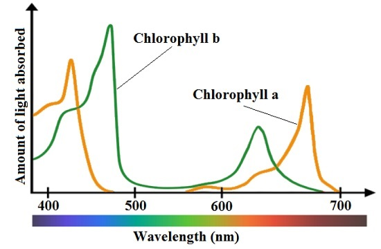
a while mainly reflecting green, absorbs most energy from wavelengths of violet-blue and orange-red light, whose reflectance causes chlorophyll to appear green. Obviously, the addition of chl-b besides chl-a extends the spectrum absorption. Low light conditions tends to favor the production, a rather greater ratio, of chl-b to chl-a molecules, thus increasing photosynthetic yield [85]. Figure 1 shows the absorption spectrum of both chl-a and chl-b pigments. Many researchers have demonstrated that increasing chl-a concentration causes a decrease in the spectral response at short wavelengths, particularly in the blue band [86,87,88,89,90,91]. A large number of studies have focused on chl-a concentration measurement using remote sensing, some of which are cited in this review paper.
Narrow bands of imagery are required for the measurement of chl-a concentration and its spatial and temporal variations within a waterbody [92]. A review of the literature on the application of empirical approaches using multispectral sensors shows ambiguous results. While estimating chlorophyll using remote sensing techniques is possible and a lot of authors claim to achieve satisfying results using broadband sensors, several studies exist showed that the broad wavelength spectral data available on current satellites (i.e., Landsat, SPOT) do not permit discrimination of chlorophyll in waters with high suspended sediments [86]. This is especially due to the dominance of the spectral signal from the suspended sediments, more so in highly turbid and eutrophic waters [93,94].
Since the late 1970’s, many researchers developed bio-optical algorithms that initially were designed for oceans to determine water quality parameters. In these waterbodies, phytoplankton and its breakdown products are the sole determinants of optical properties of the water. In Case 1 waters, by employing an empirical model and interpreting the received radiance at different wavelengths, the concentrations of chl-a can be adequately estimated with satellite images [83]. In Case 1 waters, spectral bands in the blue to green region are appropriate to identify chl-a concentrations with acceptable precisions. However, in Case 2 waters due to the complexity of the constituents in water, the detection of chl-a is a sophisticated task and requires advanced approaches and techniques. In Case 2 waters (inland and coastal waters), the optical properties are determined, additionally to phytoplankton, by a composite of dissolved organic matter from a terrestrial origin, dead particulate organic matter and inorganic particulate matter. Therefore, determination of chl-a concentration is much more complex and less accurate as these constituents are not statistically correlated. Additionally, the simple fact that Gelbstoff absorption often masks the blue-green region in Case 2 waters implies chl-a algorithms developed for Case 1 waters are not applicable to Case 2 waters [95].
Various visual spectral bands and their ratios are widely used to quantify chl-a. Spectral band ratios can reduce irradiance, atmospheric and air-water surface influences in the remotely sensed signal [86,96]. The prominent scattering-absorption features of chl-a include strong absorption between 450–475 nm (blue) and at 670 nm (red), and reflectance reaches to peak at 550 nm (green) and near 700 nm (NIR). The reflectance peak near 700 nm and its ratio to the reflectance at 670 nm have been used to develop a variety of algorithms to retrieve chl-a in turbid waters [23]. Gitelson [97] studied the behavior of the reflectance peak near 700 nm and concluded that the 700 nm reflectance peak was important for the remote sensing of inland and coastal waters, especially for measuring chlorophyll concentration. Han [98] pointed out that the spectral regions at 630–645 nm, 660–670 nm, 680–687 nm and 700–735 nm were found to be potential regions where the first derivatives can be used to estimate chlorophyll concentration. Dekker et al. [99] mentioned that the scattering and absorption characteristics of chl-a can be studied when more than one band is used. Hoogenboom et al. [100] noted that a ratio using an Advanced Visible–Infrared Imaging Spectrometer (AVIRIS) band located near 713 nm along with the band at 667 nm was the most sensitive for chlorophyll retrieval in inland waters. A similar ratio (R674/R705) has been demonstrated to be optimal for inland lakes and rivers [101]. Table 5 shows some of the more commonly used techniques for the measurement of chl-a concentration.
Other significant literature that applied other approaches to the measurement of chl-a are considered hereafter. Alparslan, Coskun and Alganci [61] measured the concentration of chl-a using all bands of Landsat-5 TM. Ekercin [128] used Band 1 (445–530 nm), Band 2 (520–610 nm), Band 3 (640–720 nm), and Band 4 (770–880 nm) of IKONOS data to estimate chl-a concentration in Istanbul, Turkey. Also, Nas, Karabork, Ekercin and Berktay [67] used the visible near-infrared (VNIR) and the shortwave infrared (SWIR) (first four bands 0.52–1.70 µm) of Terra/ASTER and developed a multiple regression between chl-a concentration and spectral reflectance in the Beysehir Lake, Turkey. Shafique, Fulk, Autrey and Flotemersch [29], using Compact Airborne Spectrographic Imager (CASI) studied the chl-a concentration in the Great Miami River and 80 miles of the Ohio River. They concluded that linear models using the ratio of wavelengths 705/675 nm could describe chl-a concentration. Bhatti, Rundquist, Schalles and Ramirez [40], using Airborne Imaging Spectroradiometer for Applications (AISA) sensor in the Apalachicola Bay in Florida, USA, found that two bands reflectance ratio R70 Other significant literature that applied other approaches to the measurement of chl-a are considered in following. Alparslan, Coskun and Alganci [61] measured the concentration of chl-a using all bands of Landsat-5 TM. Ekercin [128] used Band 1 (445–530 nm), Band 2 (520–610 nm), Band 3 (640–720 nm), and Band 4 (770–880 nm) of IKONOS data to estimate chl-a concentration in Istanbul, Turkey. Also, Nas, Karabork, Ekercin and Berktay [67] used the visible near-infrared (VNIR) and the shortwave infrared (SWIR) (first four bands 0.52–1.70 µm) of Terra/ASTER and developed a multiple regression between chl-a concentration and spectral reflectance in the Beysehir Lake, Turkey. Shafique, Fulk, Autrey and Flotemersch [29], using Compact Airborne Spectrographic Imager (CASI) studied the chl-a concentration in the Great Miami River and 80 miles of the Ohio River. They concluded that linear models using the ratio of wavelengths 705/675 nm can describe chl-a concentration. Bhatti, Rundquist, Schalles and Ramirez [40], using Airborne Imaging Spectroradiometer for Applications (AISA) sensor in the Apalachicola Bay in Florida, USA, found a significant correlation between the two bands reflectance ratio R700/R670 and chl-a concentration. Also, the three band model R750 * (R6701 − R7001) was found to be a predictor of chl-a concentration in Case 2 waters. In addition, the logarithmic ratio of ALOS/AVNIR-2 (Band 3/Band 1) was related with chl-a concentration in his study area. Lim and Choi [36] using Landsat-8/OLI showed that chl-a presented a good correlation with both OLI bands and band ratio, with calculated R values for Bands 2, 3, 4 and band ratio (Band 5/Band 3) as −0.66, −0.70, −0.64, and −0.64, respectively, at a significance level of p < 0.01. ZHANG and HAN [129] found that OLI bands 1 to 4 and their combinations had good correlation with chl-a concentration. Kim et al. [130] using Landsat-8/OLI employed Band 2, Band 5, and a ratio of Band 2/Band 4 to measure chl-a concentration. Mannheim et al. [131] found that the reflectance curve and the baseline from 672 to 742 nm (CHRIS spectral Bands 8–12) shows the best correlation results and the maximal sensitivity to variations of chl-a concentration. Choe et al. [132] used Moderate Resolution Imaging Spectroradiometer (MODIS), Sea-viewing Wide Field-of-view Sensor (SeaWiFS), Medium Resolution Imaging Spectrometer (MERIS), and RapidEye for the estimation of chl-a concentration in turbid waters using Two-band and Three-band models based on band ratio such as Red and NIR band.
Furthermore, Qi et al. [133] developed an approach based on Empirical Orthogonal Function (EOF) analysis to estimate chl-a concentration in surface waters of Taihu Lake, the third largest freshwater lake in China. The EOF approach analyzed the spectral variance of normalized Rayleigh-corrected reflectance (Rrc) data at 469, 555, 645, and 859 nm, and subsequently related that variance to chl-a using 28 concurrent MODIS and field measurements. Feng et al. [134] developed a new empirical chl-a algorithm for the largest freshwater lake of China (Poyang Lake) using a normalized green-red difference index (NGRDI) and atmospherically-corrected Medium Resolution Imaging Spectrometer (MERIS) data.
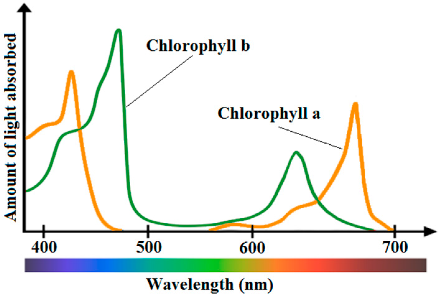
Reviewing the literature showed that most algorithms to determine the chl-a concentration need a wavelength near 675 nm and another near 700 nm. For example, the positioning of the spectral bands of Landsat/ETM+ is illustrated in Figure 2. This figure reveals that the bands are not very broad and also not suitably positioned for the detection of chl-a. Other multispectral sensors such as ASTER, IRS-LISS III and SPOT-HRV have similar spectral positioning in the Red/NIR region and therefore one can conclude that neither of these sensors is very appropriate for the detection of chl-a.
As mentioned, several satellite and airborne imageries can be used for chl-a estimation. Nonetheless, it revealed that the Landsat TM seems to be more appropriate and widely used for chl-a assessment. Temporal coverage and spatial resolution of TM and its easy accessibility can be the main reasons for the selection of this sensor.

4.2. Colored Dissolved Organic Matters (CDOM)

Colored Dissolved Organic Matters, also called gelbstoff and gilvin, consists of naturally occurring, water-soluble, biogenic, heterogeneous organic substances that are yellow to brown in color [135], which exist in both fresh and saline waters. These compounds are brown and can color the water yellowish brown in high concentrations. Therefore, they are referred to as yellow matter or colored dissolved organic matter (CDOM), and usually with chl-a and TSS dominate the water color.
CDOM absorbance spectrum can be several times and overlaps the chlorophyll absorption and can account for over 50% of the total absorption at 443 nm, which is the wavelength that chlorophyll concentrations are usually measured [136]. The increase in the CDOM concentration mainly affects the reflectance values in the blue and green region of the spectrum (especially below ~500 nm) and its absorbance increases exponentially with decreasing wavelength. This effect can complicate the use of chl-a retrieval algorithms and phytoplankton production models that are based on remotely sensed ocean color [137]. Nonetheless, it is reported by Strömbeck and Pierson [138] that at high CDOM concentrations, absorbance of red light spectrum can be significant.
Remote sensing of CDOM is important in studying aquatic ecology and carbon dynamics [18,139]. Existence of CDOM in rivers, lakes, and oceans affects the water color as seen by many satellite remote sensing instruments, such as MODIS and SeaWiFS [140]. CDOM also affects the underwater light field and water’s inherent optical properties (IOP). This characteristic determines the water reflectance received by remote sensors. Therefore, inversion of remote sensing data provides an efficient method to estimate CDOM concentration within a large spatial and temporal scale [141,142]. In ocean color studies, CDOM absorption properties, for example, its absorption coefficients at 440 nm, are usually used as a representative of CDOM concentration [143]. In the algorithms derived from sensors like CZCS, chl-a concentrations were empirically inverted, and accordingly, CDOM can be measured with the assumption that it co-varies with chlorophyll [16,83,144]. Hyperspectral measurements with newly developed remote sensing reflectance models [145] have also been used to estimate CDOM as one of ocean color components, such as EO-1 Hyperion with MIM (Matrix Inversion Method) [8]. Kutser et al. [146] also used band ratio of EO-1/ALI Band 2 and Band 3 to estimate CDOM content in lakes of Southern Finland.
Recent approaches of CDOM estimation combine hyperspectral remote sensing data with semi-analytical models, new factors like the bottom effects, and computational techniques to enhance the accuracy of CDOM inversion [49]. Traditionally, in most water quality monitoring programs, CDOM absorption is referred to as color and PCU color (Platinum-Cobalt Units) and is used to characterize it. In recent studies, CDOM absorption is directly reported as light absorption coefficients at given wavelengths, and these absorption coefficients and PCU colors are closely correlated [136]. Semi-analytical models have been developed and applied to SeaWiFS (Sea-viewing Wide Field-of-view Sensor) and MODIS (Moderate Resolution Imaging Spectroradiometer), in which CDOM’s absorption coefficients are directly and independently inverted from remote sensing reflectance (Rrs) [49]. The semi-analytical models are based on the radiative transfer equations as well as the simplification of radiance and underwater light field [142]. Remote sensing of CDOM in riverine waters and coastal waters is a challenge and subject to large errors compared to oceanic waters because spectral signals of CDOM usually interfere with chlorophyll and suspended sediments [54,147]. In these complex environments, hyperspectral remote sensing present an advantage due to their spectral responses to water inherent optical properties (IOP) and their broad spectrum of narrow bands.
Several studies have confirmed that high spectral resolution (10 nm or better) can improve the estimation of water inherent optical properties (IOP) in coastal water [8,148,149]. However, as mentioned, due to the spectral signal interference from chlorophyll, suspended sediments as well as spatial and temporal heterogeneity of riverine and coastal waters, the applicable bands for CDOM measurement are not always at the same wavelengths. Therefore, identification of significant wavelengths out of hundreds of narrow bands of hyperspectral reflectance is a challenging task [55]. As a solution, first, the dimensionality of hyperspectral data should be reduced through techniques such as band selection, derivative analysis, spectral indices, or hyperspectral transformation [122,150,151,152]. It is also necessary to calibrate and validate the remotely sensed CDOM concentrations using a shipboard data acquisition approach concurrently with high spatial resolution underwater CDOM observation. Additionally, CDOM is reported to be commonly used as an important indicator for dissolved organic carbon (DOC) dynamics in freshwater and coastal marine ecosystems [153] and many observations have provided evidence that CDOM is correlated to DOC [54,154,155,156,157,158]. Reviewing the literature revealed that most of the studies are based on four sections: underwater CDOM measurements, in situ hyperspectral measurements, water-surface reflected radiance by means of remote sensor on a satellite or an airborne platform, and functional data analysis [49,153]. The literature showed that CDOM could be quantified using visual spectral bands and their ratios, which is as summarized in Table 6.
Furthermore, Taheri Shahraiyni et al. [174] by using reflectance values at 490, 510, 560, 620, and 885 nm of MERIS data and applying a fuzzy modeling technique, Active Learning Method (ALM), mapped the spatial distribution of CDOM over the southern parts of the Caspian Sea, Iran. A proxy algorithm was reported for remote sensing of CDOM by an absorption coefficient of ocean water, which is a multi-band quasi-analytical algorithm (QAA) developed by Lee, Carder and Arnone [141]. Further, alternative algorithms such as computer-based discrete modelling methods are developed for remote sensing of CDOM. However, Kishino et al. [175] expressed that results can be questionable when a neural network model is implemented to measure the CDOM concentration using ASTER data. Johannessen et al. [176] using SeaWiFS images found out a relationship between ultraviolet (UV) attenuation coefficient (Kd) at 323 nm, 338 nm, and 380 nm and the Rrs(412)/Rrs(555) band ratio.
Researchers use many sensors to assess CDOM, but SeaWIFS and MODIS, because of their coarse spatial resolution, were widely applied in deep waters. Due to the need for high accuracy for large-scale applications, SeaWiFS data are of little use in shallow waters and hyperspectral imagery like EO-1/Hyperion, EO-1/ALI, and ALOS/AVNIR-2 were preferable for these areas. In addition, a majority of researchers have used a high-resolution spectroradiometer in their in situ hyperspectral measurements to validate their quantified results. These in situ measurements include reflectance values collected at a single certain location and often used as an indicative of individual targets. These data are useful in identifying concentrations of components within the water column and can be collected above and below the water surface [22]. They are also useful for calibration and validation of remotely sensed estimations of water quality parameters.

4.3. Secchi Disk Depth

Secchi depth is an optical property of water strongly related to water constituents present in the waterbodies. The Secchi depth exhibits an inverse correlation with the amount of total suspended solids (TSS) present in the waterbodies. It can be used to study the relative nutrient and solids loading situations [177]. The most commonly attempted method for the measurement of water transparency is based on light attenuation principles [
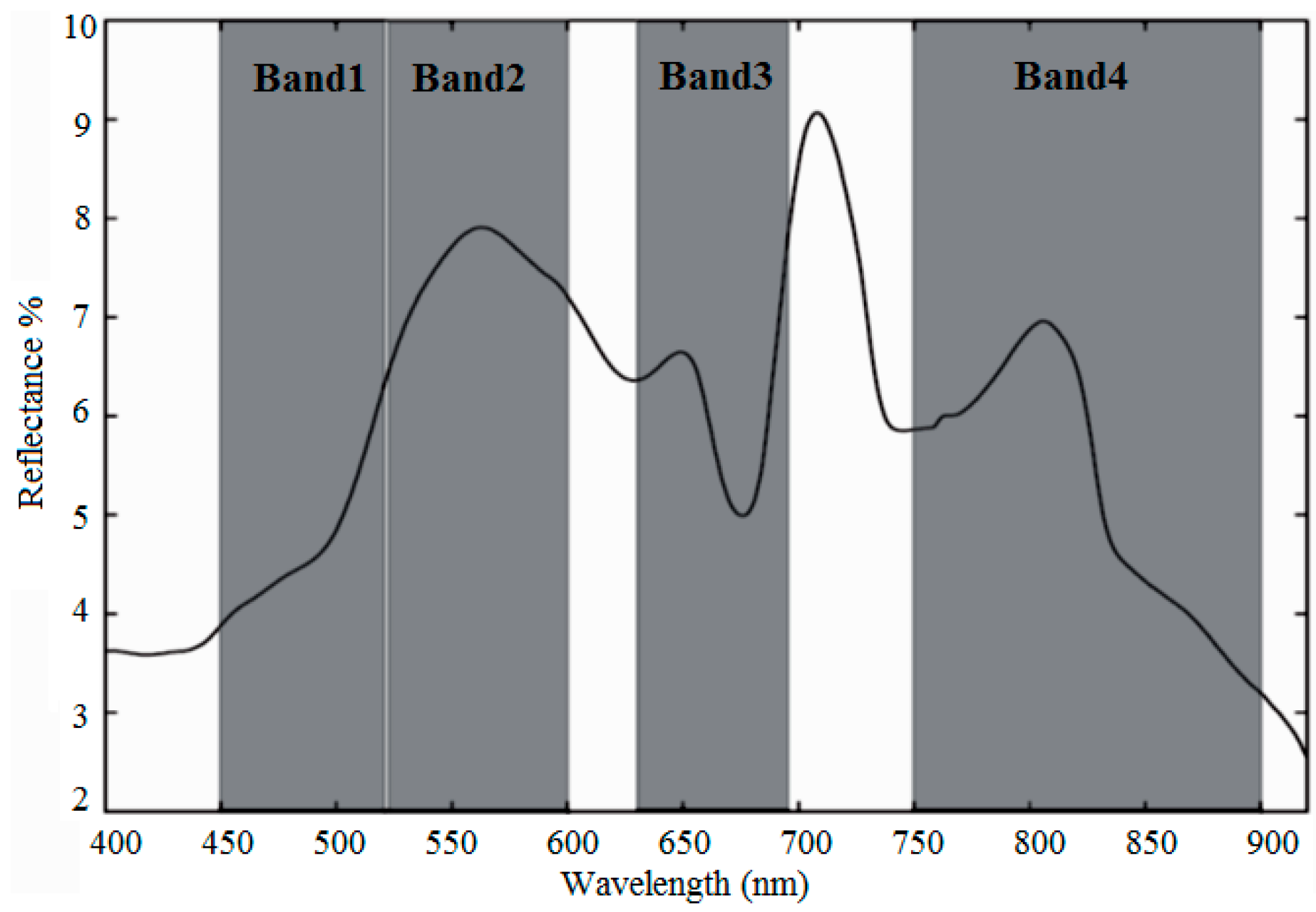
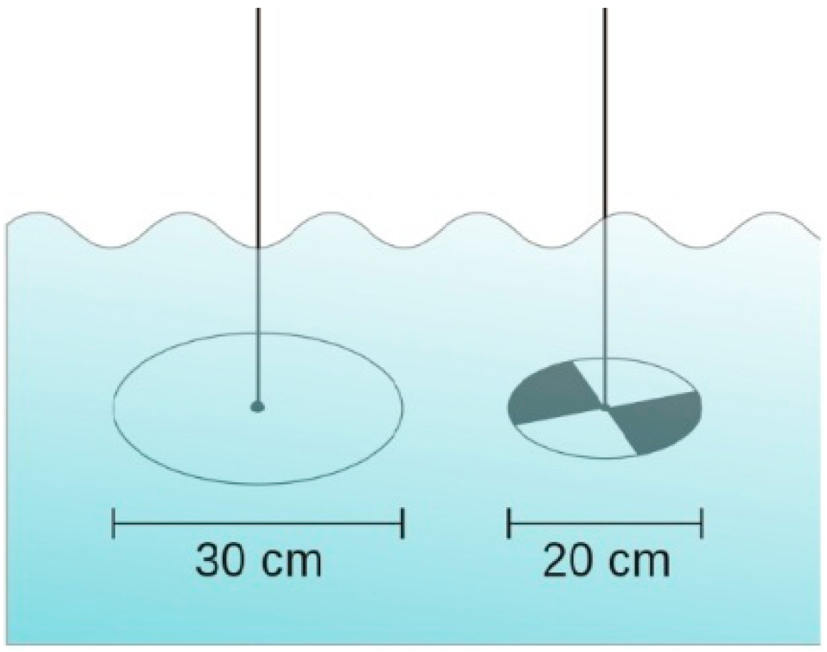
142]. The best-known operational estimation of water transparency is the Secchi disk, created by Pietro Angelo Secchi SJ in 1865, and is a circular disk used for clarity measurements in oceans and lakes. The disc mounts on a line and lowers slowly down in the water until the pattern on the disk is no longer visible. This measure is known as the Secchi disk depth (SDD) and is also related to water turbidity. Figure 3 shows two different kinds of Secchi disks.
SDD is a reasonable indicator of trophic conditions (algal abundance) except in highly colored lakes with low chl-a and non-algal turbidity (clay, calcium carbonate) [42]. The Secchi depth is inversely correlated with the amount of TSS present in the waterbodies. Therefore, remote sensing can be an ideal tool for monitoring water transparency and estimating the SDD. Recently, Lee et al. [178] introduced a model to estimate the SDD, which unlike the classical model that relies strongly on the beam attenuation coefficient, the new model relies only on the diffuse attenuation coefficient at a wavelength corresponding to the maximum transparency for such interpretations. Many researchers have applied remote sensing for this purpose and have shown in their studies that remote sensing data is well correlated with SDD values [179,180,181,182].
SDD has a significant correlation with atmospherically corrected satellite radiance [184,185,186]. In atmospherically corrected MSS Green band, SDD is related to reflectance just below the surface, incorporating the ratio of backscattering to total scattering coefficients for suspended particles [187]. The relationship is quite accurate for SDD < 16 m [188]. Significant algorithms have been developed for SDD using various remote sensing data, like TM [27,39,102,189,190], MSS [24,25,191,192,193], IKONOS [28,60,128] and even video data [194]. Landsat-TM is one of the most frequently used sensors to estimate SDD. Braga et al. [195] found that SDD was closely correlated with TM data, especially during high tide. Furthermore, highly suitable models were developed for SDD that ranged from 4 to 15 m from TM1 and TM3 satellite radiance [186]. However, there was an exception research conducted by Lopez-Garcia and Caselles [124]. They used TM data and reported that SDD did not show significant correlation with any TM bands. SDD can also be quantified from reflected radiance received by the IRS satellite [184].
There are many established relationships in the literature between Secchi depth and total phosphorus, chl-a, TSS, and CDOM. The existing literature showed that SDD can be quantified using visual spectral bands and various band ratios. Bhatti, Rundquist, Schalles and Ramirez [40] used ALOS-AVNIR-2 data and found that the Secchi depth was well correlated with reflectance ratio of R750/R560 (NIR/Green). Thiemann and Kaufmann [101] used HyMap and CASI data for Secchi disk transparency and chlorophyll-a determination in the Mecklenburg Lake District, Germany. They used the area between a base line and the spectrum from 400 to 750 nm and found a good correlation with the in situ measured Secchi disk transparency (SDT). Ekercin [128] using Band 1 (445–530 nm), Band 2 (520–610 nm), and Band 3 (640–720 nm) of IKONOS data and developed an algorithm for SDD measurements. Mancino, Nolè, Urbano, Amato and Ferrara [26] developed an equation using TM1 and the TM3/TM2, TM1/TM2, TM2/TM1 ratios, and Powell et al. [196] suggested a regression equation related to in-situ Secchi disk transparency measurements by using the Blue, Green, and Red bands of TM. In addition, based on Kloiber et al. (2002) study and TM and MSS imagery analysis, some recommendations were made for a Landsat-based procedure of water clarity assessment. Literature also showed that Secchi disk depth can be quantified using visual spectral bands and various band ratios, which are summarized in Table 7.
Although several satellite remote sensing systems have been used to measure the SDD, the relatively low cost, temporal coverage, spatial resolution, and data availability of the Landsat system make it particularly most useful data for the assessment of this water quality parameter. Several studies have demonstrated a strong relationship between Landsat Multispectral Scanner (MSS) or Thematic Mapper (TM) data and ground observations of Secchi depth, which are cited earlier.
SDD and chl-a concentrations have been successfully predicted from satellite image data by developing the relationship between in-situ measurements of SDD and chl-a, and the spectral response of the blue, green, red, and near-infrared bands. This approach has been successfully implemented in Minnesota [202], Wisconsin [203], and Michigan [204] to estimate water clarity for inland lakes, where in-situ data is limited.

4.4. Turbidity and Total Suspended Sediments

Water turbidity is an optical property of water, which scatters and absorbs the light rather than transmit it in straight lines. Suspended sediments are responsible for most of the scattering, whereas the absorption is controlled by chl-a and colored dissolved or particulate matter [205]. As water turbidity is mainly the result of the presence of suspended matter, turbidity measurement has often been used to calculate fluvial suspended sediment concentrations [206] and is commonly regarded as the opposite of clarity. The level of turbidity or murkiness is entirely dependent on the amount of suspended particles in a sample of water. The more suspended particles, the more difficult for light to travel through the water and therefore, the higher the water’s turbidity. The complex nature of suspended substances in water changes the reflectance of the waterbody and therefore causes variation in color. To this end, interpretation of remotely sensed data just based on the color of water is not adequate and accurate. Turbidity and total suspended matters are considered as important variables in many studies due to their linkage with incoming sunlight that in turn affects photosynthesis for growth of algae and plankton. These parameters are also directly associated with Secchi disk depth.
Remote sensing techniques are widely used to estimate and map the turbidity and concentrations of suspended particles, and to provide their spatial and temporal variations. Theory shows that use of a single band provides a robust and TSM-sensitive algorithm provided the band is chosen appropriately [207]. Curran et al. [208] and Novo et al. [209] showed that single band algorithms may be adopted where TSM increases with increasing reflectance. However, the complex substances in water change the reflectance of the water body and therefore cause variation in colors, and thus, different spectral bands can be used for TSS retrievals [207,210,211]. For example, high levels of total suspended solids or the presence of dark-colored humus acids from the decay of vegetation, common in the water of peat bogs, would result in high TSS and turbidity readings (Mark and Stapp, 2003). Therefore, the advantage of using signal band or band ratios can be employed to obtain more accurate results in different concentrations in waterbodies. In the Near-IR and Mid-IR regions, water increasingly absorbs the light and makes it look darker, which varies based on water depth and wavelength. An increase of dissolved inorganic materials in waterbodies causes the peak of visible reflectance to shift from the green region (clearer water) toward the red region of the spectrum. Several studies have also found that the first four bands of Landsat are well correlated with total suspended matters [42,198,212,213]. However, Ritchie et al. [214] by in situ studies showed that the most useful range of spectrum for the determination of suspended particles in surface waters was between 700 and 800 nm. The literature showed that turbidity and/or Suspended Sediments can be measured using visual spectral bands and various band ratios, which are as summarized in Table 8.
Furthermore, Ekercin [128] used Band 1 (445–530 nm), Band 2 (520–610 nm), Band 3 (640–720 nm), and Band 4 (770–880 nm) of IKONOS data and estimated the concentration of TSS in Istanbul, Turkey. Alparslan, Coskun and Alganci [61] obtained the amount of turbidity from Band 1, Band 2, Band 3, Band 4, Band 5 and Band 7 of Landsat-5 TM Satellite Image. He, Chen, Liu and Chen [73] used a combination of Landsat TM Bands 2, 3, 6 and 7 to correlate with the in situ turbidity measurements. Also, Sudheer, Chaubey and Garg [58] suggested that a combination of TM1, TM2, TM3 and TM4 was significant to retrieve suspended sediments information from remote sensing data. Bhatti, Rundquist, Schalles and Ramirez [40] by using NIR/Green band ratio of ALOS-AVNIR-2 developed a relationship to calculate total suspended matters. Lim and Choi [36] found that suspended solids was correlated with Bands 2–5 of Landsat-8/OLI, and constructed 3 multiple regression models through single bands of OLI.
Reviewing the literature demonstrated that the Landsat/TM was used much more than other sensors. For rivers and other case studies that need more spectral and spatial resolution, ALOS/AVNIR-2, IKONOS on spaceborne sensors, and CASI and AISA hyperspectral imagery on airborne sensors were used to determine turbidity and suspended matters. The methodology to interpret images and to evaluate the turbidity was also improved from simple linear regression to non-linear multiple regression, principle components analysis (PCA) and neural networks.

4.5. Total Phosphorus

Total phosphorus (TP) studies consist of the measurement of all inorganic, organic and dissolved forms of phosphorus. Phosphates are plant nutrients whose increased quantity helps plants and algae to grow quickly. Total phosphorus can be directly related to chl-a concentration and indirectly related to transparency or water clarity, which is estimated by Secchi depth [218]. Rivers that flow through various land use activities can include different substances and chemicals like total suspended sediments, nutrients, residential fallout, and others. When a river or a creek passes through an agricultural area, for instance, the phosphorus load may show a higher concentration compared to other parameters present in the surface water. Fertilizer-rich agricultural runoffs and effluents from wastewater treatment plants are the main sources of high phosphorus and nitrogen concentrations in surface waters that threaten many worldwide ecosystems [219]. Total suspended matters usually act as a carrier for TP and also closely related to Secchi disk transparency with an exponential equation [220].
The measurement of total phosphorus concentrations in waterbodies is challenging due to the spatial heterogeneity and the labor-intensive collection and testing of required field samples. Remote sensing as a robust tool has already been used successfully to monitor water quality parameters in various scales and areas, although it presents a challenge in estimating phosphorus concentration. Remote estimation of total phosphorus (TP) has been investigated based on its high correlation with optically active constituents [69,220,221,222,223,224]. Total phosphorus is not directly measurable by optical instruments, but has a general correlation with other water quality parameters. As mentioned above, TP is closely related to some other parameters like phytoplankton [220,223], turbidity and total suspended matters (TSM), and Secchi disk transparency (SDT) [224], which is the basis for remote monitoring of TP dynamics [225]. Multispectral Landsat TM data have been widely used to monitor and map the TP spatial and temporal pattern in different regions [69,221,222]. Hyperspectral airborne or spaceborne remote sensing due to its finer diagnostic spectral band(s) provides more potential to detect TP in rivers and small lakes.
Many studies have shown that increasing the TP concentration in waterbodies results in a general tendency of increase in chl-a concentration [226,227,228,229]. Schindler [230] showed that 74% of the variability in chl-a concentration among lakes has a direct correlation with the variation of phosphorus concentration. His result suggests that chl-a concentration may play a role as a proxy of phosphorus concentration in waterbodies. In another study conducted by Heiskary and Wilson [231], the Secchi disk depth was decreased with increasing TP concentration that proved that a proportion of phosphorus can be attached to suspended particles resulted from soil erosion and transferred through river’s downslope. These studies suggested that both chl-a concentration and SDD are closely correlated with TP concentration [220] and therefore can be used as the potential theoretical parameters for the indirect prediction of TP concentration.
Table 9 shows a number of investigations to measure total phosphorus by applying blue band (0.45–0.51 μm) and green band (0.50–0.60 μm), and integration of red (0.60–0.70 μm) and green (0.50–0.60 μm) ratio from different sensors. Empirical estimations and various statistical regression models were used to correlate phosphorus concentration with other water quality indicators, such as Secchi depth (SD) and chl-a concentration. In addition, Bistani [232] using EO-1/Hyperion obtained a reflectance determination coefficient of 0.49 from the 467 to 529 nm bands ratio values, from which he derived a polynomial algorithm used to produce a total phosphorus distribution map. Song et al. [233] studied the correlation between TP and TM1, TM2, TM3, and TM4 from the Landsat 5, and found that each band had a correlation with TP of 0.62, 0.59, 0.55, and 0.51, respectively. Later in another study, Song, Li, Li, Tedesco, Hall and Li [68] by using the airborne imaging data (AISA), and applying red band (around 690 μm) and NIR spectral region (around 710 μm) estimated the total phosphorus (TP) in three central Indiana water supply reservoirs. Wu, Wu, Qi, Zhang, Huang, Lou and Chen [69] used a combination of TM1, TM3/TM2, and TM1/TM3 data to correlate chl-a concentration and SD measurements with TP concentration. Also, Alparslan, Coskun and Alganci [61] using Band 1, Band 2, Band 3, Band 4, Band 5 and Band 7 of Landsat-5 TM Satellite Image obtained the amount of total phosphorus concentration. Lim and Choi [36] used Bands 2, 3, 4, and 5 of Landsat-8/OLI, and constructed 3 multiple regression models by selecting both single bands and band ratios, and obtained significant correlation coefficients.
Results from studied articles indicate that there is a potential to estimate total phosphorus concentration at different scales using airborne and satellite images. The Landsat/TM was used much more than other sensors for TP assessment in the reviewed literature. As phosphorus does not directly present optically diagnostic signals in water leaving radiance for the water quality remote sensing spectral domain (400–900 nm), thus empirical modeling is considered the most applicable approach for the remote estimation of TP in water column [68,69,235]. The literature review also showed that TP has a similar spatial pattern to chl-a and SD concentration due to a high correlation of TP with these parameters. Total phosphorus also was highly related to sediment loadings. However, there is a time lag for phytoplankton to consume TP in reservoirs, which make the relationship between TP and chl-a or SD and total suspended sediments more complicated [68].
Light reflection from the bottom in shallow waters cannot be very reliable, because it may be a result of the above-water remotely sensed reflectance spectra. Therefore, the TP concentration estimated in shallow water may be questionable and needs to be validated using in situ data. Spatial and temporal distribution algorithms for TP concentration produced from satellite-based observations should also be verified by in situ measurements. These empirical methods provide site-specific predictions of total phosphorus with reasonable accuracy [236].

4.6. Water Temperature

Water temperature is an important parameter for the physical and biochemical processes occurring within water as well as in air-water interactions because temperature regulates physical, chemical, and biological processes in water. Water temperature also influences the solubility, and thus availability of various chemical constituents in water. Most importantly, this parameter affects dissolved oxygen concentrations in water; as oxygen solubility decreases with increasing water temperature. It is also very important to analyze the temporal variations due to seasonal changes. On the other hand, distribution, transportation, and interaction of some contaminants, such as nutrients have a significant relation with water column temperature.
Thermal infrared bands are able to measure the amount of infrared radiant heat emitted from land surfaces and the radiant temperature of waterbodies that have environmental and economic import. As thermal infrared is emitted from the surface, temperature estimations derived by remote sensing must be evaluated with great care when there are reasons to assume that the water is stratified [237], which occurs shortly after precipitation or solar warming and in areas influenced by freshwater runoff. In such cases, no relation can be expected between sea surface temperatures and the temperatures found in the water under the surface. Thermal stratification in freely flowing rivers is inherently unstable due to variations in channel shape, and in-stream objects, which cause a turbulent flow regime and can usually be detected in the imagery [238].
Remote sensing of water temperature in rivers is more complex than in other waterbodies because of their much smaller dimensions and difficulties of determination at the resolution (pixel size) of the thermal-infrared (TIR) data [45]. Stream and river temperature is crucial especially when dealing with endangered fish populations, which are sensitive to increased water temperature. Sparse sampling in both space and time restricts traditional assessment of water temperature, which is typically measured using a network of in-stream gauges, and records the temporal change at given locations. These gages, located in main streams and rivers, are limited in terms of spatial distribution of river temperatures. The application of remote sensing techniques can be an attractive alternative to measuring and monitoring stream temperatures with determined accuracies and uncertainties. Remotely sensed TIR images could provide reliable measurements of the spatial distribution of the stream and river temperature. Remote measurements of water temperature can be obtained with a sensor that detects thermal radiation (3–5 and 8–14 μm wavebands) emitted from the upper 0.1 mm of the water surface [239,240,241,242].
The emitted TIR radiation (3–14 μm) is a well-established practice, particularly in oceanography where daily observations of regional and global sea-surface temperature (SST) are made from satellites [7,243,244,245]. In the terrestrial environment, TIR remote sensing of surface water temperature initially focused on lakes [246,247], and coastal applications such as thermal pollution from cooling water discharge from a power plant [248]. However, starting in the 1990s, airborne TIR remote sensing has been conducted by government agencies over thousands of kilometers of rivers to monitor water quality, identify sources of cold-water inputs, and to develop spatially referenced river temperature models [249,250,251]. Currently, many TIR imaging sensors are available that have multiple spectral bands located at different wavelengths, which make them suitable for water temperature measurements. For the selection of appropriate band or bands, careful consideration on the least amount of instrument noise and atmospheric effects is necessary for accurate calculation of the water temperature. However, multiple bands can be averaged to reduce noise due to atmospheric or sensors differences and provide a better estimate of the actual temperature [45].
Spaceborne TIR imaging sensors cover greater aerial extents compared to airborne TIR imaging sensors. However, significant differences in their range of pixel sizes, number of bands, revisit times, and sensor sensitivities exist. TIR satellite images are an attractive source of broad-scale data due to their low cost, capability for regional coverage, and revisit times, if they are available for the study time, and also have a suitable pixel size. Airborne sensors with finer pixel size are necessary for smaller waterbodies like rivers, but these images are limited to use over large areas because of the high expense of calibrating and processing. In riverine environment, airborne TIR imaging sensors are widely used for monitoring water temperature. When using airborne data acquisition, it is imperative to consider that these images do not provide a truly synoptic assessment of water temperature at a particular time, if the images are collected consecutively along the river course. Therefore, diurnal changes in water temperature should be considered in planning airborne data collection [252]. TIR imaging system must also be able to minimize internal drift such that frame-to-frame measurements are consistent. In addition, in the case of frame based TIR imaging sensors, the TIR accounting for radiometric distortion must be considered due to variability in individual detector response and lens optics. These uniformity corrections can be performed internally or during the post processing [253].
Water temperature is a good indicator of the vertical mixing condition and water mass type, and can be used to estimate primary production and phytoplankton growth rates. Preliminary studies have shown that the application of remote sensing combined with traditional in situ temperature measurements can provide reliable information on temperature zones at a relatively low cost. Many studies have shown the applicability of remote sensing to temperature estimation for rivers and streams. For example, Torgersen, Faux, McIntosh, Poage and Norton [251] used fine pixel-size (0.2–0.4 m) airborne TIR images to evaluate the accuracy of radiant temperature measurements, and found that the remotely sensed radiant temperature was within 0.5 °C of in-situ measurements. They identified that reflected TIR radiation, vertical thermal stratification in the stream, and thermal boundary-layer effects at the water surface should receive greater attention in the thermal remote sensing of streams. They also concluded that fine pixel-size measurements of stream temperature are useful for studying fine-scale spatial variation and patterns in stream temperature related to hydrological features such as ground-water inputs.
Accurate remote sensing measurement of sea surface temperature (SST) is also vital for weather and climate operational as well as atmosphere studies. Infrared radiometers yield SST to around 0.5 °C precision, though its use is limited in shady zones due to the presence of clouds or fog. Therefore, standard remote sensing practices should be applied to identify and mask these issues out of the used images before one proceeds with the measurement of the water temperature by TIR radiation. Passive microwave techniques are used in cloudy areas with an accuracy limit of about 1.5–2 °C by the relatively large variation of microwave emissivity with surface conditions, such as wind speed [254]. Addition of active microwave (radar) observations can enhance the precision of passive microwave estimates of SST. Reviewing the literature indicates the use of infrared thermal band for quantifying water temperature, which is as summarized in Table 10.

4.7. Sea Surface Salinity (SSS)

Salinity and temperature are important factors to identify the density of seawater, and in turn, density is a critical component driving the currents in the oceans. Therefore, salinity is one of the key variables worth considering when monitoring and modeling the circulation in oceans. The role of ocean circulation in moderating the climate is crucial, and thus, sea surface salinity (SSS) is also critical to determine the global water balance, productivity forecast models, as well as evaporation rates. For example, when the salinity is relatively low, the mixed layer will be more stable, and the nutrient pump may be partially inhibited, possibly leading to reduced productivity or a delay in the onset of spring and autumn phytoplankton blooms [288]. Seasonal and inter-annual variability of sea surface salinity represent limitations on the hydrologic balance and coupled ocean-atmosphere climate models [288,289]. Salinity plays a crucial role in the air-sea exchange of gases.
Precipitation makes the ocean water fresher and less dense, which overlays the salty water below, and this thin layer of sea surface fresh water can spoof the shallow satellite readings. The effect of this phenomenon in the tropical ocean, where heavy rainfalls can create pools of local fresh water, is more sensible. It can increase the stability of the upper layer of the water column and significantly reduce the rates of gas transfer across the pycnocline. Spatial and temporal variations in salinity are greater in inland waters and gulfs because they are strongly influenced by climatic events like precipitation vs. evaporation, seasonal river runoff variations, and exchanges with oceans due to tides and flushing times. Spaceborne and airborne experiments in the 1970s and 80s proved the potential of passive L-band microwave radiometers for the measurement of SSS.
Satellite remote sensors provide more frequent and higher spatial resolution data and also make observations at high latitudes. As the measurement of surface salinity by passive microwave radiometers requires long wavelengths (20–30 cm), accurate estimation of SSS from satellite altitudes would require an enormous antenna, which most satellites could not accommodate [290]. New interferometric technology has made it possible to overcome such problems with antenna size [291,292]. For instance, the Moisture and Ocean Salinity satellite (SMOS) has been in use to measure SSS and provide synthesized SSS maps with a high accuracy. It employs the Microwave Imaging Radiometer using Aperture Synthesis (MIRAS), as the primary instrument on the SMOS, with a fixed two-dimensional interferometric antenna, which operates over a range of incidence angles and makes it different from the old passive microwave imagers. The SMOS operates in a sun-synchronous orbit at an altitude of 760 km with a three-day repeat cycle [291,292,293].
Aquarius is another salinity-related sensor that provides the global view of salinity variability required for climate studies. Aquarius was launched on June 10, 2011 and was a NASA microwave radiometer aboard the Argentine. Aquarius L-band radiometer and a scatterometer instrument combination was designed to provide global salinity maps on a monthly basis with a spatial resolution between 76 and 156 km, a swath width of 390 km, and an accuracy of 0.2 psu. The Aquarius was mounted on SAC-D (Scientific Application Satellite-D) and was designed to provide high precision SSS data and monitor the annual and seasonal variation of the large-scale features of the surface salinity field in the open ocean. Additionally, it had the capabilities of conducting long-standing studies regarding how the oceans respond to climate change and the water cycle. For instance, changes in freshwater input and output to the ocean, associated with precipitation, evaporation, ice melting, and river runoff, could be obtained from monthly SSS maps. In addition, Aquarius data are useful for tracking the formation and movement of huge water masses that regulate ocean circulation and the Earth’s climate (NASA, 2011). The Aquarius instrument successfully achieved its science objectives and completed its primary three-year mission in November 2014. Airborne microwave radiometers, such as the Scanning Low-Frequency Microwave Radiometer (SLFMR) and the Salinity, Temperature, and Roughness Remote Scanner (STARRS), have also been used successfully to map SSS and its variability in estuaries and coastal waters.
Many researchers have also used indirect methods based on, for example, satellite-derived temperature profiles, brightness temperature, and CDOM to determine SSS variability. As the salinity has no direct color signal, it could be rather estimated the color signal dominated by major water constituents and developed relationships, such as: (I) Relationship between salinity, temperature, and brightness temperature [64,288,294,295,296,297,298,299,300,301]; and (II) Relationship between salinity and CDOM [54,166,302,303]. Remote sensors on aircraft and satellites offer a means for making detailed SSS measurements over large coastal and ocean areas. Some of these experiments are as listed in Table 11, based on the used sensor.
Other notable experiences are performed using European Remote Sensing satellite (ERS) C-band scatterometer [304]; the first seven bands of MODIS [305]; TOPEX/Poseidon Microwave Radiometer [298,306], and Cooperative Airborne Radiometer for Ocean and Land Studies (CAROLS) L-Band Radiometer [64]. Nonetheless, a comparison of the various sensors’ characteristics shows that the airborne ESTAR and SLFMR are more appropriate than other instruments to sea surface salinity measurements. That notwithstanding, SMOS and Aquarius are the most widely used sensors for the remote sensing of salinity.
Salinity-measuring satellites require extensive procedures for internal and external calibration and validation to ensure the quality of the geophysical data. These processes are based on characterization measurements, which are performed initially on the ground before launch and, subsequently, in-flight. The calibration scheme encompasses both the spaceborne instrument and the ground data processing. Once the system has been calibrated, the instrument performance can be verified, and the ocean salinity can be measured with a higher level of confidence [307,308].

4.8. Dissolved Oxygen (DO), Biochemical Oxygen Demand (BOD) and Chemical Oxygen Demand (COD)

Dissolved oxygen (DO) is a crucial water quality parameter that influences the living conditions of all aquatic organisms that require oxygen. The level of DO in waterbodies can be affected by anthropogenic activities and natural occurrences in catchments. Water temperature, the amount of oxygen taken out of the system by respiring and decaying organisms, and the amount of oxygen put back into the system by photosynthesizing plants, stream flow, and aeration are the factors that control the amount of dissolved oxygen in waterbodies. The water temperature highly influences the amount of DO; in other words, less oxygen dissolves in warm water than cold water.
Biochemical Oxygen Demand (BOD) is a measure of the amount of oxygen that bacteria will consume under aerobic conditions while decomposing organic matters. Among the sources of food for water-borne bacteria include among others natural organic detritus and organic waste from waste water treatment plants, failing septic systems, as well as agricultural and urban runoff. By exploiting dissolved oxygen, the bacteria decompose these organic materials resulting in a reduction in the level of DO necessary for supporting aquatic life. A simple means of determining the biochemical oxygen demand is by incubating a sealed sample of water for five days and measuring the loss of oxygen from the beginning to the end of the test. Noteworthy is that the need to dilute the samples prior to incubation stem from the likelihood of the bacteria depleting all the oxygen available in the bottle before the test is complete.
Chemical oxygen demand (COD) is the quantity of matter measured with chemical method that needs to be oxidized in water, especially organic contamination. In the context of chemical oxygen demand, no differentiation exists between biologically available and inert organic matter, and COD is largely a measure of the total amount of oxygen required to oxidize all organic material into carbon dioxide and water. BOD values are always less than COD values, yet measuring the latter take only a few hours while measuring BOD takes five days.
Any discharge of effluent with high BOD levels into a stream or river spontaneously accelerates bacterial growth in the river, which in turn consumes and thus reduces the oxygen levels of the water. One pertinent catastrophe is that the oxygen may diminish to levels that are lethal for most fish and many aquatic insects. However, as the river re-aerates due to atmospheric mixing coupled with algal photosynthesis that adds oxygen to the water, the oxygen levels will slowly increase downstream. Routine methods to measure COD are based on points, and have the time-consuming and laborious disadvantages in obtaining the distribution patterns so that it is difficult to reflect the status of whole region synchronously. This kind of point sampling methods may give accurate measurements, but they are time and money consuming. Further and most importantly, they cannot provide the real-time spatial overview that is necessary for the global assessment and monitoring of water quality [90]. Satellite remote sensing may provide suitable ways to integrate aquatic data collected from traditional in situ measurements.
A review of the available literature confirmed that no single identified and/or recommended sensors can be used with high confidence to perform an appropriate model to measure the reflectance of water resulting from DO, COD, and BOD. There are some examined statistical techniques to determine the relationship between the satellites estimated reflectance and physicochemical parameters of water. Several water quality models were developed to investigate the relationship between the measured values of DO, BOD, and COD in laboratory and remote sensing reflectance, by establishing linear, exponential, and logarithmic regressions. Also, various bands ratios have been studied to obtain the DO, BOD, and COD distribution maps in order to analyze the spatial and temporal changes of these water quality parameters. However, interpretation of the satellite or airborne images and making authentic relationships between spectral characteristics of images and in situ measurements of DO, BOD, and COD in the aquatic ecosystems are still poorly understood. The most notable studies to estimate the amounts of DO, BOD, and COD are as cited in Table 12.
Although the results of studied articles indicated that the Landsat/TM was used much more than other sensors to estimate the amount of DO, BOD and COD, this research found relatively low potential and accuracy of current remote sensing techniques for the measurements of DO, BOD and COD values in waterbodies, unless there are enough and adequate ground proofs. In situ measurements of surface water radiation and atmospheric corrections of images are vitally important for both the calibration and validation of remotely sensed data.
Despite the fact that remote sensing can be used to reflect many of water quality parameters, such as Secchi disk depth, chlorophyll concentrations, CDOM, total suspended sediments, and temperature, emphasis should be placed on the fact that this technique cannot substitute the traditional methods. The reason behind this is that some parameters of water quality, like DO, BOD and COD cannot be determined with a high level of confidence by these techniques. However, remote sensing techniques are valuable and important for remote areas where direct access is not easy and where the sum of sampling and chemistry analysis costs is high.

5. Limitations of Remote Sensing for the Assessment of Water Quality Parameters

Remote sensing is a suitable technique to study the spatial and temporal variations of water quality variables. However, a number of important constraints that require precise considerations prior to conducting this technique. Developed models from remote sensing data require adequate calibration, and validation using in situ measurements, and can be used only in the absence of clouds. Moreover, the accuracy of extracted water quality parameters might be debatable for some situations; for instance, Kutser [170] contends that the densest areas of cyanobacteria blooms in the Baltic Sea are usually undetected by standard satellite products due to atmospheric correction or processing errors.
The spatial, temporal, and spectral resolution limitations of many current optical sensors can confine the application of remotely sensed data to assess water quality. Furthermore, certain key parameters that are not easy to measure directly by optical sensors exist, examples of which include water discharge and vertical distribution of water quality parameters in waterbodies. The cost of hyperspectral or airborne data, as well as the required equipment for in situ hyperspectral measurement, is among the main restrictions of using remote sensing methods for water quality assessment. The optical complexities of inland and coastal waters also narrow the scope of remote sensing application [40].
The segregation of spectral signatures for chl-a, CDOM, and inorganic suspended matter is not well documented in the literature, which is challenging because of the influence of these parameter on each other. The atmospheric interference also restricts the optical signals coming from waterbodies. In the clear sea waters, the maximum light penetration depth expected is about 55 m near 475 nm [330], and the majority of the incident energy on the water surface is absorbed, and/or transmitted. On the other hand, when the concentrations of suspended sediment extend to say 400 mg/liter, the penetration depth reduces to only 60 cm. Therefore, a progressively thinner layer of surface water is detectable [40].
Most of the studies have focused on optically active variables, such as chl-a, CDOM, TSS, and turbidity. However, a number of important water quality variables such as PH, total nitrogen (TN), ammonia nitrogen (NH3-N), nitrate nitrogen (NO3-N), and dissolved phosphorus (DP), etc. are not well investigated due to their weak optical characteristics and low signal noise ratio. Despite the mentioned limitations, remote sensing is still a useful tool for water quality monitoring.

6. Discussion

Several satellite images could be used for water quality assessments. Nonetheless, Landsat TM (Thematic Mapper) images have been used extensively due to their relatively low cost, temporal coverage and spatial resolution [3,11,12,26,42,58,61,73,86,88,102,103,105,106,109]. TM data resided on Landsat-5, a sensor that was operational from 1984 until November 2011, and is considered one of the oldest sensors still used for water quality assessment today [39,61,69,213,216,331]. Results from earlier studies referenced in tables indicate that the resolution of Landsat TM is suitable for water quality studies.
Information from the available literature revealed that the Landsat sensors, TM (Thematic Mapper), MSS (Multi-Spectral Scanner), ETM (Enhanced Thematic Mapper), and OLI (Operational Land Imager) have been used fairly successfully to measure most of the important water quality parameters, such as chlorophyll-a, Secchi disk depth, Total phosphorus, Total Suspended matters, Turbidity, Dissolved Oxygen, Biochemical Oxygen Demand, and Chemical Oxygen Demand [10,24,39,42,61,75,130,196]. Nonetheless, the use of Landsat data for measuring water quality characteristics has important limitations. The repeat cycle of 16 days imposes major limitations on intra-seasonal monitoring, especially in areas characterized by frequent cloud cover. The water quality parameter characteristics must be related to an “inherent optical property” (IOP) that can be measured by the satellite sensor [42]. For instance, Kloiber, Brezonik and Bauer [24] related Secchi disk transparency (SDT) to the radiance measured by Landsat TM and MSS in several spectral bands. Some other potential sources of error due to varying atmospheric conditions are mentioned for Landsat. For example, Brezonik, Menken and Bauer [42] noted that the measurements of the radiance at the TM sensor are not calibrated for the intensity of incoming solar radiation, which varies with latitude, season, and time of day. Atmospheric interference can be significant over waterbodies because atmospheric haze scatters light (especially blue wavelengths), and the potential for such interference increases as reflected radiance from the water decreases; thus, lake waters with high clarity and high algae and CDOM are most affected. These restrictions may apply to other sensors with similar characteristics to Landsat sensors.
Although, spaceborne hyperspectral sensors with low spatial resolutions, such as MERIS and MODIS have been used for many years to monitor coastal and large inland waterbodies, currently, there are not many hyperspectral sensors in space with suitable spatial resolution capable of monitoring small lakes and ponds. Due to its spatial resolution of 30 m, the hyperspectral imaging spectrometer Hyperion on the EO-1 platform, launched in November 2000, gave rise to new possibilities of operational monitoring [332]. The Compact High Resolution Imaging Spectrometer (CHRIS) on the platform PROBA with a ground resolution of 18 m complies with these requirements as well. However, since it is a technology demonstrator, it is not in operational use.
Spaceborne and airborne remote sensing and their characteristics, advantages, and disadvantages were discussed previously in this paper. Different considerations of a project, such as required spatial and spectral resolution, geographic coverage area, and project budget determine the preference of one sensor or another. Table 13 represents a summarized comparison of the previously discussed issues related to spaceborne and airborne sensors, where various parameters of these sensors are compared.
Morel & Gordon [333] distinguished three different approaches for estimating concentration of water quality parameters; empirical, semi-empirical, and physical or analytical approach. Empirical approaches seek statistical relationships between spectral bands or band combinations and the measured water parameters, without including knowledge of spectral characteristics of the constituents or any physical explanation of the relationship. Semi-empirical methods utilize the physical and spectral information (e.g. absorption features) to develop the algorithms, which are then correlated to the measured constituents. The statistical coefficients are typically bound to the specific region and time of calibration. Analytical approaches determine the constituents’ concentration by modeling the reflectance of surface water and utilizing the inherent and apparent optical characteristics. However, the semi-analytical approaches use simplified analytical models.
The empirical approaches are easy to implement and require less mathematical skills and computation time. Nonetheless, these methods are not suitable for parameters which do not represent distinctive absorption features, like CDOM and to a certain extent for suspended matters [334]. The analytical approaches can simultaneously determine all constituents of water if the inherent properties of the parameters are well known and large amounts of in situ data are accessible.

7. Conclusions and Recommendation

By increasing the anthropogenic activities and industrial development, water quality has dramatically degraded. Remote sensing and GIS techniques in conjunction with traditional in-situ sampling are the most effective, cheaper and more reliable tools for monitoring water quality parameters in various waterbodies (lakes, rivers, ground water, etc.). From the available literature, one pertinent deduction is that various space-borne and airborne sensors can measure water quality parameters with reliable precision. Newly developed hyperspectral satellite imageries, which can simultaneously record up to 200 spectral channels, such as the Hyperspectral Imager for the Coastal Ocean (HICO), are much more powerful systems for detecting water quality parameters. Also, hyperspectral airborne sensors have greater potential because of their simultaneous collection of narrower and contiguous bands that allow various parameters of water quality to be measured and monitored. Therefore, monitoring and assessing water quality issues through remotely sensed data can result in effective management of water resources. However, few managerial decisions rely on remote sensing-derived water quality evaluations. Instead, current methods for measuring water quality focus on periodic (boat-based) or continuous (ship-based or buoy-based) monitoring models. To best realize the full application potential of remote sensing technologies, an open and effective dialogue is needed between scientists, policy makers, environmental managers, and stakeholders at federal, state, and local level. Results from an internal US Environmental Protection Agency qualitative survey performed by Schaeffer et al. [335] were used to determine perceptions regarding the use of satellite remote sensing for water quality monitoring to begin understanding why management decisions do not typically rely on satellite-derived water quality products. They also pointed out that difficulties in developing solutions to clarify the perceptions of environmental managers, identified 22 years ago by Specter and Gayle [336], still exist today.
In most cases, managers and policy makers without technical expertise typically lack the knowledge to understand technical descriptions, abilities and limitations of remote sensing techniques. Therefore, it is essential to clarify perceptions of water quality managers, which does not seem to be necessarily simple or readily achievable. It is highly recommended that researchers, who work in the field of optics and remote sensing beyond publishing manuscripts in peer-reviewed journals, continue to communicate more with water resource management agencies on using appropriate available tools to address important monitoring requirements.
As illustrated in this paper, both satellite and airborne remote sensing are useful in assessing the quality of inland waters. Airborne sensors are more flexible tools than spaceborne sensors because of their higher spatial and spectral resolution coupled with their greater number of spectral bands that makes it possible to retrieve the water quality parameters with more accuracy. Airborne sensors are more suitable to monitor smaller waterbodies, such as rivers and their tributaries, ponds, and estuaries, while satellite sensors are more suitable for the observation of larger waterbodies. In this paper, various properties (spectral, spatial and temporal, etc.) of spaceborne and airborne sensors are tabulated to be used as a sensor selection guide in related studies. Furthermore, based on the literature surveyed, this paper compiled a list of sensors that have been used by researchers to measure various water quality parameters, and compares various parameters of spaceborne and airborne sensors.
Due to the need for high accuracy in local-scale and riverine studies, some of the above mentioned sensors, such as SeaWiFS data are of little use. For these cases, the high resolution and/or hyperspectral remote sensing on spaceborne platforms such as EO-1/Hyperion, ALOS AVNOR-2, IKONOS, HICO, and Landsat-8 and airborne platforms CASI, AISA, AVIRIS, HyMap are recommended for use in water quality measurements.
In addition, the recent advances in computer sciences have had a profound influence on the water quality monitoring, resulting in a broader development of the remote sensing technology. Computers can store and analyze the large sets of data generated by most of the Remote Sensing projects. Also, the use of decision support systems (DSS) and Geographical Information Systems (GIS) provide efficient tools for storing, manipulating and analyzing remote sensing data. GIS can enhance the contributions of water quality modelling for practical water quality forecasting, which is essential for sustainable water resources management and development. Therefore, the excellent practicality and interoperability of the RS and GIS techniques will lead the future water quality models towards integration of RS and GIS techniques and the increased use of these technologies in qualitative studies of water resources. Regardless of numerous endeavors reported in the literature, remote sensing techniques utilized to quantify water quality are yet to be adopted on a routine framework. Based on author’s prior knowledge and experience, and the gained information from this literature review, a schematic flowchart of the supposed framework for water quality monitoring and assessment using remote sensing techniques is presented in Figure 4. Despite the recent development of analytical approaches, empirical and semi-empirical algorithms are still in extensive use due to the complexity of analytical approaches in terms of their theory and calculation difficulties. Improvement of the methodology to interpret images from simple linear regression to multivariate statistical analysis approaches like principle components analysis (PCA) and neural networks will help to make the procedures more accurate and easier to manipulate.

Acknowledgments

The research was funded by Florida International University, Miami, U.S.A. We appreciate the efforts of all researchers who have worked diligently to advance knowledge and improve outcomes of water quality assessment using remote sensing. We also thank the anonymous reviewers and the editor in chief for their constructive comments that helped to improve the article.

Author Contributions

Mohammad Haji Gholizadeh conceptualized the idea and led the writing of this paper. The first draft was written by Mohammad Haji Gholizadeh and then sent to Lakshmi Reddi and Assefa M. Melesse for their comments and edits. Mohammad Haji Gholizadeh and Assefa M. Melesse compiled all the edits and produced the final paper.

Conflicts of Interest

The authors declare no conflict of interest.

References

  1. Sloggett, D.; Srokosz, M.; Aiken, J.; Boxall, S. Operational Uses of Ocean Colour Data-Perspectives for the Octopus Programme; Balkema Publishers: Rotterdam, The Netherlands, 1995. [Google Scholar]
  2. Engman, E.T.; Gurney, R.J. Remote Sensing in Hydrology; Chapman and Hall Ltd.: London, UK, 1991. [Google Scholar]
  3. Dekker, A.; Zamurović-Nenad, Ž.; Hoogenboom, H.; Peters, S. Remote sensing, ecological water quality modelling and in situ measurements: A case study in shallow lakes. Hydrol. Sci. J. 1996, 41, 531–547. [Google Scholar] [CrossRef]
  4. Duan, W.; Takara, K.; He, B.; Luo, P.; Nover, D.; Yamashiki, Y. Spatial and temporal trends in estimates of nutrient and suspended sediment loads in the ishikari river, Japan, 1985 to 2010. Sci. Total Environ. 2013, 461, 499–508. [Google Scholar] [CrossRef] [PubMed]
  5. Duan, W.; He, B.; Takara, K.; Luo, P.; Nover, D.; Sahu, N.; Yamashiki, Y. Spatiotemporal evaluation of water quality incidents in japan between 1996 and 2007. Chemosphere 2013, 93, 946–953. [Google Scholar] [CrossRef] [PubMed]
  6. Alparslan, E.; Aydöner, C.; Tufekci, V.; Tüfekci, H. Water quality assessment at ömerli dam using remote sensing techniques. Environ. Monit. Assess. 2007, 135, 391–398. [Google Scholar] [CrossRef] [PubMed]
  7. Anding, D.; Kauth, R. Estimation of sea surface temperature from space. Remote Sens. Environ. 1970, 1, 217–220. [Google Scholar] [CrossRef]
  8. Brando, V.E.; Dekker, A.G. Satellite hyperspectral remote sensing for estimating estuarine and coastal water quality. IEEE Trans. Geosci. Remote Sens. 2003, 41, 1378–1387. [Google Scholar] [CrossRef]
  9. El-Din, M.S.; Gaber, A.; Koch, M.; Ahmed, R.S.; Bahgat, I. Remote sensing application for water quality assessment in lake timsah, suez canal, egypt. J. Remote Sens. Technol. 2013. [Google Scholar] [CrossRef]
  10. Giardino, C.; Bresciani, M.; Cazzaniga, I.; Schenk, K.; Rieger, P.; Braga, F.; Matta, E.; Brando, V.E. Evaluation of multi-resolution satellite sensors for assessing water quality and bottom depth of lake garda. Sensors 2014, 14, 24116–24131. [Google Scholar] [CrossRef] [PubMed]
  11. Hadjimitsis, D.G.; Clayton, C. Assessment of temporal variations of water quality in inland water bodies using atmospheric corrected satellite remotely sensed image data. Environ. Monit. Assess. 2009, 159, 281–292. [Google Scholar] [CrossRef] [PubMed]
  12. Hellweger, F.; Schlosser, P.; Lall, U.; Weissel, J. Use of satellite imagery for water quality studies in new york harbor. Estuar. Coast. Shelf Sci. 2004, 61, 437–448. [Google Scholar] [CrossRef]
  13. Kondratyev, K.Y.; Pozdnyakov, D.; Pettersson, L. Water quality remote sensing in the visible spectrum. Int. J. Remote Sens. 1998, 19, 957–979. [Google Scholar] [CrossRef]
  14. Koponen, S.; Pulliainen, J.; Kallio, K.; Hallikainen, M. Lake water quality classification with airborne hyperspectral spectrometer and simulated MERIS data. Remote Sens. Environ. 2002, 79, 51–59. [Google Scholar] [CrossRef]
  15. Maillard, P.; Santos, N.A.P. A spatial-statistical approach for modeling the effect of non-point source pollution on different water quality parameters in the velhas river watershed―brazil. J. Environ. Manag. 2008, 86, 158–170. [Google Scholar] [CrossRef] [PubMed]
  16. Morel, A.; Prieur, L. Analysis of variations in ocean color. Limnol. Oceanogr. 1977, 22, 709–722. [Google Scholar] [CrossRef]
  17. Pozdnyakov, D.; Shuchman, R.; Korosov, A.; Hatt, C. Operational algorithm for the retrieval of water quality in the great lakes. Remote Sens. Environ. 2005, 97, 352–370. [Google Scholar] [CrossRef]
  18. Ritchie, J.C.; Zimba, P.V.; Everitt, J.H. Remote sensing techniques to assess water quality. Photogramm. Eng. Remote Sens. 2003, 69, 695–704. [Google Scholar] [CrossRef]
  19. Seyhan, E.; Dekker, A. Application of remote sensing techniques for water quality monitoring. Hydrobiol. Bull. 1986, 20, 41–50. [Google Scholar] [CrossRef]
  20. Usali, N.; Ismail, M.H. Use of remote sensing and gis in monitoring water quality. J. Sustain. Dev. 2010, 3, 228–238. [Google Scholar] [CrossRef]
  21. Wang, X.; Ma, T. Application of remote sensing techniques in monitoring and assessing the water quality of Taihu Lake. Bull. Environ. Contam. Toxicol. 2001, 67, 863–870. [Google Scholar] [CrossRef] [PubMed]
  22. Chipman, J.W.; Olmanson, L.G.; Gitelson, A.A. Remote Sensing Methods for Lake Management: A Guide for Resource Managers and Decision-Makers; North American Lake Management Society: Madison, WI, USA, 2009. [Google Scholar]
  23. Gitelson, A.A.; Dall’Olmo, G.; Moses, W.; Rundquist, D.C.; Barrow, T.; Fisher, T.R.; Gurlin, D.; Holz, J. A simple semi-analytical model for remote estimation of chlorophyll-a in turbid waters: Validation. Remote Sens. Environ. 2008, 112, 3582–3593. [Google Scholar] [CrossRef]
  24. Kloiber, S.M.; Brezonik, P.L.; Bauer, M.E. Application of Landsat imagery to regional-scale assessments of lake clarity. Water Res. 2002, 36, 4330–4340. [Google Scholar] [CrossRef]
  25. Kloiber, S.M.; Brezonik, P.L.; Olmanson, L.G.; Bauer, M.E. A procedure for regional lake water clarity assessment using Landsat multispectral data. Remote Sens. Environ. 2002, 82, 38–47. [Google Scholar] [CrossRef]
  26. Mancino, G.; Nolè, A.; Urbano, V.; Amato, M.; Ferrara, A. Assessing water quality by remote sensing in small lakes: The case study of monticchio lakes in southern Italy. iFor. Biogeosci. For. 2009, 2, 154–161. [Google Scholar] [CrossRef]
  27. Olmanson, L.G.; Bauer, M.E.; Brezonik, P.L. A 20-year Landsat water clarity census of minnesota’s 10,000 lakes. Remote Sens. Environ. 2008, 112, 4086–4097. [Google Scholar] [CrossRef]
  28. Sawaya, K.E.; Olmanson, L.G.; Heinert, N.J.; Brezonik, P.L.; Bauer, M.E. Extending satellite remote sensing to local scales: Land and water resource monitoring using high-resolution imagery. Remote Sens. Environ. 2003, 88, 144–156. [Google Scholar] [CrossRef]
  29. Shafique, N.A.; Fulk, F.; Autrey, B.C.; Flotemersch, J. Hyperspectral Remote Sensing of Water Quality Parameters for Large Rivers in the Ohio River Basin. In Proceedings of the 1st Interagency Conference on Research in the Watersheds, Benson, AZ, USA, 27–30 October 2003.
  30. Wang, F.; Han, L.; Kung, H.T.; van Arsdale, R. Applications of Landsat-5 TM imagery in assessing and mapping water quality in Reelfoot Lake, Tennessee. Int. J. Remote Sens. 2006, 27, 5269–5283. [Google Scholar] [CrossRef]
  31. Kallio, K. Remote sensing as a tool for monitoring lake water quality. In Hydrological and Limnological Aspects of Lake Monitoring; John Wiley & Sons: New York, NY, USA, 2000; p. 237. [Google Scholar]
  32. Hupton, J.R. Three-Dimensional Target Modeling with Synthetic Aperture Radar. Master’s Thesis, California Polytechnic State University, San Luis Obispo, CA, USA, 2009. [Google Scholar]
  33. She, Z.; Gray, D.; Bogner, R.; Homer, J.; Longstaff, I. Three-dimensional space-borne synthetic aperture radar (SAR) imaging with multiple pass processing. Int. J. Remote Sens. 2002, 23, 4357–4382. [Google Scholar] [CrossRef] [Green Version]
  34. Minvielle, P.; Massaloux, P.; Giovannelli, J.-F. Fast 3D Synthetic Aperture Radar Imaging from Polarization-Diverse Measurements. Available online: http://arxiv.org/abs/1506.07459 (accessed on 27 June 2014).
  35. Zhang, Y.; Pulliainen, J.T.; Koponen, S.S.; Hallikainen, M.T. Water quality retrievals from combined Landsat TM data and ERS-2 SAR data in the gulf of finland. IEEE Trans. Geosci. Remote Sens. 2003, 41, 622–629. [Google Scholar] [CrossRef]
  36. Lim, J.; Choi, M. Assessment of water quality based on Landsat 8 operational land imager associated with human activities in Korea. Environ. Monit. Assess. 2015, 187, 1–17. [Google Scholar] [CrossRef] [PubMed]
  37. Santini, F.; Alberotanza, L.; Cavalli, R.M.; Pignatti, S. A two-step optimization procedure for assessing water constituent concentrations by hyperspectral remote sensing techniques: An application to the highly turbid Venice lagoon waters. Remote Sens. Environ. 2010, 114, 887–898. [Google Scholar] [CrossRef]
  38. Tilstone, G.H.; Lotliker, A.A.; Miller, P.I.; Ashraf, P.M.; Kumar, T.S.; Suresh, T.; Ragavan, B.; Menon, H.B. Assessment of MODIS-Aqua chlorophyll-a algorithms in coastal and shelf waters of the eastern arabian sea. Cont. Shelf Res. 2013, 65, 14–26. [Google Scholar] [CrossRef]
  39. Allan, M.G.; Hamilton, D.P.; Hicks, B.J.; Brabyn, L. Landsat remote sensing of chlorophyll a concentrations in central north island lakes of new zealand. Int. J. Remote Sens. 2011, 32, 2037–2055. [Google Scholar] [CrossRef]
  40. Bhatti, A.; Rundquist, D.; Schalles, J.; Ramirez, L. Application of hyperspectral remotely sensed data for water quality monitoring: Accuracy and limitation. In Proceedings of the accuracy symposium, Leicester, UK, 20–23 July 2010.
  41. Wang, K.; Wan, Z.; Wang, P.; Sparrow, M.; Liu, J.; Zhou, X.; Haginoya, S. Estimation of surface long wave radiation and broadband emissivity using moderate resolution imaging spectroradiometer (MODIS) land surface temperature/emissivity products. J. Geophys. Res. Atmos. 2005, 110. [Google Scholar] [CrossRef]
  42. Brezonik, P.; Menken, K.D.; Bauer, M. Landsat-based remote sensing of lake water quality characteristics, including chlorophyll and colored dissolved organic matter (CDOM). Lake Reserv. Manag. 2005, 21, 373–382. [Google Scholar] [CrossRef]
  43. Ahn, Y.-H.; Shanmugam, P.; Lee, J.-H.; Kang, Y.Q. Application of satellite infrared data for mapping of thermal plume contamination in coastal ecosystem of Korea. Mar. Environ. Res. 2006, 61, 186–201. [Google Scholar] [CrossRef] [PubMed]
  44. Casey, K.S.; Brandon, T.B.; Cornillon, P.; Evans, R. The past, present, and future of the AVHRR Pathfinder SST program. In Oceanography from Space; Springer Netherlands: Dordrecht, The Netherlands, 2010; pp. 273–287. [Google Scholar]
  45. Handcock, R.; Gillespie, A.; Cherkauer, K.; Kay, J.; Burges, S.; Kampf, S. Accuracy and uncertainty of thermal-infrared remote sensing of stream temperatures at multiple spatial scales. Remote Sens. Environ. 2006, 100, 427–440. [Google Scholar] [CrossRef]
  46. Syariz, M.; Jaelani, L.; Subehi, L.; Pamungkas, A.; Koenhardono, E.; Sulisetyono, A. Retrieval of sea surface temperature over poteran island water of indonesia with Landsat 8 tirs image: A preliminary algorithm. ISPRS Int. Arch. Photogramm. Remote Sens. Spat. Inform. Sci. 2015, 1, 87–90. [Google Scholar] [CrossRef]
  47. Braga, F.; Giardino, C.; Bassani, C.; Matta, E.; Candiani, G.; Strömbeck, N.; Adamo, M.; Bresciani, M. Assessing water quality in the northern adriatic sea from HICO™ data. Remote Sens. Lett. 2013, 4, 1028–1037. [Google Scholar] [CrossRef]
  48. Fiorani, L.; Fantoni, R.; Lazzara, L.; Nardello, I.; Okladnikov, I.; Palucci, A. Lidar calibration of satellite sensed CDOM in the southern ocean. EARSeL eProc 2006, 5, 89–99. [Google Scholar]
  49. Zhu, W.; Yu, Q.; Tian, Y.Q.; Chen, R.F.; Gardner, G.B. Estimation of chromophoric dissolved organic matter in the Mississippi and Atchafalaya river plume regions using above-surface hyperspectral remote sensing. J. Geophys. Res. Oceans 2011, 116. [Google Scholar] [CrossRef]
  50. Imen, S.; Chang, N.-B.; Yang, Y.J. Monitoring spatiotemporal total organic carbon concentrations in lake mead with integrated data fusion and mining (IDFM) technique. In Proceedings of the 11th International Conference on Hydroinformatics, HIC 2014, New York, NY, USA, 17–21 August 2014.
  51. Chang, N.-B.; Vannah, B.W.; Yang, Y.J.; Elovitz, M. Integrated data fusion and mining techniques for monitoring total organic carbon concentrations in a lake. Int. J. Remote Sens. 2014, 35, 1064–1093. [Google Scholar] [CrossRef]
  52. Chang, N.-B.; Vannah, B. Monitoring the total organic carbon concentrations in a lake with the integrated data fusion and machine-learning (IDFM) technique. SPIE Opt. Eng. Appl. Int. Soc. Opt. Photonics 2012. [Google Scholar] [CrossRef]
  53. Ferrari, G.M.; Dowell, M.D.; Grossi, S.; Targa, C. Relationship between the optical properties of chromophoric dissolved organic matter and total concentration of dissolved organic carbon in the southern baltic sea region. Mar. Chem. 1996, 55, 299–316. [Google Scholar] [CrossRef]
  54. Del Castillo, C.E.; Miller, R.L. On the use of ocean color remote sensing to measure the transport of dissolved organic carbon by the Mississippi River Plume. Remote Sens. Environ. 2008, 112, 836–844. [Google Scholar] [CrossRef]
  55. Karaska, M.A.; Huguenin, R.L.; Beacham, J.L.; Wang, M.-H.; Jensen, J.R.; Kaufmann, R.S. AVIRIS measurements of chlorophyll, suspended minerals, dissolved organic carbon, and turbidity in the Neuse River, North Carolina. Photogramm. Eng. Remote Sens. 2004, 70, 125–133. [Google Scholar] [CrossRef]
  56. Bhatti, A.M.; Nasu, S.; Takagi, M.; Nojiri, Y. Assessing the potential of remotely sensed data for water quality monitoring of coastal and inland waters. Res. Bull. Kochi Univ. Technol. 2008, 5, 201–207. [Google Scholar]
  57. Onderka, M. Remote Sensing and Identification of Places Susceptible to Sedimentation in the Danube River. Available online: citeseerx.ist.psu.edu/viewdoc/download?doi=10.1.1.537.9539&rep=rep1&type=pdf (accessed on 12 March 2014).
  58. Sudheer, K.; Chaubey, I.; Garg, V. Lake Water Quality Assessment from Landsat Thematic Mapper Data Using Neural Network: An Approach to Optimal Band Combination Selection1; Wiley Online Library: New York, NY, USA, 2006. [Google Scholar]
  59. Wu, G. Seasonal Change Detection of Water Quality in Texas Gulf Coast Using MODIS Remote Sensing Data. Available online: https://www.researchgate.net/publication/228386013_Seasonal_Change_Detection_of_Water_Quality_in_Texas_Gulf_Coast_Using_MODIS_Remote_Sensing_Data (accessed on 11 Ausust 2016).
  60. Brezonik, P.L.; Olmanson, L.G.; Bauer, M.E.; Kloiber, S.M. Measuring water clarity and quality in minnesota lakes and rivers: A census-based approach using remote-sensing techniques. Cura Rep. 2007, 37, 3–313. [Google Scholar]
  61. Alparslan, E.; Coskun, H.G.; Alganci, U. Water quality determination of Küçükçekmece Lake, Turkey by using multispectral satellite data. Sci. World J. 2009, 9, 1215–1229. [Google Scholar] [CrossRef] [PubMed]
  62. He, B.; Oki, K.; Wang, Y.; Oki, T. Using remotely sensed imagery to estimate potential annual pollutant loads in river basins. Water Sci. Technol. 2009, 60, 2009–2015. [Google Scholar] [CrossRef] [PubMed]
  63. Font, J.; Boutin, J.; Reul, N.; Spurgeon, P.; Ballabrera-Poy, J.; Chuprin, A.; Gabarró, C.; Gourrion, J.; Guimbard, S.; Hénocq, C. SMOS first data analysis for sea surface salinity determination. Int. J. Remote Sens. 2013, 34, 3654–3670. [Google Scholar] [CrossRef]
  64. Martin, A.; Boutin, J.; Hauser, D.; Reverdin, G.; Pardé, M.; Zribi, M.; Fanise, P.; Chanut, J.; Lazure, P.; Tenerelli, J. Remote sensing of sea surface salinity from CAROLS L-band radiometer in the Gulf of Biscay. IEEE Trans. Geosci. Remote Sens. 2012, 50, 1703–1715. [Google Scholar] [CrossRef]
  65. Reul, N.; Tenerelli, J.; Chapron, B.; Vandemark, D.; Quilfen, Y.; Kerr, Y. SMOS satellite L-band radiometer: A new capability for ocean surface remote sensing in hurricanes. J. Geophys. Res. Oceans 2012, 117. [Google Scholar] [CrossRef]
  66. Vinogradova, N.T.; Ponte, R.M. Assessing temporal aliasing in satellite-based surface salinity measurements. J. Atmos. Ocean. Technol. 2012, 29, 1391–1400. [Google Scholar] [CrossRef]
  67. Nas, B.; Karabork, H.; Ekercin, S.; Berktay, A. Assessing water quality in the Beysehir Lake (Turkey) by the application of GIS, geostatistics and remote sensing. In Proceedings of the 12th World Lake Conference, Taal 2007, Jaipur, India, 29 October–2 November 2007; p. 646.
  68. Song, K.; Li, L.; Li, S.; Tedesco, L.; Hall, B.; Li, L. Hyperspectral remote sensing of total phosphorus (TP) in three central Indiana water supply reservoirs. Water Air Soil Pollut. 2012, 223, 1481–1502. [Google Scholar] [CrossRef]
  69. Wu, C.; Wu, J.; Qi, J.; Zhang, L.; Huang, H.; Lou, L.; Chen, Y. Empirical estimation of total phosphorus concentration in the mainstream of the Qiantang River in China using Landsat TM data. Int. J. Remote Sens. 2010, 31, 2309–2324. [Google Scholar] [CrossRef]
  70. El Saadi, A.M.; Yousry, M.M.; Jahin, H.S. Statistical estimation of rosetta branch water quality using multi-spectral data. Water Sci. 2014, 28, 18–30. [Google Scholar] [CrossRef]
  71. Somvanshi, S.; Kunwar, P.; Singh, N.; Shukla, S.; Pathak, V. Integrated remote sensing and GIS approach for water quality analysis of gomti river, Uttar Pradesh. Int. J. Environ. Sci. 2012, 3, 62–74. [Google Scholar]
  72. Chen, C.; Tang, S.; Pan, Z.; Zhan, H.; Larson, M.; Jönsson, L. Remotely sensed assessment of water quality levels in the Pearl River Estuary, China. Mar. Pollut. Bull. 2007, 54, 1267–1272. [Google Scholar] [CrossRef] [PubMed]
  73. He, W.; Chen, S.; Liu, X.; Chen, J. Water quality monitoring in a slightly-polluted inland water body through remote sensing—Case study of the Guanting Reservoir in Beijing, China. Front. Environ. Sci. Eng. China 2008, 2, 163–171. [Google Scholar] [CrossRef]
  74. Huang, M.; Xing, X.; Qi, X.; Yu, W.; Zhang, Y. Identification mode of chemical oxygen demand in water based on remotely sensing technique and its application. In Proceedings of the 2007 IEEE International Geoscience and Remote Sensing Symposium, Barcelona, Spain, 23–28 July 2007; pp. 1738–1741.
  75. Whistler, J. A phenological approach to land cover characterization using Landsat MSS data for analysis of nonpoint source pollution. KARS Rep. 1996, 96, 1–59. [Google Scholar]
  76. Ramasamy, S.; Venkatasubramanian, V.; Sam, K.; Chandrasekhar, G.; Ramasamy, S. Remote sensing in pollution monitoring in Cauvery River. In Remote Sensing in Water Resources; Rawat Publications: New Delhi, India, 2005. [Google Scholar]
  77. Qiu, Y.; Zhang, H.-E.; Tong, X.; Zhang, Y.; Zhao, J. Monitoring the water quality of water resources reservation area in upper region of Huangpu River using remote sensing. In Proceedings of the 2006 IEEE International Symposium on Geoscience and Remote Sensing, Denver, CO, USA, 31 July–4 August 2006; pp. 1082–1085.
  78. Choubey, V. Monitoring surface water conductivity with Indian remote sensing satellite data: A case study from central India. IAHS Publ. Ser. Proc. Rep. Intern. Assoc. Hydrol. Sci. 1994, 219, 317–326. [Google Scholar]
  79. Gürsoy, Ö.; Birdal, A.; Özyonar, F.; Kasaka, E. Determining and monitoring the water quality of Kizilirmak River of Turkey: First results. Int. Arch. Photogramm. Remote Sens. Spat. Inform. Sci. 2015, 40, 1469–1474. [Google Scholar] [CrossRef]
  80. Mallick, J.; Hasan, M.A.; Alashker, Y.; Ahmed, M. Bathymetric and geochemical analysis of lake al-saad, abha, kingdom of saudi arabia using geoinformatics technology. J. Geograph. Inform. Syst. 2014, 6, 440. [Google Scholar] [CrossRef]
  81. Wang, X.; Fu, L.; He, C. Applying support vector regression to water quality modelling by remote sensing data. Int. J. Remote Sens. 2011, 32, 8615–8627. [Google Scholar] [CrossRef]
  82. Hamylton, S.; Silverman, J.; Shaw, E. The use of remote sensing to scale up measures of carbonate production on reef systems: A comparison of hydrochemical and census-based estimation methods. Int. J. Remote Sens. 2013, 34, 6451–6465. [Google Scholar] [CrossRef]
  83. Gordon, H.R.; Morel, A.Y. Remote Assessment of Ocean Color for Interpretation of Satellite Visible Imagery: A Review; Springer-Verlag: Berlin, Germany, 1983. [Google Scholar]
  84. Mobley, C.; Stramski, D.; Bissett, W.; Boss, E. Optical modeling of ocean waters: Is the Case 1–Case 2 classification still useful? Oceanography 2004, 17, 60–67. [Google Scholar] [CrossRef]
  85. Schlichter, D.; Kampmann, H.; Conrady, S. Trophic potential and photoecology of endolithic algae living within coral skeletons. Mar. Ecol. 1997, 18, 299–317. [Google Scholar] [CrossRef]
  86. Dekker, A.; Peters, S. The use of the Thematic Mapper for the analysis of eutrophic lakes: A case study in the Netherlands. Int. J. Remote Sens. 1993, 14, 799–821. [Google Scholar] [CrossRef]
  87. George, D. The airborne remote sensing of phytoplankton chlorophyll in the lakes and tarns of the English Lake District. Int. J. Remote Sens. 1997, 18, 1961–1975. [Google Scholar] [CrossRef]
  88. Ritchie, J.C.; Cooper, C.M.; Schiebe, F.R. The relationship of MSS and TM digital data with suspended sediments, chlorophyll, and temperature in Moon Lake, Mississippi. Remote Sens. Environ. 1990, 33, 137–148. [Google Scholar] [CrossRef]
  89. Brivio, P.; Giardino, C.; Zilioli, E. Determination of chlorophyll concentration changes in lake garda using an image-based radiative transfer code for Landsat TM images. Int. J. Remote Sens. 2001, 22, 487–502. [Google Scholar] [CrossRef]
  90. Brivio, P.A.; Giardino, C.; Zilioli, E. Validation of satellite data for quality assurance in lake monitoring applications. Sci. Total Environ. 2001, 268, 3–18. [Google Scholar] [CrossRef]
  91. Bukata, R.P.; Jerome, J.H.; Kondratyev, A.S.; Pozdnyakov, D.V. Optical Properties and Remote Sensing of Inland and Coastal Waters; CRC Press: Boca Raton, FL, USA, 1995. [Google Scholar]
  92. Harrington, J.; Repic, R. Hyperspectral and video remote sensing of oklahoma lakes. In Papers and Proceedings of Applied Geography Conferences; Applied Geography Conferences, Inc.: Denton, TX, USA, 1995; pp. 79–86. [Google Scholar]
  93. Östlund, C.; Flink, P.; Strömbeck, N.; Pierson, D.; Lindell, T. Mapping of the water quality of Lake Erken, Sweden, from imaging spectrometry and Landsat Thematic Mapper. Sci. Total Environ. 2001, 268, 139–154. [Google Scholar] [CrossRef]
  94. Härmä, P.; Vepsäläinen, J.; Hannonen, T.; Pyhälahti, T.; Kämäri, J.; Kallio, K.; Eloheimo, K.; Koponen, S. Detection of water quality using simulated satellite data and semi-empirical algorithms in Finland. Sci. Total Environ. 2001, 268, 107–121. [Google Scholar] [CrossRef]
  95. Gemperli, C. Determination of Water Quality Parameters in Indian Ponds Using Remote Sensing Methods; University of Zurich: Zurich, Switzerland, 2004. [Google Scholar]
  96. Lillesand, T.; Kiefer, R.W.; Chipman, J. Remote Sensing and Image Interpretation; John Wiley & Sons: New York, NY, USA, 2014. [Google Scholar]
  97. Gitelson, A. The peak near 700 nm on radiance spectra of algae and water: Relationships of its magnitude and position with chlorophyll concentration. Int. J. Remote Sens. 1992, 13, 3367–3373. [Google Scholar] [CrossRef]
  98. Han, L.; Jordan, K.J. Estimating and mapping chlorophyll-a concentration in Pensacola Bay, Florida using Landsat ETM+ data. Int. J. Remote Sens. 2005, 26, 5245–5254. [Google Scholar] [CrossRef]
  99. Dekker, A.G.; Malthus, T.J.; Seyhan, E. Quantitative modeling of inland water quality for high-resolution MSS systems. IEEE Trans. Geosci. Remote Sens. 1991, 29, 89–95. [Google Scholar] [CrossRef]
  100. Hoogenboom, H.; Dekker, A.; Althuis, I.A. Simulation of aviris sensitivity for detecting chlorophyll over coastal and inland waters. Remote Sens. Environ. 1998, 65, 333–340. [Google Scholar] [CrossRef]
  101. Thiemann, S.; Kaufmann, H. Lake water quality monitoring using hyperspectral airborne data—A semiempirical multisensor and multitemporal approach for the Mecklenburg Lake District, Germany. Remote Sens. Environ. 2002, 81, 228–237. [Google Scholar] [CrossRef]
  102. Allee, R.; Johnson, J. Use of satellite imagery to estimate surface chlorophyll a and Secchi disc depth of Bull Shoals Reservoir, Arkansas, USA. Int. J. Remote Sens. 1999, 20, 1057–1072. [Google Scholar] [CrossRef]
  103. Baban, S.M. Detecting water quality parameters in the Norfolk Broads, UK, using Landsat imagery. Int. J. Remote Sens. 1993, 14, 1247–1267. [Google Scholar] [CrossRef]
  104. Lillesand, T.M.; Johnson, W.L.; Deuell, R.L.; Lindstrom, O.M.; Meisner, D.E. Use of Landsat data to predict the trophic state of Minnesota lakes. Photogramm. Eng. Remote Sens. 1983, 49, 219–229. [Google Scholar]
  105. Mayo, M.; Gitelson, A.; Yacobi, Y.; Ben-Avraham, Z. Chlorophyll distribution in lake kinneret determined from Landsat Thematic Mapper data. Remote Sens. 1995, 16, 175–182. [Google Scholar] [CrossRef]
  106. Zilioli, E.; Brivio, P. The satellite derived optical information for the comparative assessment of lacustrine water quality. Sci. Total Environ. 1997, 196, 229–245. [Google Scholar] [CrossRef]
  107. Allan, M.G.; Hicks, B.J.; Brabyn, L. Remote Sensing of Water Quality in the Rotorua Lakes; The University of Waikato: Hamilton, New Zealand, 2007. [Google Scholar]
  108. Yang, M.-D.; Merry, C.J.; Sykes, R.M. Adaptive Short-Term Water Quality Forecasts Using Remote Sensing and GIS; Ohio State University: Columbus, OH, USA, 1996. [Google Scholar]
  109. Rundquist, D.C.; Han, L.; Schalles, J.F.; Peake, J.S. Remote measurement of algal chlorophyll in surface waters: The case for the first derivative of reflectance near 690 nm. Photogramm. Eng. Remote Sens. 1996, 62, 195–200. [Google Scholar]
  110. Moses, W.J.; Bowles, J.H.; Corson, M.R. Expected improvements in the quantitative remote sensing of optically complex waters with the use of an optically fast hyperspectral spectrometer—A modeling study. Sensors 2015, 15, 6152–6173. [Google Scholar] [CrossRef] [PubMed]
  111. Ryan, J.P.; Davis, C.O.; Tufillaro, N.B.; Kudela, R.M.; Gao, B.-C. Application of the hyperspectral imager for the coastal ocean to phytoplankton ecology studies in Monterey Bay, CA, USA. Remote Sens. 2014, 6, 1007–1025. [Google Scholar] [CrossRef]
  112. Keith, D.J.; Schaeffer, B.A.; Lunetta, R.S.; Gould, R.W., Jr.; Rocha, K.; Cobb, D.J. Remote sensing of selected water-quality indicators with the hyperspectral imager for the coastal ocean (HICO) sensor. Int. J. Remote Sens. 2014, 35, 2927–2962. [Google Scholar] [CrossRef]
  113. Ruiz-Verdú, A.; Domínguez-Gómez, J.-A.; Peña-Martínez, R. Use of Chris for Monitoring Water Quality in Rosarito Reservoir. In Proceedings of the 3rd Chris Proba Workshop, ESA-ESRIN, Frascati, Italy, 21–23 March 2005.
  114. Menken, K.D.; Brezonik, P.L.; Bauer, M.E. Influence of chlorophyll and colored dissolved organic matter (CDOM) on lake reflectance spectra: Implications for measuring lake properties by remote sensing. Lake Reserv. Manag. 2006, 22, 179–190. [Google Scholar] [CrossRef]
  115. Hunter, P.D.; Tyler, A.N.; Carvalho, L.; Codd, G.A.; Maberly, S.C. Hyperspectral remote sensing of cyanobacterial pigments as indicators for cell populations and toxins in eutrophic lakes. Remote Sens. Environ. 2010, 114, 2705–2718. [Google Scholar] [CrossRef] [Green Version]
  116. Peña-Martínez, R.; Ruiz-Verdú, A.; Domínguez-Gómez, J.A. Mapping of photosynthetic pigments in Spanish inland waters using MERIS imagery. In Proceedings of the 2004 Envisat & ERS Symposium, Salzburg, Austria, 6–10 September 2004.
  117. Le, C.; Hu, C.; Cannizzaro, J.; English, D.; Muller-Karger, F.; Lee, Z. Evaluation of chlorophyll-a remote sensing algorithms for an optically complex estuary. Remote Sens. Environ. 2013, 129, 75–89. [Google Scholar] [CrossRef]
  118. Moses, W.J.; Gitelson, A.A.; Perk, R.L.; Gurlin, D.; Rundquist, D.C.; Leavitt, B.C.; Barrow, T.M.; Brakhage, P. Estimation of chlorophyll-a concentration in turbid productive waters using airborne hyperspectral data. Water Res. 2012, 46, 993–1004. [Google Scholar] [CrossRef] [PubMed]
  119. Turner, D. Remote Sensing of Chlorophyll a Concentrations to Support the Deschutes Basin Lake and Reservoirs TMDLs; Department of Environmental Quality: Portland, OR, USA, 2010.
  120. Gómez, J.A.D.; Alonso, C.A.; García, A.A. Remote sensing as a tool for monitoring water quality parameters for Mediterranean Lakes of European Union water framework directive (WFD) and as a system of surveillance of cyanobacterial harmful algae blooms (SCyanoHABs). Environ. Monit. Assess. 2011, 181, 317–334. [Google Scholar] [CrossRef] [PubMed]
  121. Osinska-Skotak, K.; Kruk, M.; Mróz, M. The Spatial Diversification of Lake Water Quality Parameters in Mazurian Lakes in Summertime; Millpress: Rotterdam, The Netherlands, 2007. [Google Scholar]
  122. Giardino, C.; Brando, V.E.; Dekker, A.G.; Strömbeck, N.; Candiani, G. Assessment of water quality in Lake Garda (Italy) using hyperion. Remote Sens. Environ. 2007, 109, 183–195. [Google Scholar] [CrossRef]
  123. Garcia, M.L.; Caselles, V. Mapping burns and natural reforestation using Thematic Mapper data. Geocarto Int. 1991, 6, 31–37. [Google Scholar] [CrossRef]
  124. Lopez-Garcia, M.; Caselles, V. Use of Thematic Mapper data to assess water quality in Albufera Lagoon of Valencia (Spain). In Proceedings of the 13th annual Conference of the Remote Sensing Society, Nottingham, UK, 7–11 September 1987; pp. 510–519.
  125. Osińska-Skotak, K.; Kruk, M.; Mróz, M.; Ciołkowska, M. Chris/Proba Superspectral Data for Inland Water Quality Studies; Imaging Spectrocsopy―New Quality in Environmental Studies: Warsaw, Poland, 2005; pp. 357–366. [Google Scholar]
  126. Alberts, J.; Filip, Z. Humic substances in rivers and estuaries of Georgia, USA. Trends Chem. Geol. 1994, 1, 143–161. [Google Scholar]
  127. Lathrop, R.G. Use of Thematic Mapper data to assess water quality in Green Bay and central Lake Michigan. Photogramm. Eng. Remote Sens. 1986, 52, 671–680. [Google Scholar]
  128. Ekercin, S. Water quality retrievals from high resolution IKONOS multispectral imagery: A case study in Istanbul, Turkey. Water Air Soil Pollut. 2007, 183, 239–251. [Google Scholar] [CrossRef]
  129. Zhang, C.; Han, M. Mapping chlorophyll—A concentration in Laizhou Bay using Landsat 8 oli data. In Proceedings of the 36th IAHR World Congress, The Hague, The Netherlands, 28 June–3 July 2015.
  130. Kim, S.-I.; Kim, H.-C.; Hyun, C.-U. High resolution ocean color products estimation in Fjord of Svalbard, arctic sea using Landsat-8 oli. Korean J. Remote Sens. 2014, 30. [Google Scholar] [CrossRef]
  131. Mannheim, S.; Segl, K.; Heim, B.; Kaufmann, H. Monitoring of lake water quality using hyperspectral chris-proba data. In Proceedings of the 2nd CHRIS/PROBA Workshop, ESA/ESRIN, Frascati, Italy, 28–30 April 2004; pp. 28–30.
  132. Choe, E.-Y.; Lee, J.-W.; Lee, J.-K. Estimation of chlorophyll-a concentrations in the nakdong river using high-resolution satellite image. Korean J. Remote Sens. 2011, 27, 613–623. [Google Scholar] [CrossRef]
  133. Qi, L.; Hu, C.; Duan, H.; Barnes, B.B.; Ma, R. An EOF-based algorithm to estimate chlorophyll a concentrations in Taihu Lake from MODIS land-band measurements: Implications for near real-time applications and forecasting models. Remote Sens. 2014, 6, 10694–10715. [Google Scholar]
  134. Feng, L.; Hu, C.; Han, X.; Chen, X.; Qi, L. Long-term distribution patterns of chlorophyll-a concentration in China’s largest freshwater lake: MERIS full-resolution observations with a practical approach. Remote Sens. 2014, 7, 275–299. [Google Scholar] [CrossRef]
  135. Aiken, G.R.; McKnight, D.M.; Wershaw, R.L.; MacCarthy, P. Humic Substances in Soil, Sediment, and Water: Geochemistry, Isolation and Characterization; John Wiley & Sons: New York, NY, USA, 1985. [Google Scholar]
  136. Corbett, C.A. Colored Dissolved Organic Matter (CDOM) Workshop Summary; University of South Florida: Tampa, FL, USA, 2007. [Google Scholar]
  137. Miller, R.L.; DelCastillo, C.E.; Powell, R.T.; DSa, E.; Spiering, B. Mapping CDOM Concentration in Waters Influenced by the Mississippi River Plume; NASA Technical Reports Server: Cleveland, OH, USA, 2002. [Google Scholar]
  138. Strömbeck, N.; Pierson, D.C. The effects of variability in the inherent optical properties on estimations of chlorophyll a by remote sensing in Swedish freshwaters. Sci. Total Environ. 2001, 268, 123–137. [Google Scholar] [CrossRef]
  139. Mannino, A.; Russ, M.E.; Hooker, S.B. Algorithm development and validation for satellite-derived distributions of DOC and CDOM in the Us Middle Atlantic Bight. J. Geophys. Res. Oceans 2008, 113. [Google Scholar] [CrossRef]
  140. Antoine, D.; d’Ortenzio, F.; Hooker, S.B.; Bécu, G.; Gentili, B.; Tailliez, D.; Scott, A.J. Assessment of uncertainty in the ocean reflectance determined by three satellite ocean color sensors (MERIS, SeaWiFS and MODIS-A) at an offshore site in the Mediterranean Sea (BOUSSOLE project). J. Geophys. Res. Oceans 2008, 113. [Google Scholar] [CrossRef]
  141. Lee, Z.; Carder, K.L.; Arnone, R.A. Deriving inherent optical properties from water color: A multiband quasi-analytical algorithm for optically deep waters. Appl. Opt. 2002, 41, 5755–5772. [Google Scholar] [CrossRef] [PubMed]
  142. Mobley, C.D. Light and Water: Radiative Transfer in Natural Waters; Academic Press: New York, NY, USA, 1994. [Google Scholar]
  143. Nelson, N.B.; Siegel, D.A. Chromophoric DOM in the open ocean. In Biogeochemistry of Marine Dissolved Organic Matter; Academic Press: San Diego, CA, USA, 2002; pp. 547–578. [Google Scholar]
  144. Hoge, F.E.; Williams, M.E.; Swift, R.N.; Yungel, J.K.; Vodacek, A. Satellite retrieval of the absorption coefficient of chromophoric dissolved organic matter in continental margins. J. Geophys. Res. Oceans 1995, 100, 24847–24854. [Google Scholar] [CrossRef]
  145. Lee, Z.; Carder, K.L.; Mobley, C.D.; Steward, R.G.; Patch, J.S. Hyperspectral remote sensing for shallow waters: 2. Deriving bottom depths and water properties by optimization. Appl. Opt. 1999, 38, 3831–3843. [Google Scholar] [CrossRef] [PubMed]
  146. Kutser, T.; Pierson, D.C.; Kallio, K.Y.; Reinart, A.; Sobek, S. Mapping lake CDOM by satellite remote sensing. Remote Sens. Environ. 2005, 94, 535–540. [Google Scholar] [CrossRef]
  147. Pan, X.; Mannino, A.; Russ, M.E.; Hooker, S.B. Remote sensing of the absorption coefficients and chlorophyll a concentration in the United States Southern middle Atlantic Bight from SeaWiFS and MODIS-Aqua. J. Geophys. Res. Oceans 2008, 113. [Google Scholar] [CrossRef]
  148. Ammenberg, P.; Flink, P.; Lindell, T.; Pierson, D.; Strombeck, N. Bio-optical modelling combined with remote sensing to assess water quality. Int. J. Remote Sens. 2002, 23, 1621–1638. [Google Scholar] [CrossRef]
  149. Doxaran, D.; Cherukuru, N.; Lavender, S.J. Apparent and inherent optical properties of turbid estuarine waters: Measurements, empirical quantification relationships, and modeling. Appl. Opt. 2006, 45, 2310–2324. [Google Scholar] [CrossRef] [PubMed]
  150. Gong, P.; Pu, R.; Biging, G.S.; Larrieu, M.R. Estimation of forest leaf area index using vegetation indices derived from hyperion hyperspectral data. IEEE Trans. Geosci. Remote Sens. 2003, 41, 1355–1362. [Google Scholar] [CrossRef]
  151. Pu, R.; Yu, Q.; Gong, P.; Biging, G. EO-1 Hyperion, ALI and Landsat 7 ETM+ data comparison for estimating forest crown closure and leaf area index. Int. J. Remote Sens. 2005, 26, 457–474. [Google Scholar] [CrossRef]
  152. Xu, B.; Gong, P. Land-use/land-cover classification with multispectral and hyperspectral EO-1 data. Photogramm. Eng. Remote Sens. 2007, 73, 955–965. [Google Scholar] [CrossRef]
  153. Yu, Q.; Tian, Y.Q.; Chen, R.F.; Liu, A.; Gardner, G.B.; Zhu, W. Functional linear analysis of in situ hyperspectral data for assessing CDOM in rivers. Photogramm. Eng. Remote Sens. 2010, 76, 1147–1158. [Google Scholar] [CrossRef]
  154. Ferrari, G.M.; Hoepffner, N.; Mingazzini, M. Optical properties of the water in a deltaic environment: Prospective tool to analyze satellite data in turbid waters. Remote Sens. Environ. 1996, 58, 69–80. [Google Scholar] [CrossRef]
  155. Del Castillo, C.E.; Gilbes, F.; Coble, P.G.; Müller-Karger, F.E. On the dispersal of riverine colored dissolved organic matter over the west florida shelf. Limnol. Oceanogr. 2000, 45, 1425–1432. [Google Scholar] [CrossRef]
  156. Stedmon, C.A.; Markager, S.; Søndergaard, M.; Vang, T.; Laubel, A.; Borch, N.H.; Windelin, A. Dissolved organic matter (DOM) export to a temperate estuary: Seasonal variations and implications of land use. Estuar. Coasts 2006, 29, 388–400. [Google Scholar] [CrossRef]
  157. Spencer, R.G.; Ahad, J.M.; Baker, A.; Cowie, G.L.; Ganeshram, R.; Upstill-Goddard, R.C.; Uher, G. The estuarine mixing behaviour of peatland derived dissolved organic carbon and its relationship to chromophoric dissolved organic matter in two North Sea Estuaries (UK). Estuar. Coast. Shelf Sci. 2007, 74, 131–144. [Google Scholar] [CrossRef]
  158. Vignudelli, S.; Santinelli, C.; Murru, E.; Nannicini, L.; Seritti, A. Distributions of dissolved organic carbon (DOC) and chromophoric dissolved organic matter (CDOM) in coastal waters of the northern Tyrrhenian Sea (Italy). Estuar. Coast. Shelf Sci. 2004, 60, 133–149. [Google Scholar] [CrossRef]
  159. Ortega-Retuerta, E.; Siegel, D.; Nelson, N.; Duarte, C.M.; Reche, I. Observations of chromophoric dissolved and detrital organic matter distribution using remote sensing in the southern ocean: Validation, dynamics and regulation. J. Mar. Syst. 2010, 82, 295–303. [Google Scholar] [CrossRef]
  160. Paavel, B.; Arst, H.; Metsamaa, L.; Toming, K.; Reinart, A. Optical investigations of CDOM-rich coastal waters in Pärnu Bay. Estonian J. Earth Sci. 2011, 60, 102–112. [Google Scholar] [CrossRef]
  161. Palacios, S.L.; Peterson, T.D.; Kudela, R.M. Development of synthetic salinity from remote sensing for the Columbia River Plume. J. Geophys. Res. Oceans 2009, 114. [Google Scholar] [CrossRef]
  162. D’Alimonte, D.; Zibordi, G.; Berthon, J.-F. Determination of CDOM and NPPM absorption coefficient spectra from coastal water remote sensing reflectance. IEEE Trans. Geosci. Remote Sens. 2004, 42, 1770–1777. [Google Scholar] [CrossRef]
  163. Georgas, N.; Li, W.; Blumberg, A.F. Investigation of Coastal CDOM Distributions Using In-Situ and Remote Sensing Observations and a Predictive CDOM Fate and Transport Model; DTIC Document: Detroit, MI, USA, 2009. [Google Scholar]
  164. Alvarez-Borrego, S. Satellite derived photosynthetic pigment surveys: A review of marine phytoplankton biomass and productivity. Oceanogr. Lit. Rev. 1996, 11, 1174–1175. [Google Scholar]
  165. Schroeder, T.; Brando, V.; Cherukuru, N.; Clementson, L.; Blondeau-Patissier, D.; Dekker, A.; Schaale, M.; Fischer, J. Remote sensing of apparent and inherent optical properties of tasmanian coastal waters: Application to MODIS data. In Proceedings of the XIX Ocean Optics Conference, Barga, Italy, 6–10 October 2008.
  166. Ahn, Y.; Shanmugam, P.; Moon, J.; Ryu, J.-H. Satellite remote sensing of a low-salinity water plume in the East China Sea. In Annales Geophysicae; Copernicus GmbH: Antalya, Turkey, 2008; pp. 2019–2035. [Google Scholar]
  167. D’Sa, E. Colored dissolved organic matter in coastal waters influenced by the Atchafalaya River, USA: Effects of an algal bloom. J. Appl. Remote Sens. 2008, 2. [Google Scholar] [CrossRef]
  168. D’Sa, E.J.; Miller, R.L. Bio-optical properties in waters influenced by the mississippi river during low flow conditions. Remote Sens. Environ. 2003, 84, 538–549. [Google Scholar] [CrossRef]
  169. Tehrani, N.C.; D’Sa, E.J.; Osburn, C.L.; Bianchi, T.S.; Schaeffer, B.A. Chromophoric dissolved organic matter and dissolved organic carbon from sea-viewing wide field-of-view sensor (SeaWiFS), moderate resolution imaging spectroradiometer (MODIS) and MERIS sensors: Case study for the northern gulf of mexico. Remote Sens. 2013, 5, 1439–1464. [Google Scholar] [CrossRef]
  170. Kutser, T. Passive optical remote sensing of cyanobacteria and other intense phytoplankton blooms in coastal and inland waters. Int. J. Remote Sens. 2009, 30, 4401–4425. [Google Scholar] [CrossRef]
  171. Kutser, T.; Pierson, D.; Tranvik, L.; Reinart, A.; Sobek, S.; Kallio, K. Estimating the colored dissolved organic matter absorption coefficient in lakes using satellite remote sensing. Ecosystems 2005, 8, 709–720. [Google Scholar] [CrossRef]
  172. Tiwari, S.; Shanmugam, P. An optical model for the remote sensing of coloured dissolved organic matter in coastal/ocean waters. Estuar. Coast. Shelf Sci. 2011, 93, 396–402. [Google Scholar] [CrossRef]
  173. Kutser, T.; Paavel, B.; Verpoorter, C.; Kauer, T.; Vahtmäe, E. Remote sensing of water quality in optically complex lakes. In Proceedings of the XXII Congress of the International Society for Photogrammetry and Remote Sensing, Melbourne, Australia, 25 August–1 September 2012.
  174. Shahraiyni, T.H.; Schaale, M.; Fell, F.; Fischer, J.; Preusker, R.; Vatandoust, M.; Shouraki, B.S.; Tajrishy, M.; Khodaparast, H.; Tavakoli, A. Application of the active learning method for the estimation of geophysical variables in the caspian sea from satellite ocean colour observations. Int. J. Remote Sens. 2007, 28, 4677–4683. [Google Scholar] [CrossRef]
  175. Kishino, M.; Tanaka, A.; Ishizaka, J. Retrieval of chlorophyll a, suspended solids, and colored dissolved organic matter in Tokyo Bay using aster data. Remote Sens. Environ. 2005, 99, 66–74. [Google Scholar] [CrossRef]
  176. Johannessen, S.; Miller, W.; Cullen, J. Calculation of uv attenuation and colored dissolved organic matter absorption spectra from measurements of ocean color. J. Geophys. Res. Oceans 2003, 108. [Google Scholar] [CrossRef]
  177. Lindell, L.; Steinvall, O.; Jonsson, M.; Claesson, T. Mapping of coastal-water turbidity using Landsat imagery. Int. J. Remote Sens. 1985, 6, 629–642. [Google Scholar] [CrossRef]
  178. Lee, Z.; Shang, S.; Hu, C.; Du, K.; Weidemann, A.; Hou, W.; Lin, J.; Lin, G. Secchi disk depth: A new theory and mechanistic model for underwater visibility. Remote Sens. Environ. 2015, 169, 139–149. [Google Scholar] [CrossRef]
  179. Lathrop, R. Landsat Thematic Mapper monitoring of turbid inland water quality. Photogramm. Eng. Remote Sens. (United States) 1992, 58, 465–470. [Google Scholar]
  180. Kloiber, S.M.; Anderle, T.H.; Brezonik, P.L.; Olmanson, L.; Bauer, M.E.; Brown, D.A. Trophic state assessment of lakes in the Twin Cities (Minnesota, USA) region by satellite imagery. Adv. Limnol. Stuttg. 2000, 55, 137–151. [Google Scholar]
  181. Dewidar, K.; Khedr, A. Water quality assessment with simultaneous Landsat-5 TM at Manzala Lagoon, Egypt. Hydrobiologia 2001, 457, 49–58. [Google Scholar] [CrossRef]
  182. Hadjimitsis, D.; Toulios, L.; Clayton, C.; Spanos, K. Dam trophic state evaluation using satellite remote sensing techniques: A case study of Asprokremmos Dam in paphos, Cyprus. In Proceedings of the International Conference on Protection and Restoration VI, Thassos, Greece, 28 June–1 July 2004.
  183. Secchi Disk. Available online: https://en.wikipedia.org/w/index.php?title=Secchi_disk&oldid=710966414 (accessed on 28 July 2016).
  184. Choubey, V. Laboratory experiment, field and remotely sensed data analysis for the assessment of suspended solids concentration and secchi depth of the reservoir surface water. Int. J. Remote Sens. 1998, 19, 3349–3360. [Google Scholar] [CrossRef]
  185. Hurley, P.; Payzant, L.; Topliss, J. Monitoring offshore water quality from space. IGARSS’ 88. Remote Sensing: Moving Towards the 21st Century. In Proceedings of the 1988 International Geoscience and Remote Sensing Symposium, Edinburgh, UK, 12–16 September 1988.
  186. Pattiaratchi, C.; Lavery, P.; Wyllie, A.; Hick, P. Estimates of water quality in coastal waters using multi-date Landsat Thematic Mapper data. Int. J. Remote Sens. 1994, 15, 1571–1584. [Google Scholar] [CrossRef]
  187. Mulhearn, P. Landsat reflectivities versus Secchi disc depths. Remote Sens. 1995, 16, 257–268. [Google Scholar] [CrossRef]
  188. Liu, Y.; Islam, M.A.; Gao, J. Quantification of shallow water quality parameters by means of remote sensing. Prog. Phys. Geogr. 2003, 27, 24–43. [Google Scholar] [CrossRef]
  189. Lavery, P.; Pattiaratchi, C.; Wyllie, A.; Hick, P. Water quality monitoring in estuarine waters using the Landsat Thematic Mapper. Remote Sens. Environ. 1993, 46, 268–280. [Google Scholar] [CrossRef]
  190. Álvarez-Robles, J.A.; Zarazaga-Soria, F.J.; Ángel, M.; Latre, R.B.; Muro-Medrano, P.R. Water quality monitoring based on sediment distribution using satellite imagery. In Proceedings of the 9th AGILE Conference on Geographic Information Science, Visegrad, Hungary, 20–22 April 2006; pp. 144–150.
  191. Garrison, V.; Bryant, N. Lake Classification in Vermont; NASA Technical Reports Server: Cleveland, OH, USA, 1981. [Google Scholar]
  192. Khorram, S.; Cheshire, H.; Geraci, A.L.; ROSA, G.L. Water quality mapping of Augusta Bay, Italy from Landsat-TM data. Int. J. Remote Sens. 1991, 12, 803–808. [Google Scholar] [CrossRef]
  193. Verdin, J.P. Monitoring water quality conditions in a large western reservoir with Landsat imagery. Photogramm. Eng. Remote Sens. 1985, 51, 343–353. [Google Scholar]
  194. Mausel, P.; Karaska, M.; Mao, C.; Escobar, D.; Everitt, J. Insights into secchi transparency through computer analysis of aerial multispectral video data. Remote Sens. 1991, 12, 2485–2492. [Google Scholar] [CrossRef]
  195. Braga, C.Z.F.; Setzer, A.W.; de Lacerda, L.D. Water quality assessment with simultaneous Landsat-5 TM data at guanabara bay, Rio de Janeiro, Brazil. Remote Sens. Environ. 1993, 45, 95–106. [Google Scholar] [CrossRef]
  196. Powell, R.; Brooks, C.; French, N.; Shuchman, R. Remote Sensing of Lake Clarity; Michigan Tech Research Institute: Ann Arbor, MI, USA, 2008. [Google Scholar]
  197. Stefouli, M.; Dimitrakopoulos, D.; Papadimitrakis, J.; Charou, E. Monitoring and assessing internal waters (lakes) using operational space borne data and field measurements. In Proceedings of the European Water Resources Association on Water Resources management–EWRA Symposium, İzmir, Turkey, 2–4 September 2004; pp. 2–4.
  198. Cox, R.M., Jr.; Forsythe, R.D.; Vaughan, G.E.; Olmsted, L.L. Assessing water quality in Catawba River reservoirs using Landsat Thematic Mapper satellite data. Lake Reserv. Manag. 1998, 14, 405–416. [Google Scholar] [CrossRef]
  199. Kratzer, S.; Håkansson, B.; Sahlin, C. Assessing secchi and photic zone depth in the baltic sea from satellite data. AMBIO J. Hum. Environ. 2003, 32, 577–585. [Google Scholar] [CrossRef]
  200. Sriwongsitanon, N.; Surakit, K.; Thianpopirug, S. Influence of atmospheric correction and number of sampling points on the accuracy of water clarity assessment using remote sensing application. J. Hydrol. 2011, 401, 203–220. [Google Scholar] [CrossRef]
  201. Lathrop, R.; Lillesand, T.M. Monitoring water quality and river plume transport in Green Bay, Lake Michigan with SPOT-1 imagery. Photogramm. Eng. Remote Sens. 1989, 55, 349–354. [Google Scholar]
  202. Olmanson, L.G.; Kloiber, S.M.; Bauer, M.E.; Brezonik, P.L. Image Processing Protocol for Regional Assessments of Lake Water Quality; University of Minnesota: St. Paul, MN, USA, 2001. [Google Scholar]
  203. Batzli, S. Mapping Lake Clarity: About the Map. Available online: http://www.lakesat.org/maptext1.php (accessed on 14 February 2014).
  204. Fuller, L.M.; Aichele, S.S.; Minnerick, R.J. Predicting Water Quality by Relating Secchi-Disk Transparency and Chlorophyll a Measurements to Satellite Imagery for Michigan Inland Lakes, August 2002; US Department of the Interior, US Geological Survey: Denver, CO, USA, 2004.
  205. Myint, S.; Walker, N. Quantification of surface suspended sediments along a river dominated coast with NOAA AVHRR and SeaWiFS measurements: Louisiana, USA. Int. J. Remote Sens. 2002, 23, 3229–3249. [Google Scholar] [CrossRef]
  206. Wass, P.; Marks, S.; Finch, J.; Leeks, G.J.L.; Ingram, J. Monitoring and preliminary interpretation of in-river turbidity and remote sensed imagery for suspended sediment transport studies in the humber catchment. Sci. Total Environ. 1997, 194, 263–283. [Google Scholar] [CrossRef]
  207. Nechad, B.; Ruddick, K.; Park, Y. Calibration and validation of a generic multisensor algorithm for mapping of total suspended matter in turbid waters. Remote Sens. Environ. 2010, 114, 854–866. [Google Scholar] [CrossRef]
  208. Curran, P.; Hansom, J.; Plummer, S.; Pedley, M. Multispectral remote sensing of nearshore suspended sediments: A pilot study. Int. J. Remote Sens. 1987, 8, 103–112. [Google Scholar] [CrossRef]
  209. Novo, E.; Hansom, J.; Curran, P. The effect of viewing geometry and wavelength on the relationship between reflectance and suspended sediment concentration. Int. J. Remote Sens. 1989, 10, 1357–1372. [Google Scholar] [CrossRef]
  210. Feng, L.; Hu, C.; Chen, X.; Song, Q. Influence of the Three Gorges Dam on total suspended matters in the Yangtze Estuary and its adjacent coastal waters: Observations from MODIS. Remote Sens. Environ. 2014, 140, 779–788. [Google Scholar] [CrossRef]
  211. Doxaran, D.; Froidefond, J.-M.; Lavender, S.; Castaing, P. Spectral signature of highly turbid waters: Application with SPOT data to quantify suspended particulate matter concentrations. Remote Sens. Environ. 2002, 81, 149–161. [Google Scholar] [CrossRef]
  212. Dekker, A.G.; Vos, R.; Peters, S. Analytical algorithms for lake water TSM estimation for retrospective analyses of TM and SPOT sensor data. Int. J. Remote Sens. 2002, 23, 15–35. [Google Scholar] [CrossRef]
  213. Akbar, T.; Hassan, Q.; Achari, G. A remote sensing based framework for predicting water quality of different source waters. In Proceedings of ISPRS Commission I Mid-Term Symposium, Image Data Acquisition―Sensors & Platforms, Calgary, AB, Canada, 15–18 June 2010.
  214. Ritchie, J.C.; Schiebe, F.R.; Mchenry, J. Remote sensing of suspended sediments in surface waters. J. Am. Soc. Photogramm. 1976, 42, 1539–1545. [Google Scholar]
  215. Mohd Hasmadi, I.; Norsaliza, U. Analysis of SPOT-5 data for mapping turbidity level of river klang, peninsular malaysia. Appl. Remote Sens. J. 2010, 1, 14–18. [Google Scholar]
  216. Papoutsa, C.; Retalis, A.; Toulios, L.; Hadjimitsis, D.G. Defining the Landsat TM/ETM+ and chris/proba spectral regions in which turbidity can be retrieved in inland waterbodies using field spectroscopy. Int. J. Remote Sens. 2014, 35, 1674–1692. [Google Scholar] [CrossRef]
  217. Mahato, L.L.; Pathak, A.K.; Kapoor, D.; Patel, N.; Murthy, M. Surface water monitoring and evaluation of indravati reservoir using the application of principal component analysis using satellite remote sensing technology. In Proceedings of Map Asia 2004, Beijing, China, 26–29 August 2004.
  218. Swanson, H.; Zurawell, R. Steele Lake Water Quality Monitoring Report; Monitoring and Evaluation Branch, Environmental Assurance Division, Alberta Environment: Edmonton, AB, Canada, 2006. [Google Scholar]
  219. Reed-Andersen, T.; Carpenter, S.R.; Lathrop, R.C. Phosphorus flow in a watershed-lake ecosystem. Ecosystems 2000, 3, 561–573. [Google Scholar] [CrossRef]
  220. Carlson, R.E. A trophic state index for lakes. Limnol. Oceanogr. 1977, 22, 361–369. [Google Scholar] [CrossRef]
  221. Kutser, T.; Arst, H.; Miller, T.; Käärmann, L.; Milius, A. Telespectrometrical estimation of water transparency, chlorophyll-a and total phosphorus concentration of Lake Peipsi. Int. J. Remote Sens. 1995, 16, 3069–3085. [Google Scholar] [CrossRef]
  222. Wang, Y.; Xia, H.; Fu, J.; Sheng, G. Water quality change in reservoirs of Shenzhen, China: Detection using Landsat/TM data. Sci. Total Environ. 2004, 328, 195–206. [Google Scholar] [CrossRef] [PubMed]
  223. Busse, L.B.; Simpson, J.C.; Cooper, S.D. Relationships among nutrients, algae, and land use in urbanized southern California streams. Can. J. Fish. Aquat. Sci. 2006, 63, 2621–2638. [Google Scholar] [CrossRef]
  224. Uusitalo, R.; Yli-Halla, M.; Turtola, E. Suspended soil as a source of potentially bioavailable phosphorus in surface runoff waters from clay soils. Water Res. 2000, 34, 2477–2482. [Google Scholar] [CrossRef]
  225. Hoyer, M.V.; Frazer, T.K.; Notestein, S.K.; Canfield, J.; Daniel, E. Nutrient, chlorophyll, and water clarity relationships in Florida’s nearshore coastal waters with comparisons to freshwater lakes. Can. J. Fish. Aquat. Sci. 2002, 59, 1024–1031. [Google Scholar] [CrossRef]
  226. Vollenweider, R.A. Advances in Defining Critical Loading Levels for Phosphorus in Lake Eutrophication; Memorie dell’Istituto Italiano di Idrobiologia, Dott. Marco de Marchi Verbania Pallanza: Pallanza, Italy, 1976. [Google Scholar]
  227. McQueen, D.J.; Post, J.R.; Mills, E.L. Trophic relationships in freshwater pelagic ecosystems. Can. J. Fish. Aquat. Sci. 1986, 43, 1571–1581. [Google Scholar] [CrossRef]
  228. Chen, Y.; Fan, C.; Teubner, K.; Dokulil, M. Changes of nutrients and phytoplankton chlorophyll-a in a large shallow lake, Taihu, China: An 8-year investigation. Hydrobiologia 2003, 506, 273–279. [Google Scholar] [CrossRef]
  229. Müller-Navarra, D.C.; Brett, M.T.; Park, S.; Chandra, S.; Ballantyne, A.P.; Zorita, E.; Goldman, C.R. Unsaturated fatty acid content in seston and tropho-dynamic coupling in lakes. Nature 2004, 427, 69–72. [Google Scholar] [CrossRef] [PubMed]
  230. Schindler, D. Evolution of phosphorus limitation in lakes. Science 1977, 195, 260–262. [Google Scholar] [CrossRef] [PubMed]
  231. Heiskary, S.; Wilson, B. Minnesota Lake Water Quality: Developing Nutrient Criteria, 3rd ed.; Minnesota Pollution Control Agency: St. Paul, MN, USA, 2005. [Google Scholar]
  232. Bistani, L.F.C. Identifying Total Phosphorus Spectral Signal in a Tropical Estuary Lagoon Using an Hyperspectral Sensor and Its Applicaton to Water Quality Modeling; University of Puerto Rico Mayagüez Campus: Mayagüez, Spain, 2009. [Google Scholar]
  233. Song, K.; Wang, Z.; Blackwell, J.; Zhang, B.; Li, F.; Zhang, Y.; Jiang, G. Water quality monitoring using Landsat Themate Mapper data with empirical algorithms in Chagan Lake, China. J. Appl. Remote Sens. 2011, 5. [Google Scholar] [CrossRef]
  234. Wu, M.; Zhang, W.; Wang, X.; Luo, D. Application of MODIS satellite data in monitoring water quality parameters of Chaohu Lake in China. Environ. Monit. Assess. 2009, 148, 255–264. [Google Scholar] [CrossRef] [PubMed]
  235. Tripathi, N.K.; Patil, A.A. Spectral characterization of aquatic nutrients and water quality parameters in marine environment. Bibliogr. Inform. 2004, 15, 25–31. [Google Scholar] [CrossRef]
  236. Chen, Q.; Zhang, Y.; Hallikainen, M. Water quality monitoring using remote sensing in support of the EU water framework directive (WFD): A case study in the Gulf of Finland. Environ. Monit. Assess. 2007, 124, 157–166. [Google Scholar] [CrossRef] [PubMed]
  237. Haakstad, M.; Kogeler, J.; Dahle, S. Studies of sea surface temperatures in selected northern norwegian fjords using Landsat TM data. Polar Res. 1994, 13. [Google Scholar] [CrossRef]
  238. River, S.; Sub-Basins, S.R. Aerial Surveys Using Thermal Infrared and Color Videography; University of California: Davis, CA, USA, 2004. [Google Scholar]
  239. Anderson, J.; Wilson, S. The physical basis of current infrared remote-sensing techniques and the interpretation of data from aerial surveys. Int. J. Remote Sens. 1984, 5, 1–18. [Google Scholar] [CrossRef]
  240. Atwell, B.H.; MacDonald, R.; Bartolucci, L.A. Thermal Mapping of Streams from Airborne Radiometric Scanning1; Wiley Online Library: Hoboken, NJ, USA, 1971. [Google Scholar]
  241. Chen, Y.D.; Carsel, R.F.; McCutcheon, S.C.; Nutter, W.L. Stream temperature simulation of forested riparian areas: I. Watershed-scale model development. J. Environ. Eng. 1998, 124, 304–315. [Google Scholar] [CrossRef]
  242. Robinson, I.; Wells, N.; Charnock, H. The sea surface thermal boundary layer and its relevance to the measurement of sea surface temperature by airborne and spaceborne radiometers†. Int. J. Remote Sens. 1984, 5, 19–45. [Google Scholar] [CrossRef]
  243. Emery, W.; Yu, Y. Satellite sea surface temperature patterns. Int. J. Remote Sens. 1997, 18, 323–334. [Google Scholar] [CrossRef]
  244. Kilpatrick, K.; Podesta, G.; Evans, R. Overview of the NOAA/NASA advanced very high resolution radiometer pathfinder algorithm for sea surface temperature and associated matchup database. J. Geophys. Res. Oceans 2001, 106, 9179–9197. [Google Scholar] [CrossRef]
  245. Parkinson, C.L. Aqua: An earth-observing satellite mission to examine water and other climate variables. IEEE Trans. Geosci. Remote Sens. 2003, 41, 173–183. [Google Scholar] [CrossRef]
  246. Bolgrien, D.W.; Brooks, A.S. Analysis of thermal features of lake michigan from AVHRR satellite images. J. Great Lakes Res. 1992, 18, 259–266. [Google Scholar] [CrossRef]
  247. LeDrew, E.; Franklin, S. The use of thermal infrared imagery in surface current analysis of a small lake. Photogramm. Eng. Remote Sens. 1985, 51, 565–573. [Google Scholar]
  248. Chen, C.; Shi, P.; Mao, Q. Application of remote sensing techniques for monitoring the thermal pollution of cooling-water discharge from nuclear power plant. J. Environ. Sci. Health Part A 2003, 38, 1659–1668. [Google Scholar] [CrossRef]
  249. Faux, R.N.; McIntosh, B. Stream temperature assessment. Conserv. Pract. 2000, 1, 38–41. [Google Scholar] [CrossRef]
  250. Maus, P.A. New Approaches for Monitoring Stream Temperature: Airborne Thermal Infrared Remote Sensing; Remote Sensing Applications Center: Salt Lake City, UT, USA, 2001. [Google Scholar]
  251. Torgersen, C.E.; Faux, R.N.; McIntosh, B.A.; Poage, N.J.; Norton, D.J. Airborne thermal remote sensing for water temperature assessment in rivers and streams. Remote Sens. Environ. 2001, 76, 386–398. [Google Scholar] [CrossRef]
  252. Carbonneau, P.; Piégay, H. Fluvial Remote Sensing for Science and Management; John Wiley & Sons: New York, NY, USA, 2012. [Google Scholar]
  253. Handcock, R.N.; Torgersen, C.E.; Cherkauer, K.A.; Gillespie, A.R.; Tockner, K.; Faux, R.; Tan, J.; Carbonneau, P.E. Thermal infrared remote sensing of water temperature in riverine landscapes. In Fluvial Remote Sensing for Science and Management; John Wiley & Sons: New York, NY, USA, 2012; pp. 85–113. [Google Scholar]
  254. Vesecky, J.; Onstott, R.; Wang, N.-Y.; Lettvin, E.; Slawski, J.; Shuchman, R. Water surface temperature estimates using active and passive microwave remote sensing: Preliminary results from an outdoor wind-wave tank. In Geoscience and Remote Sensing Symposium, 1994. IGARSS’94. Surface and Atmospheric Remote Sensing: Technologies, Data Analysis and Interpretation, International; IEEE: New York, NY, USA, 1994; pp. 1021–1023. [Google Scholar]
  255. Giardino, C.; Pepe, M.; Brivio, P.A.; Ghezzi, P.; Zilioli, E. Detecting chlorophyll, Secchi disk depth and surface temperature in a sub-alpine lake using Landsat imagery. Sci. Total Environ. 2001, 268, 19–29. [Google Scholar] [CrossRef]
  256. Thomas, A.; Byrne, D.; Weatherbee, R. Coastal sea surface temperature variability from Landsat infrared data. Remote Sens. Environ. 2002, 81, 262–272. [Google Scholar] [CrossRef]
  257. Fisher, J.I.; Mustard, J.F. High spatial resolution sea surface climatology from Landsat thermal infrared data. Remote Sens. Environ. 2004, 90, 293–307. [Google Scholar] [CrossRef]
  258. Wloczyk, C.; Richter, R.; Borg, E.; Neubert, W. Sea and lake surface temperature retrieval from Landsat thermal data in Northern Germany. Int. J. Remote Sens. 2006, 27, 2489–2502. [Google Scholar] [CrossRef]
  259. Trisakti, B.; Sulma, S.; Budhiman, S. Study of Sea Surface Temperature (SST) Using Landsat-7/ETM (In Comparison with Sea Surface Temperature of Noaa-12 AVHRR). In Proceedings the 13th Workshop of OMISAR (WOM-13) on Validation and Application of Satellite Data for Marine Resources Conservation, Denpasar, Indonesia, 7–10 September 2004.
  260. Tarantino, E. Monitoring spatial and temporal distribution of sea surface temperature with TIR sensor data. Ital. J. Remote Sens. 2012, 44, 97–107. [Google Scholar] [CrossRef]
  261. Kay, J.E.; Kampf, S.K.; Handcock, R.N.; Cherkauer, K.A.; Gillespie, A.R.; Burges, S.J. Accuracy of Lake and Stream Temperatures Estimated from Thermal Infrared Images; Wiley Online Library: Hoboken, NJ, USA, 2005. [Google Scholar]
  262. Kang, K.-M.; Kim, S.H.; Kim, D.-J.; Cho, Y.-K.; Lee, S.-H. Comparison of coastal sea surface temperature derived from ship-, air-, and space-borne thermal infrared systems. In Proceedings of the 2014 IEEE International Geoscience and Remote Sensing Symposium (IGARSS), Quebec City, QC, Canada, 13–18 July 2014; pp. 4419–4422.
  263. Brando, V.; Braga, F.; Zaggia, L.; Giardino, C.; Bresciani, M.; Matta, E.; Bellafiore, D.; Ferrarin, C.; Maicu, F.; Benetazzo, A. High-resolution satellite turbidity and sea surface temperature observations of river plume interactions during a significant flood event. Ocean Sci. 2015, 11, 909–920. [Google Scholar] [CrossRef]
  264. Morozov, E.; Kondrik, D.; Fedorova, A.; Pozdnyakov, D.; Tang, D.; Pettersson, L. A spaceborne assessment of cyclone impacts on barents sea surface temperature and chlorophyll. Int. J. Remote Sens. 2015, 36, 1921–1941. [Google Scholar] [CrossRef]
  265. Bierman, P.E. Remote Sensing to Monitor Interactions between Aquaculture and the Environment of Spencer Gulf, South Australia; School of Earth and Environmental Sciences, University of Portsmouth: Portsmouth, UK, 2010. [Google Scholar]
  266. Cherkauer, K.A.; Burges, S.J.; Handcock, R.N.; Kay, J.E.; Kampf, S.K.; Gillespie, A.R. Assessing satellite-based and aircraft-based thermal infrared remote sensing for monitoring Pacific Northwest river temperature. J. Am. Water Resour. Assoc. 2005, 41, 1149–1159. [Google Scholar] [CrossRef]
  267. McMillin, L.; Crosby, D. Theory and validation of the multiple window sea surface temperature technique. J. Geophys. Res. Oceans 1984, 89, 3655–3661. [Google Scholar] [CrossRef]
  268. Walton, C.C. Nonlinear multichannel algorithms for estimating sea surface temperature with AVHRR satellite data. J. Appl. Meteorol. 1988, 27, 115–124. [Google Scholar] [CrossRef]
  269. Irbe, J.; Cross, R.; Saulesleja, A. Remote sensing of surface water temperature of the Great Lakes and off the Canadian east coast. Northwest Atl. Fish. Organ. Sci. Counc. Stud. 1982, 4, 31–39. [Google Scholar]
  270. McClain, E.P.; Pichel, W.G.; Walton, C.C. Comparative performance of AVHRR-based multichannel sea surface temperatures. J. Geophys. Res. Oceans 1985, 90, 11587–11601. [Google Scholar] [CrossRef]
  271. Gaiser, P.W.; St Germain, K.M.; Twarog, E.M.; Poe, G.; Purdy, W.; Richardson, D.; Grossman, W.; Jones, W.L.; Spencer, D.; Golba, G. The windsat spaceborne polarimetric microwave radiometer: Sensor description and early orbit performance. IEEE Trans. Geosci. Remote Sens. 2004, 42, 2347–2361. [Google Scholar] [CrossRef]
  272. Meissner, T.; Wentz, F. High quality sea surface temperature from the windsat radiometer: Algorithm and validation. In Proceedings of the 2007 IEEE International Geoscience and Remote Sensing Symposium, Barcelona, Spain, 23–28 July 2007.
  273. Llewellyn-Jones, D.; Edwards, M.; Mutlow, C.; Birks, A.; Barton, I.; Tait, H. AATSR: Global-change and surface-temperature measurements from Envisat. ESA Bull. 2001, 105, 11–21. [Google Scholar]
  274. Corlett, G.; Barton, I.; Donlon, C.; Edwards, M.; Good, S.; Horrocks, L.; Llewellyn-Jones, D.; Merchant, C.; Minnett, P.; Nightingale, T. The accuracy of SST retrievals from AATSR: An initial assessment through geophysical validation against in situ radiometers, buoys and other SST data sets. Adv. Space Res. 2006, 37, 764–769. [Google Scholar] [CrossRef]
  275. O’Carroll, A.; Watts, J.; Horrocks, L.; Saunders, R.; Rayner, N. Validation of the AATSR meteo product sea surface temperature. J. Atmos. Ocean. Technol. 2006, 23, 711–726. [Google Scholar] [CrossRef]
  276. Kong, X.; Noyes, E.; Corlett, G.; Remedios, J.; Llewellyn-Jones, D.; Merchant, C.J.; Embury, O. Saharan dust corrections for the envisat AATSR SST product. In Proceedings of the ENVISAT Symposium, Montreux, Switzerland, 23–27 April 2007.
  277. Donlon, C.J.; Robinson, I.S. Radiometric validation of ERS-1 along-track scanning radiometer average sea surface temperature in the Atlantic Ocean. J. Atmos. Ocean. Technol. 1998, 15, 647–660. [Google Scholar] [CrossRef]
  278. Merchant, C.; Harris, A. Toward the elimination of bias in satellite retrievals of sea surface temperature, 2, comparison with in situ measurements. J. Geophys. Res. All Ser. 1999, 104. [Google Scholar] [CrossRef]
  279. Murray, M.; Allen, M.; Merchant, C.; Harris, A.; Donlon, C. Direct observations of skin-bulk SST variability. Geophys. Res. Lett. 2000, 27, 1171–1174. [Google Scholar] [CrossRef]
  280. Horrocks, L.A.; Candy, B.; Nightingale, T.J.; Saunders, R.W.; O’Carroll, A.; Harris, A.R. Parameterizations of the ocean skin effect and implications for satellite-based measurement of sea-surface temperature. J. Geophys. Res. Oceans 2003, 108. [Google Scholar] [CrossRef]
  281. Merchant, C.; Llewellyn-Jones, D.; Saunders, R.; Rayner, N.; Kent, E.; Old, C.; Berry, D.; Birks, A.; Blackmore, T.; Corlett, G. Deriving a sea surface temperature record suitable for climate change research from the along-track scanning radiometers. Adv. Space Res. 2008, 41, 1–11. [Google Scholar] [CrossRef]
  282. Vázquez-Cuervo, J.; Armstrong, E.M.; Harris, A. The effect of aerosols and clouds on the retrieval of infrared sea surface temperatures. J. Clim. 2004, 17, 3921–3933. [Google Scholar] [CrossRef]
  283. Gentemann, C.L.; Meissner, T.; Wentz, F.J. Accuracy of satellite sea surface temperatures at 7 and 11 GHz. IEEE Trans. Geosci. Remote Sens. 2010, 48, 1009–1018. [Google Scholar] [CrossRef]
  284. Shibata, A. Calibration of AMSR-E SST toward a monitoring of global warming. In Proceedings of the 2005 IEEE International Geoscience and Remote Sensing Symposium, IGARSS’05, 25–29 July 2005; pp. 3448–3449.
  285. Wentz, F.J.; Gentemann, C.; Smith, D.; Chelton, D. Satellite measurements of sea surface temperature through clouds. Science 2000, 288, 847–850. [Google Scholar] [CrossRef] [PubMed]
  286. Gentemann, C.L.; Donlon, C.J.; Stuart-Menteth, A.; Wentz, F.J. Diurnal signals in satellite sea surface temperature measurements. Geophys. Res. Lett. 2003, 30. [Google Scholar] [CrossRef]
  287. Gentemann, C.L.; Wentz, F.J.; Mears, C.A.; Smith, D.K. In situ validation of tropical rainfall measuring mission microwave sea surface temperatures. J. Geophys. Res. Oceans 2004, 109. [Google Scholar] [CrossRef]
  288. Topliss, B.; Helbig, J. Sea Surface Salinity from Space: A Canadian Perspective; Fisheries and Oceans: Sarnia, ON, Canada, 2002. [Google Scholar]
  289. Srokosz, M. Ocean surface salinity-the why, what and whether. In Proceedings of the Consultative Meeting on Soil Moisture and Ocean Salinity Measurement Requirements and Radiometer Techniques (SMOS), Noordwijk, The Netherlands, 20–21 April 1995; pp. 49–56.
  290. Klemas, V. Remote sensing of sea surface salinity: An overview with case studies. J. Coast. Res. 2011, 27, 830–838. [Google Scholar] [CrossRef]
  291. ESA (European Space Agency). Esa’s Water Mission SMOS. Available online: http://www.esa.int/esaLP/ESAMBA2VMOC_LPsmos_0.html (accessed on 6 April 2011).
  292. Martin, S. An Introduction to Remote Sensing; Cambridge University Press: Cambridge, UK, 2004. [Google Scholar]
  293. Barre, H.M.; Duesmann, B.; Kerr, Y.H. SMOS: The mission and the system. IEEE Trans. Geosci. Remote Sens. 2008, 46, 587–593. [Google Scholar] [CrossRef]
  294. Elachi, C.; van Zyl, J.J. Introduction to the Physics and Techniques of Remote Sensing; John Wiley & Sons: New York, NY, USA, 2006; Volume 28. [Google Scholar]
  295. Ikeda, M. Oceanographic Applications of Remote Sensing; CRC Press: Boca Raton, FL, USA, 1995. [Google Scholar]
  296. Klein, L.; Swift, C.T. An improved model for the dielectric constant of sea water at microwave frequencies. IEEE Trans. Antennas Propag. 1977, 25, 104–111. [Google Scholar] [CrossRef]
  297. Lagerloef, G.S.; Swift, C.T.; LeVine, D.M. Sea surface salinity: The next remote sensing challenge. Oceanography 1995, 8, 44–50. [Google Scholar] [CrossRef]
  298. Maes, C.; Behringer, D. Using satellite-derived sea level and temperature profiles for determining the salinity variability: A new approach. J. Geophys. Res. Oceans 2000, 105, 8537–8547. [Google Scholar] [CrossRef]
  299. Swift, C. Passive microwave remote sensing of the ocean—A review. Bound. Layer Meteorol. 1980, 18, 25–54. [Google Scholar] [CrossRef]
  300. Miller, J.L.; Goodberlet, M.A.; Zaitzeff, J.B. Airborne salinity mapper makes debut in coastal zone. Eos Trans. Am. Geophys. Union 1998, 79, 173–177. [Google Scholar] [CrossRef]
  301. Miller, J.L.; Goodberlet, M. Development and applications of starrs: A next generation airborne salinity imager. Int. J. Remote Sens. 2004, 25, 1319–1324. [Google Scholar] [CrossRef]
  302. Bai, Y.; Pan, D.; Cai, W.J.; He, X.; Wang, D.; Tao, B.; Zhu, Q. Remote sensing of salinity from satellite-derived CDOM in the Changjiang River dominated East China Sea. J. Geophys. Res. Oceans 2013, 118, 227–243. [Google Scholar] [CrossRef]
  303. Hu, C.; Chen, Z.; Clayton, T.D.; Swarzenski, P.; Brock, J.C.; Muller-Karger, F.E. Assessment of estuarine water-quality indicators using MODIS medium-resolution bands: Initial results from Tampa Bay, FL. Remote Sens. Environ. 2004, 93, 423–441. [Google Scholar] [CrossRef]
  304. Yueh, S.H. Microwave remote sensing modeling of ocean surface salinity and winds using an empirical sea surface spectrum. In Proceedings of the 2004 IEEE International Geoscience and Remote Sensing Symposium, Anchorage, AK, USA, 20–24 September 2004; pp. 1358–1361.
  305. Wong, M.S.; Kwan, S.; Young, J.; Nichol, J.; Zhangging, L.; Emerson, N. Modeling of suspended solids and sea surface salinity in hong kong using Aqua/MODIS satellite images. Korean J. Remote Sens. 2007, 23, 161–169. [Google Scholar]
  306. Vossepoel, F.C.; Reynolds, R.W.; Miller, L. Use of sea level observations to estimate salinity variability in the tropical pacific. J. Atmos. Ocean. Technol. 1999, 16, 1401–1415. [Google Scholar] [CrossRef]
  307. Boutin, J.; Martin, N. Argo upper salinity measurements: Perspectives for L-band radiometers calibration and retrieved sea surface salinity validation. IEEE Geosci. Remote Sens. Lett. 2006, 3, 202–206. [Google Scholar] [CrossRef]
  308. Brown, M.A.; Torres, F.; Corbella, I.; Colliander, A. SMOS calibration. IEEE Trans. Geosci. Remote Sens. 2008, 46, 646–658. [Google Scholar] [CrossRef]
  309. Cracknell, A.P. Introduction to Remote Sensing; CRC Press: Boca Raton, FL, USA, 2007. [Google Scholar]
  310. Font, J.; Camps, A.; Borges, A.; Martín-Neira, M.; Boutin, J.; Reul, N.; Kerr, Y.H.; Hahne, A.; Mecklenburg, S. SMOS: The challenging sea surface salinity measurement from space. Proc. IEEE 2010, 98, 649–665. [Google Scholar] [CrossRef] [Green Version]
  311. Font, J.; Lagerloef, G.S.; Le Vine, D.M.; Camps, A.; Zanife, O.-Z. The determination of surface salinity with the european SMOS space mission. IEEE Trans. Geosci. Remote Sens. 2004, 42, 2196–2205. [Google Scholar] [CrossRef]
  312. Lagerloef, G.; Font, J. SMOS and Aquarius/SAC-D missions: The era of spaceborne salinity measurements is about to begin. In Oceanography from Space; Springer: Berlin, Germany, 2010; pp. 35–58. [Google Scholar]
  313. Zine, S.; Boutin, J.; Font, J.; Reul, N.; Waldteufel, P.; Gabarró, C.; Tenerelli, J.; Petitcolin, F.; Vergely, J.-L.; Talone, M. Overview of the SMOS sea surface salinity prototype processor. IEEE Trans. Geosci. Remote Sens. 2008, 46, 621–645. [Google Scholar] [CrossRef]
  314. Lagerloef, G.; Colomb, R.; Le Vine, D.; Wetz, F.; Yueh, S.; Ruf, C.; Lilly, J.; Gunn, J.; Chao, Y.; Decharon, A. The Aquarius/SAC-D mission: Special issue on salinity. Oceanography 2008, 21, 69–81. [Google Scholar]
  315. Le Vine, D.M.; Lagerloef, G.S.; Torrusio, S.E. Aquarius and remote sensing of sea surface salinity from space. Proc. IEEE 2010, 98, 688–703. [Google Scholar] [CrossRef]
  316. Le Vine, D.M.; Lang, R.; Utku, C.; Tarkocin, Y. Remote sensing of salinity: The dielectric constant of sea water. In Proceedings of the 2011 XXXth URSI General Assembly and Scientific Symposium, Istanbul, Turkey, 13–20 August 2011; IEEE: New York, NY, USA, 1963; pp. 1–3. [Google Scholar]
  317. Burrage, D.; Heron, M.; Hacker, J.; Miller, J.; Stieglitz, T.; Steinberg, C.; Prytz, A. Structure and influence of tropical river plumes in the great barrier reef: Application and performance of an airborne sea surface salinity mapping system. Remote Sens. Environ. 2003, 85, 204–220. [Google Scholar] [CrossRef]
  318. Heron, M.; Prytz, A.; Stieglitz, T.; Burrage, D. Remote sensing of sea surface salinity: A case study in the Burdekin River, north-eastern Australia. Gayana (Concepción) 2004, 68, 278–283. [Google Scholar] [CrossRef]
  319. Perez, T.; Wesson, J.C.; Burrage, D. Airborne Remote Sensing of the Plata Plume Using Starrs; DTIC Document: Detroit, MI, USA, 2006. [Google Scholar]
  320. Wang, Y.; Heron, M.L.; Prytz, A.; Ridd, P.V.; Steinberg, C.R.; Hacker, J.M. Evaluation of a new airborne microwave remote sensing radiometer by measuring the salinity gradients across the shelf of the great barrier reef lagoon. IEEE Trans. Geosci. Remote Sens. 2007, 45, 3701–3709. [Google Scholar] [CrossRef] [Green Version]
  321. Burrage, D.; Wesson, J.; Martinez, C.; Pérez, T.; Möller, O.; Piola, A. Patos lagoon outflow within the río de la plata plume using an airborne salinity mapper: Observing an embedded plume. Cont. Shelf Res. 2008, 28, 1625–1638. [Google Scholar] [CrossRef]
  322. Wilson, W.J.; Yueh, S.H.; Dinardo, S.J.; Chazanoff, S.L.; Kitiyakara, A.; Li, F.K.; Rahmat-Samii, Y. Passive active l-and s-band (pals) microwave sensor for ocean salinity and soil moisture measurements. IEEE Trans. Geosci. Remote Sens. 2001, 39, 1039–1048. [Google Scholar] [CrossRef]
  323. Li, F.K.; Wilson, W.J.; Yueh, S.H.; Dinardo, S.J.; Howden, S. Passive active L/S-band microwave aircraft sensor for ocean salinity measurements. In Proceedings of the IEEE 2000 International Geoscience and Remote Sensing Symposium, Honolulu, HI, USA, 24–28 July 2000; pp. 2540–2542.
  324. Wilson, W.J.; Yueh, S.H.; Li, F.K.; Dinardo, S.; Chao, Y.; Koblinsky, C.; Lagerloef, G.; Howden, S. Ocean surface salinity remote sensing with the JPL Passive/Active L-/S-band (PALS) microwave instrument. In Proceedings of the IEEE 2001 International Geoscience and Remote Sensing Symposium, Sydney, Australia, 9–13 July 2001; pp. 937–939.
  325. Reul, N.; Saux-Picart, S.; Chapron, B.; Vandemark, D.; Tournadre, J.; Salisbury, J. Demonstration of ocean surface salinity microwave measurements from space using AMSR-E data over the amazon plume. Geophys. Res. Lett. 2009, 36. [Google Scholar] [CrossRef]
  326. Le Vine, D.M.; Haken, M. Rfi at L-band in synthetic aperture radiometers. In Proceedings of the 2003 IEEE International Geoscience and Remote Sensing Symposium, Toulouse, France, 21–25 July 2003; pp. 1742–1744.
  327. Le Vine, D.; Kao, M.; Garvine, R.; Sanders, T. Remote sensing of ocean salinity: Results from the delaware coastal current experiment. J. Atmos. Ocean. Technol. 1998, 15, 1478–1484. [Google Scholar] [CrossRef]
  328. Lagerloef, G.; Swift, C.; Levine, D. Remote sensing of sea surface salinity: Airborne and satellite concepts. In Proceedings of the Abstract, EOS Supplement, AGU 1992 Ocean Sciences Meeting, New Orleans, LA, USA, 27–31 January 1992; p. 29.
  329. Robinson, I.S. Discovering the Ocean from Space: The Unique Applications of Satellite Oceanography; Springer Science & Business Media: New York, NY, USA, 2010; Volume 4110. [Google Scholar]
  330. Gordon, H.R.; McCluney, W. Estimation of the depth of sunlight penetration in the sea for remote sensing. Appl. Opt. 1975, 14, 413–416. [Google Scholar] [CrossRef] [PubMed]
  331. Markogianni, V.; Dimitriou, E.; Tzortziou, M. Monitoring of chlorophyll-a and turbidity in Evros River (Greece) using Landsat imagery. In Proceeding of the 1st International Conference on Remote Sensing and Geoinformation of Environment, Paphos, Cyprus, 8–10 April 2013.
  332. USGS. Earth Observing 1 (EO-1). Available online: http://eo1.usgs.gov/ (accessed on 25 December 2015).
  333. Morel, A.Y.; Gordon, H.R. Report of the working group on water color. Bound. Layer Meteorol. 1980, 18, 343–355. [Google Scholar] [CrossRef]
  334. Keller, P.A. Imaging Spectroscopy of Lake Water Quality Parameters; Remote Sensing Laboratories, Department of Geography, University of Zürich: Zürich, Switzerland, 2001. [Google Scholar]
  335. Schaeffer, B.A.; Schaeffer, K.G.; Keith, D.; Lunetta, R.S.; Conmy, R.; Gould, R.W. Barriers to adopting satellite remote sensing for water quality management. Int. J. Remote Sens. 2013, 34, 7534–7544. [Google Scholar] [CrossRef]
  336. Specter, C.; Gayle, D. Managing technology transfer for coastal zone development: Caribbean experts identify major issues. Remote Sens. 1990, 11, 1729–1740. [Google Scholar] [CrossRef]
Figure 1. The Absorption Spectrum of both the chlorophyll-a and the Chlorophyll-b pigments.
Sensors 16 01298 g001
Figure 2. Spectral band positioning of Landsat7/ETM+ on ASD spectroradiometer spectrum [95].
Sensors 16 01298 g002
Figure 3. Two different kinds of Secchi disks [183].
Sensors 16 01298 g003
Figure 4. A suggested remote sensing based framework to predict and assessment of water quality variables.
Sensors 16 01298 g004
Table 1. List of the more commonly used spaceborne sensors in water quality assessments.
CategorySatellite—SensorLaunch DateSpectral Nands (nm)Spatial Resolution (m)Swath Width (km)Revisit Interval (Day)
High ResolutionDigital Globe WorldView-118 September 2007Pan0.517.71.7
Digital Globe WorldView-28 October 20098 (400–1040)-1 Pan (450–800)1.85–0.4616.41.1
NOAA WorldView-313 August 20148 (400–1040)-1 Pan( 450–800)-8 SWIR (1195–2365)1.24–3.7–0.3113.11–4.5
Digital Globe Quickbird18 October 20014 (430–918)-1 Pan (450–900)2.62–0.65182.5
GeoEye Geoeye-16 September 20104 (450–920)-1 Pan (450–800)1.65–0.4115.2<3
GeoEye IKONOS24 September 19994 (445–853)-1 Pan (526–929)3.2–0.8211.3~3
SPOT-5 HRG4 May 20023 (500–890)-1 Pan (480–710)-1 SWIR (1580–1750)2.5 and 5–10–20602–3
CARTOSAT5 May 2005Pan (500–850)2.5305
ALOS AVNIR-224 January 20064 (420–890)-1 Pan (520–770)2.5–10702
Moderate ResolutionLandsat-8 OLI/TIRS11 February 20135 (430–880)-1 Pan (500–680)-2 SWIR (1570–2290)-1 cirrus cloud detection (1360–1380)-2 TIRS (10,600–12,510)30–15–10017016
Landsat-7 ETM+15 April 19996 (450–1750)-1 Pan (520–900)-1 (2090–2350)-1 (1040–1250)30–15–6018316
Landsat-5 TM1 March 19845 (450–1750)-1 (2080–2350)-1 (1040–1250)30–12018516
Landsat-5 MSS1 March 19844 (450–1750)-1 Pan (1040–1250)8018518
EO-1 Hyperion21 November 2000242 (350–2570)307.516
EO-1 ALI21 November 20009(433–2350)-1 Pan (480–690)10–3018516
Terra ASTER18 December 19993 VNIR (520–860)-6 SWIR (1600–2430)-5 TIR (8125–11,650)15–30–906016
PROBA CHRIS22 October 200119 in the VNIR range (400–1050)18–36147
HICO10 September 2009128 (350–1080)10045–5010
Regional-Global ResolutionTerra MODIS18 December 19992 (620–876)-5 (459–2155)-29 (405–877 and thermal)250–500–100023301–2
Envisat-1 MERIS1 March 200215 (390–1040)300–12001150daily
OrbView-2 SeaWiFS1 August 19978 (402–885)1130280616
NIMBUS-7 CZCS24 October 19786 (433–12,500)82515566
ERS-1 ATSR-117 June 19911 SWIR (1600), 1 MWIR (3700), 2 TIR (10,850–12,000), Nadir-viewing Microwave Sounder with channels at 23.8 and 35.6 GHz1000 (MW sounder: 20 km)5003–6
ERS-2 ATSR-222 April 19953 VIS-NIR (555–865), 1 SWIR (1600), 1 MWIR (3700), 2 TIR (10,850–12,000)10005003–6
ENVISAT AATSR1 March 20023 VIS-NIR (555–865), 1 SWIR (1600), 1 MWIR (3700), TIR (10,850–12,000)10005003–6
Suomi NPP VIIRS28 October 20115 I-bands (640–1145), 16 M-bands (412–12,013), DNB (500–900)375–75030601–2 times a day
NOAA-16 AVHRR21 September 20006 (650–1230)1100–400030009
Table 2. Specification of the more commonly used airborne sensors in water quality assessments.
Types of SensorsFull NameManufacturerTypeScan SystemNumber of BandsSpectral Range (μm)Resolution (m)Imaging Swath
AVIRISAirborne Visible Infrared Imaging SpectrometerNASA Jet Propulsion Lab.HyperspectralWhiskbroom2240.40–2.501712 km and 614 pixels per scanline
HYDICEHyperspectral Digital Imagery Collection ExperimentNaval Research Lab.HyperspectralPushbroom2100.40–2.500.8 to 4270 m at the lowest altitude
HyMapin the U.S. known as PROBE-1Earth Search Sciences Inc.HyperspectralWhiskbroom1280.40–2.503 to 10512 pixels
APEXAirborne Prism ExperimentVITO (Belgium)HyperspectralPushbroomUp to 300 VIS/NIR (114), SWIR (199)VIS/NIR (0.38–0.97), SWIR1 (0.97–2.50)2 to 52.5–5 km
CASI-1500Compact Airborne Spectrographic ImagerITRES Research LimitedHyperspectralPushbroomUp to 2280.40–1.000.5 to 3512 pixels per scanline
EPS-HEnvironmental Protection SystemGeophysical and Environmental Research Imaging SpectrometerHyperspectralWhiskbroomVIS/NIR (76), SWIR1 (32), SWIR2 (32), TIR (12)VIS/NIR (0.43–1.05), SWIR1 (1.50–1.80), SWIR2 (2.00–2.50), TIR (8–12.50)Dependent upon flight (minimum 1 m)89°
DAIS 7915Digital Airborne Imaging SpectrometerGER CorporationHyperspectralWhiskbroomVIS/NIR (32), SWIR1 (8), SWIR2 (32), MIR (1), TIR (12)VIS/NIR (0.43–1.05), SWIR1 (1.50–1.80), SWIR2 (2.00–2.50), MIR (3.00–5.00), TIR (8.70–12.30)3 to 20 depending on altitude512 pixels per scanline
AISAAirborne Imaging SpectrometerSpectral ImagingHyperspectralPushbroomUp to 2880.43–0.901364 pixels per scanline
MIVISMultispectral Infrared and Visible Imaging SpectrometerDaedalus Enterprise Inc., USAMultispectralWhiskbroom102 VIS/NIR (28), MIR (64),TIR (10)VIS (0.43–0.83), NIR (1.15–1.55), MIR (2.0–2.5) TIR (8.2–12.7)3 to 8 depending on altitude5.6 km at 4000 m altitude
DaedalusDaedalus Multispectral Scanner (MSS)Daedalus Enterprise Inc., USAMultispectralPushbroom12 VIS/NIR (8), SWIR (2), TIR (2)0.42–14.0025714 pixels per scanline
HySpex ODIN-1024HySpex hyperspectral camerasNorsk Elektro Optikk (NEO)HyperspectralPushbroomVIS/NIR1 (128), VIS/NIR2 (160), SWIR1 (160), SWIR2 (256)0.40–2.500.5 m at 2000 m altitude500 m
Table 3. Characteristics of the more commonly used microwave radiometers in oceanography and water quality studies.
SatelliteSensorFull NameLaunchFailureFrequency (GHz)Spatial Resolution (km)Swath Width (km)Purpose
Nimbus-5ESMRElectrically Scanning Microwave RadiometerDecember 1972May 197719.425 for all Channels3000SST
Nimbus-7SMMRScanning Multichannel Microwave RadiometerOctober 1978May 20156.6, 10.7, 18.0, 21.0, and 37.025 for all Channels800SST
SEASATSMMRScanning Multichannel Microwave RadiometerJune 1978October 19786.6, 10.7, 18.0, 21.0, and 37.122 at 37.1 GHz to 100 at 6.6 GHz600SST
Priroda-MIRIKAR-PIkarus Panoramic microwave radiometerApril 1996March 20015.0, 13.375 for all Channels750SST
POEM-1MIMRMultifrequency Imaging Microwave RadiometerJune 1998_6.8, 10.7, 18.7, 23.8, 36.5, and 90.04.8 × 3.1 at 90 GHz to 60 × 40 at 6.8 GHz1400SST
EOS PM-1MIMRMultifrequency Imaging Microwave RadiometerMay 2002Present6.8, 10.7, 18.7, 23.8, 36.5, and 90.04.8 × 3.1 at 90 GHz to 60 × 40 at 6.8 GHz1400SST
TRMMTMITRMM Microwave ImagerNovember 1997April 201510.7, 19.4, 21.3, 37.0, and 85.58 × 6 at 85.5 GHz to 72 × 43 at 10.7 GHz760SST
ADEOS-2AMSRAdvanced Microwave Scanning RadiometerDecember 2002October 20036.9, 10.7, 18.7, 23.8, 36.5, 50.2, 53.8, 89.06 × 3 at 89 GHz to 70 × 40 at 6.9 GHz1600SST
AQUAAMSR-EAdvanced Microwave Scanning Radiometer for EOSMay 2002October 20116.9, 10.7, 18.7, 23.8, 36.5, and 89.06 × 4 at 89.0 GHz to 75 × 43 at 6.9 GHz1450SST
GCOM-W1AMSR-2Advanced Microwave Scanning Radiometer—2May 2012Present6.9, 7.3, 10.7, 18.7, 23.8, 36.5, and 89.05 × 3 at 89.0 GHz to 62 × 35 at 6.9 GHz1450SST
GPMGMIGPM Microwave ImagerJuly 2013Present10.7, 18.7, 23.8, 36.5, 89.0, 166.0, and 183.37.2 × 4.4 at 183.3 GHz to 32 × 19 at 10.7 GHz850SST
CoriolisWindSatWindSatJanuary 2003Present6.8, 10.7, 18.7, 23.8, and 37.013 × 8 at 6.8 GHz to 71 × 39 at 37.0 GHz1000SST
SAC-DAquariusAquariusMay 2011June 20151.413100 for all Channels390SSS-SST
SMOSMIRASMicrowave Imaging Radiometer using Aperture SynthesisNovember 2009October 20131.41350 for all Channels1000SSS
AirborneESTARElectronically Scanning Thinned-Array RadiometerDeployed in 1990_1.413100 for all Channels600SSS
AirbornePALSPassive Active L- and S-band SensorDeployed in 199920091.4130.350–116SSS-SST
Airborne2D-STARTwo-Dimensional Electronically Scanning Thinned-Array RadiometerDeployed in 2003Present1.4130.800 for all Channels10SSS
AirborneSLFMRScanning Low Frequency Microwave RadiometerDeployed in August 1999_1.4130.5–1Twice the altitudeSSS
AirborneSTARRSAirborne Salinity, Temperature, and Roughness Remote ScannerDeployed in June 2001_L-Band: 1.4131 for all Channels5.2SSS-SST
C-Band: 5.2, 5.6, 5.9, 6.2, 6.6 and 7.1
IR radiometer: 8–14 and 9.6–11.5 micron
Table 4. The most commonly measured qualitative parameters of water by means of remote sensing.
Water Quality ParameterAbbreviationUnitsOptical ActivityReferences
chlorophyll-aCHL-amg/LActive[10,36,37,38]
Secchi Disk DepthSDDmActive[39,40,41,42]
TemperatureT°CActive[43,44,45,46]
Colored Dissolved Organic MattersCDOMmg/LActive[10,47,48,49]
Total Organic CarbonTOCmg/LActive[50,51,52]
Dissolved Organic CarbonDOCmg/LInactive[53,54,55]
Total Suspended MattersTSMmg/LActive[56,57,58,59]
TurbidityTURNTUActive[60,61,62]
Sea Surface SalinitySSSPSUActive[63,64,65,66]
Total PhosphorusTPmg/LInactive[29,36,67,68,69]
Ortho-PhosphatePO4mg/LInactive[70]
Chemical Oxygen Demand (COD)CODmg/LInactive[71,72,73,74]
Biochemical Oxygen DemandBODmg/LInactive[62,75,76,77]
Electrical ConductivityECµs/cmActive[78,79,80]
Ammonia NitrogenNH3-Nmg/LInactive[73,81,82]
Table 5. Remotely measurements of chl-a using various spectral bands and their ratios.
Band CombinationSensorReference
Ratio between green (0.50–0.60 μm) and red (0.60–0.70 μm)Landsat 5-TM[3,12,26,42,102,103,104,105,106]
Landsat 5-MSS[24]
Landsat 7-ETM+[107]
SPOT[108]
IRS-LISS-III[71]
Ratio between near infrared (NIR) and redLandsat 5-TM[109]
HICO[110,111,112]
PROBA-CHRIS[113]
MODIS[22,114,115]
MERIS[115,116,117]
AISA[115,118]
Ratio between green and blue (B2/B1)Landsat 5-TM[58]
Landsat 7-ETM+[119]
MERIS[120]
PROBA-CHRIS[121]
EO-1 Hyperion[122]
Ratio between blue (0.40–0.50 μm) and red (0.60–0.70 μm)Landsat 5-TM[26]
Landsat 7-ETM+[98]
Using a single bandBlue (0.40–0.50 μm)Landsat 5-TM[11,88,123,124]
Red (0.60–0.70 μm)PROBA-CHRIS[125]
Landsat 5-TM[86]
CASI[126]
Green (0.50–0.60 μm)Landsat 5-TM[127]
Daedalus Airborne Thematic Mapper (ATM)[87]
Table 6. Remotely measurements of CDOM using various spectral bands and their ratios.
Spectral BandsSensorReference
Single blue band (0.40–0.50 μm)Landsat 5-TM[42]
EO-1 Hyperion[122]
SeaWiFS + MODIS-Aqua[159]
MODIS[160,161]
SeaWiFS[48,162,163]
HICO[47]
CZCS[164]
Ratio between blue (0.40–0.50 μm) and green (0.50–0.60 μm)ALOS-AVNIR-2[56]
MODIS[165]
SeaWiFS[166,167,168,169]
Ratio between green (0.50–0.60 μm) and red (0.60–0.70 μm)MODIS[114]
HICO[112]
EO-1 ALI[146,170,171]
EO-1 Hyperion[49]
SeaWiFS[172]
MERIS[173]
Table 7. Remotely measurements of SDD using various spectral bands and their ratios.
Band CombinationSensorReference
Ratio between blue (0.40–0.50 μm) and green (0.50–0.60 μm)Landsat 5-TM[27,190]
Landsat 5-MSS[192]
Landsat 7-ETM+[107]
ASTER and ETM+[197]
Ratio between blue (0.40–0.50 μm) and red (0.60–0.70 μm)Landsat 5-TM[39,42,60,102,179,186,198,199,200]
Landsat 5-MSS[24]
PROBA-CHRIS[121]
IKONOS[28,60]
Ratio between green (0.50–0.60 μm) and red (0.60–0.70 μm)Landsat 5-TM[30,194]
ALOS-AVNIR-2[56]
SPOT[108,201]
Using a single bandBlue (0.40–0.50 μm)Landsat 5-TM[69]
MODIS[41]
Red (0.60–0.70 μm)Landsat 5-TM[12,30]
Green (0.50–0.60 μm)Landsat 5- MSS[191]
MODIS[114]
Table 8. Remotely measurements of Turbidity and Total Suspended Sediments using various spectral bands and their ratios.
Band CombinationSensorReference
Ratio between green (0.50–0.60 μm) and red (0.60–0.70 μm)Landsat 5-TM[30,213]
PROBA-CHRIS[121]
IRS-LISS-III[71]
Ratio between blue (0.40–0.50 μm) and red (0.60–0.70 μm)Landsat 5-TM[198]
AISA[22]
Ratio between near infrared (NIR) and red (0.60–0.70 μm)MODIS[59]
ALOS-AVNIR-2[56]
Using a single bandNear Infrared (0.75–0.90 μm)SPOT[215]
Landsat 7- ETM+[57]
CASI[29]
Red (0.60–0.70 μm)Landsat 7- ETM+[216]
Landsat 5-TM[12,42,216]
HICO[112]
PROBA-CHRIS[216]
Green (0.50–0.60 μm)Landsat 5- MSS[192]
IRS-LISS-III[217]
Table 9. Remotely measurements of total phosphorus (TP) using various sensors and blue and green bands, and integration of red and green bands ratio.
Band CombinationSensorReference
Blue (0.45–0.51 μm) and green (0.50–0.60 μm) bands, and integration of red (0.60–0.70 μm) and green (0.50–0.60 μm) bandsLandsat 5-TM[69]
MODIS[234]
PROBA-CHRIS[121]
CASI[29]
SPOT[108]
Table 10. Infrared thermal band applications to quantify the water temperature.
SensorReference
TIR band of Landsat sensors (TM, ETM+, and OLI/TIRS)TM: [43,198,255,256,257], ETM+: [43,45,197,253,258,259,260,261], OLI/TIRS: [46,262,263]
TIR band of MODIS[22,41,45,264,265]
TIR band of ASTER[45,197,253,260,261,266]
TIR band of AVHRR[44,267,268,269,270]
TIR band of airborne MODIS/ASTER (MASTER)[45,253,261,266]
Sea Surface Temperature monitoring studies using microwave radiometers (MWRs)WindSat: [271,272], AATSR: [273,274,275,276], ATSR-1: [277,278,279], ATSR-2: [273,280,281,282], AMSR-E: [283,284], TMI: [285,286,287]
Table 11. Remote sensing of Sea Surface Salinity (SSS) based on the used sensor.
SensorReference
European Soil Moisture and Ocean Salinity (SMOS)[63,65,289,293,307,308,309,310,311,312,313]
Aquarius L-band radiometer carried by the SAC-D[66,314,315,316]
SLFMR[300,317,318,319,320]
STARRS[301,319,321]
Other MWRs experiencesPALS: [322,323,324], AMSR-E: [325] 2D-STAR and ESTAR: [326,327,328]
predicted indirectly by making relationship between salinity and temperature[64,288,294,295,297,298,299,300,301,329]
predicted indirectly by making relationship between salinity and CDOM[54,166,302,303]
Table 12. Remote sensing of dissolved oxygen (DO), biochemical oxygen demand (BOD), and chemical oxygen demand (COD) based on the used sensor.
SensorReference
Landsat 5-TM[61,73,74,77]
Landsat 5-MSS[75]
WorldView-2[9]
IRS-LISS-III[71]
MODIS[169]
MERIS[169]
AVHRR[62]
SeaWiFS[236]
SPOT[76]
Table 13. Comparison between spaceborne and airborne sensors.
ParameterSpaceborneAirborne
Time of overpassMostly fixedFlexible
Spatial resolutionGround Sampling Distance (GSD) up to 0.5 m for panchromatic images. For multi-band images, it ranges from a few meters (low altitude sensors) up to a few kilometers for high altitude sensorsGround Sampling Distance (GSD) < 5 m
Spectral resolutionMostly panchromatic (one band) to multispectral, recently developed sensors like HyspIRI, CHRIS, and HICO are hyperspectralPanchromatic to hyperspectral
Temporal resolution (Revisit time)DaysMinutes
CalibrationPrecalibration before launch, then on-board characterization (usually yearly)Before launch + possible on-board
CostFree (non-commercial), up to about $50 per sq km (commercial). High spatial resolution imagery can be very expensive (~$2–10 k per scene)Average costs of $350 per square mile (Chipman et al. 2009)
StabilityHighLow, due to turbulence
Swath widthHigh (up to 2500 km for low altitude sensors, a full hemisphere for high altitude sensors)Small (up to 10 km per flight line)
Interpretation approachesMostly empirical-and semi-empirical-based approachesBoth empirical and analytical approaches
Complexity of image processingLess complex compared to hyperspectral sensorsProcessing of hyperspectral images is more complex and requires specific skills
ConstraintsLimited to the coverage schedule of the satellite, including weather/cloud constraints; this can be challenging when trying to conduct water quality monitoring at a certain time of the year or dealing with project schedulesCoverage schedule is flexible
Geographic coverage areasLocal, regional, and globalLocal and regional

