
Regular Deployment of Wireless Sensors to Achieve Connectivity and Information Coverage

Abstract
:1. Introduction
- (1)
- For regular pattern-based lattice WSNs, the relation between variety of rc/rs and density of sensors needed to achieve information coverage and connectivity is deduced in closed form, rather than from known results under the physical coverage model used in past studies.
- (2)
- A dual triangular pattern deployment based on a novel data fusion strategy is proposed, which could utilize collaborative data fusion more efficiently.
- (3)
- The strip-based deployment is extended to a new pattern to achieve information coverage and connectivity, and the results of its characteristic are deduced in closed form.
2. Preliminary Information
2.1. Physical Coverage
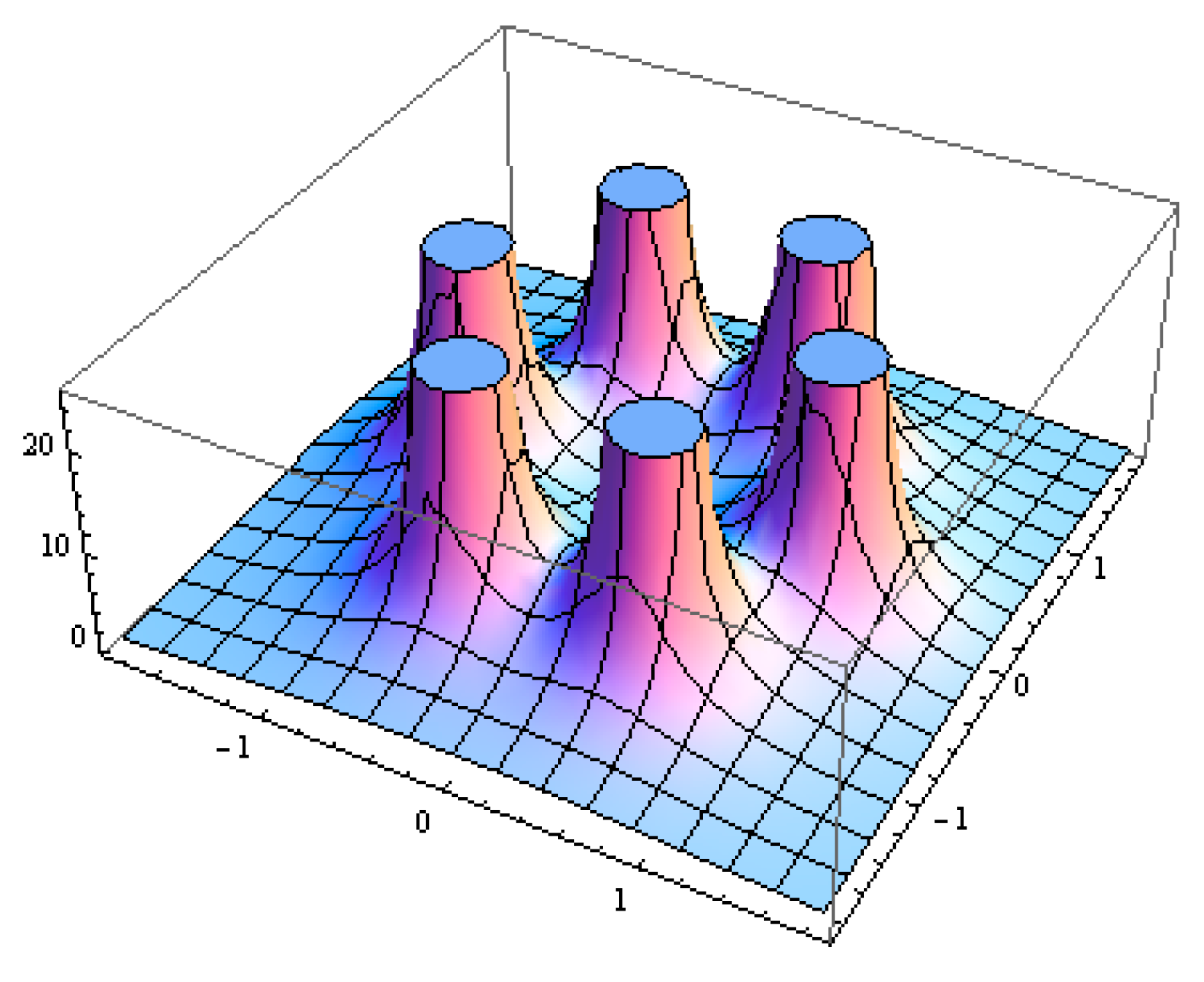
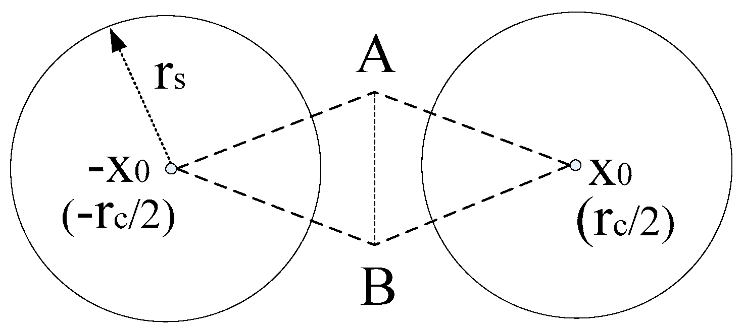
2.2. Information Coverage
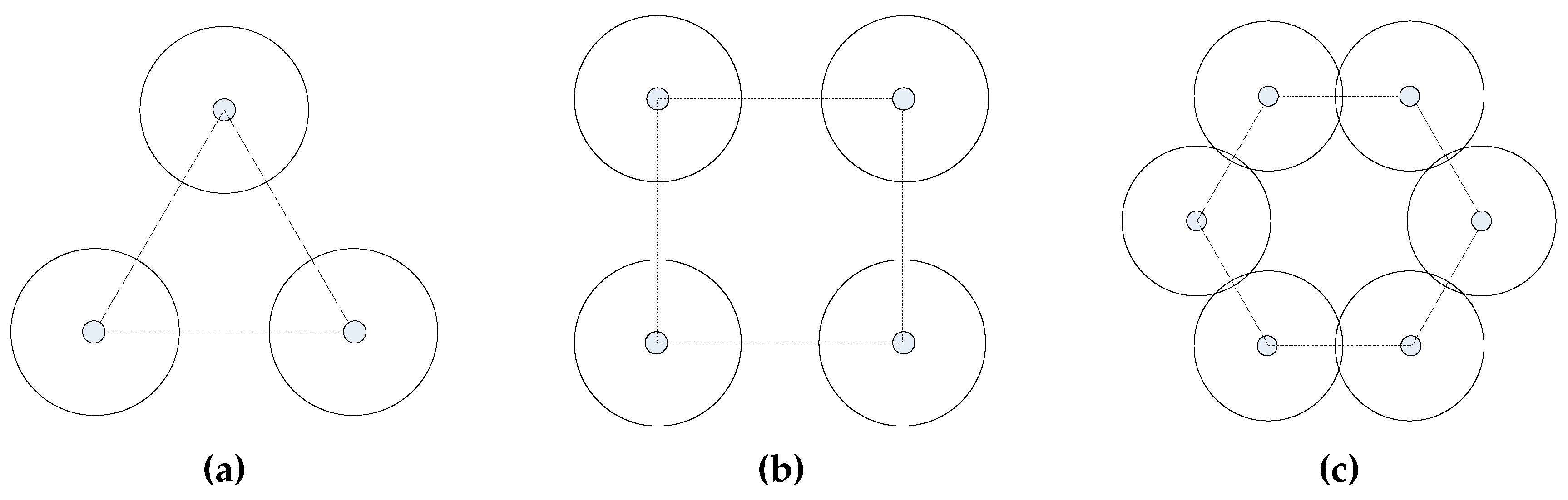
3. Regular Pattern Based Deployment
3.1. Lattice Deployment under Physical Coverage
3.2. Lattice Deployment under Information Coverage
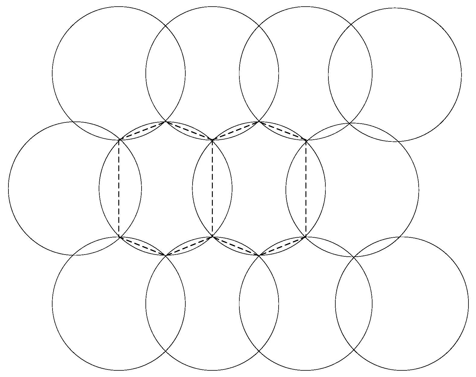
3.3. Dual-Triangular Pattern Deployment
4. Strip-Based Deployment
4.1. Strip-Based Deployment under Physical Coverage
4.2. Strip-Based Deployment Under Information Coverage
5. Discussion and Extension
5.1. Interrelation Between Coverage and Connectivity
5.2. Extension to Information N-Coverage
5.3. Design Issue for Regular Deployment
- (1)
- List out all the issues and factors for your WSN applications, and sort them by importance, doing some quantitative descriptions if possible.
- (2)
- Use the results or analysis method proposed in this paper, while taking the issues and factors into account, to design a deployment scheme for this specific WSN application.
- (3)
- Under constraint conditions, optimize the parameters in order to make the whole network as robust as possible.
6. Numerical Results
6.1. Deployment under Physical Coverage
6.2. Strip-Based Patterns
6.3. Regular Pattern Based Deployments
6.4. Deployment under Infomation Coverage
6.5. Deployment under Different Threshold
6.6. Energy Cost on Messaging
6.7. N-Coverage
7. Conclusions
- (1)
- There is very limited advantage for strip-based deployment in information coverage, since its strategy is collaboration by two sensors, which could not benefit from data fusion more deeply.
- (2)
- Regular deployment in information coverage cannot always outperform it in physical coverage, as value of rc/rs is varied. When the rc/rs is at a very low level, deployment in physical coverage could be a good choice instead, since there is extra cost for data fusion in information coverage.
Acknowledgments
Author Contributions
Conflicts of Interest
Abbreviations
| WSN | Wireless Sensor Networks |
| XSM | Extreme Scale Mote |
| MSE | Mean Squared Error |
| APN | Area Per Node |
References
- Wang, Y.; Zhang, Y.; Liu, J.; Bhandari, R. Coverage, Connectivity, and deployment in wireless sensor networks. In Recent Development in Wireless Sensor and Ad-hoc Networks; Springer: New Delhi, India, 2015; pp. 25–44. [Google Scholar]
- Wang, Y.; Wang, X.; Agrawal, D.P.; Minai, A.A. Impact of Heterogeneity on Coverage and Broadcast Reachability in Wireless Sensor Networks. In Proceedings of 15th International Conference on Computer Communications and Networks, University of Cincinnati, Cincinnati, OH, USA, 9–11 October 2006; pp. 63–67.
- Wang, X.; Xing, G.; Zhang, Y.; Liu, C.; Pless, R.; Gill, G. Integrated coverage and connectivity configuration in wireless sensor networks. In Proceedings of International Conference on Embedded Networked Sensor Systems, Angeles, CA, USA, 5–7 November 2003; pp. 28–39.
- Arora, A.; Ramnath, R.; Ertin, E.; Sinha, P. Exscal: Elements of an extreme scale wireless sensor network. In Proceedings of 11th IEEE International Conference on Embedded and Real-Time Computing Systems and Applications (RTCSA’05), Hong Kong, China, 17–19 August 2005; pp. 102–108.
- Zhang, H.; Hou, J.C. Is Deterministic Deployment Worse than Random Deployment for Wireless Sensor Networks? In Proceedings of the 25th IEEE International Conference on Computer Communications (INFOCOM 2006), Barcelona, Spain, 23–29 April 2006.
- Xing, G.; Wang, X.; Zhang, Y.; Lu, C.; Pless, R.; Gill, C. Integrated Coverage and Connectivity Configuration in Wireless Sensor Networks. ACM Trans. Sens. Netw. 2005, 1, 36–72. [Google Scholar] [CrossRef]
- Iyengar, R.; Kar, K.; Banerjee, S. Low-coordination Topologies for Redundancy in Sensor Networks. In Proceedings of the Sixth ACM Annual International Symposium on Mobile Ad-Hoc Networking and Computing (MobiHoc), Urbana-Champaign, IL, USA, 25–28 May 2005; pp. 332–342.
- Bai, X.; Kumar, S.; Xuan, D.; Yun, Z.; Lai, T.H. Deploying wireless sensors to achieve both coverage and connectivity. In Proceedings of ACM Interational Symposium on Mobile Ad Hoc Networking and Computing (MOBIHOC 2006), Florence, Italy, 22–25 May 2006; pp. 131–142.
- Wang, B.; Wang, W.; Srinivasan, V.; Chua, K.C. Information coverage for wireless sensor networks. IEEE Commun. Lett. 2005, 9, 967–969. [Google Scholar] [CrossRef]
- Wang, B.; Chua, K.C.; Srinivasan, V.; Wang, W. Information Coverage in Randomly Deployed Wireless Sensor Networks. IEEE Trans. Wirel. Commun. 2007, 6, 2994–3004. [Google Scholar] [CrossRef]
- Wang, B. Coverage problems in sensor networks: A survey. ACM Computing Surv. 2011, 43. [Google Scholar] [CrossRef]
- Tian, Y.; Zhang, S.F.; Wang, Y. A Distributed Protocol for Ensuring Both Probabilistic Coverage and Connectivity of High Density Wireless Sensor Networks. In Proceedings of the 2008 IEEE Wireless Communications and Networking Conference, Las Vegas, NV, USA, 31 March–1 April 2008.
- Tsai, Y.R. Sensing Coverage for Randomly Distributed Wireless Sensor Networks in Shadowed Environments. IEEE Trans. Veh. Technol. 2008, 57, 288–291. [Google Scholar]
- Yang, G.; Shukla, V.; Qiao, D. Analytical Study of Collaborative Information Coverage for Object Detection in Sensor Networks. In Proceedings of the 2008 5th Annual IEEE Communications Society Conference on Sensor, Mesh and Ad Hoc Communications and Networks, San Francisco, CA, USA, 16–20 June 2008; pp. 144–152.
- Yang, G.; Qiao, D. Barrier Information Coverage with Wireless Sensors. In Proceedings of the IEEE INFOCOM 2009, Rio de Janeiro, Brazil, 19–25 April 2009; pp. 918–926.
- Li, F.; Deng, K.; Meng, F. Coverage in Wireless Sensor Network Based on Probabilistic Sensing Model. In Proceedings of the 2015 International Conference (AMMIS2015), Nanjing, China, 19–20 June 2015; pp. 527–533.
- Xiang, Y.; Xuan, Z.; Tang, M. 3D space detection and coverage of wireless sensor network based on spatial correlation. J. Netw. Comput. Appl. 2015, 61, 93–101. [Google Scholar] [CrossRef]
- Naranjo, P.G.V.; Shojafar, M.; Mostafaei, H.; Pooranian, Z.; Baccarelli, E. P-SEP: A prolong stable election routing algorithm for energy-limited heterogeneous fog-supported wireless sensor networks. J. Supercomput. 2016. [Google Scholar] [CrossRef]
- Zalyubovskiy, V.; Erzin, A.; Astrakov, S.; Choo, H. Energy-efficient Area Coverage by Sensors with Adjustable Ranges. Sensors 2009, 9, 2446–2460. [Google Scholar] [CrossRef] [PubMed]
- Abbas, W.; Koutsoukos, X. Efficient Complete Coverage through Heterogeneous Sensing Nodes. IEEE Wirel. Commun. Lett. 2015, 4, 14–17. [Google Scholar] [CrossRef]
- Ahmadi, A.; Shojafar, M.; Hajeforosh, S.F.; Dehghan, M.; Singhal, M. An efficient routing algorithm to preserve, k-coverage in wireless sensor networks. J. Supercomput. 2013, 68, 599–623. [Google Scholar] [CrossRef]
- Li, W.X.; Ma, Y.J. On the deployment of wireless sensor networks with regular topology patterns. In Proceedings of International Conference on Web Information Systems and Mining, Chengdu, China, 26–28 October, 2012; pp. 150–158.
- Kim, Y.H.; Kim, C.M.; Yang, D.S.; Oh, Y. Regular sensor deployment patterns for p-coverage and q-connectivity in wireless sensor networks. In Proceedings of the International Conference on Information Network. IEEE Computer Society, Wuhan, China, 1–3 February 2012; pp. 290–295.
- Birjandi, P.A.; Kulik, L.; Tanin, E. K-coverage in regular deterministic sensor deployments. In Proceedings of the IEEE Eighth International Conference on Intelligent Sensors, Melbourne, Australia, 2–5 April 2013; pp. 521–526.
- Hefeeda, M.; Ahmadi, H. Energy-Efficient Protocol for Deterministic and Probabilistic Coverage in Sensor Networks. IEEE Trans. Parallel Distrib. Syst. 2009, 21, 579–593. [Google Scholar] [CrossRef]
- Liu, B.; Towsley, D. A study of the coverage of large-scale sensor networks. In Proceedings of the IEEE International Conference on Mobile Ad-Hoc and Sensor Systems, Paris, France, 25–27 October 2004; pp. 475–483.
- Tian, D.; Georganas, N.D. A coverage-preserving node scheduling scheme for large wireless sensor networks. In Proceedings of the First ACM International Workshop on Wireless Sensor Networks and Applications, Atlanta, GA, USA, 28 September 2002; pp. 32–41.
- Shakkottai, S.; Srikant, R.; Shroff, N.B. Unreliable sensor grids: Coverage, connectivity and diameter. Ad Hoc Netw. 2003, 2, 702–716. [Google Scholar]
- Wang, B. Critical Sensor Density. In Coverage Control in Sensor Networks; Springer: London, UK, 2010; pp. 99–119. [Google Scholar]
- Wang, Y.; Agrawal, D.P. Optimizing sensor networks for autonomous unmanned ground vehicles. Proc. SPIE. 2008. [Google Scholar] [CrossRef]
- Tian, D.; Georganas, N.D. Connectivity maintenance and coverage preservation in wireless sensor networks. Ad Hoc Netw. 2005, 3, 744–761. [Google Scholar] [CrossRef]
- Poe, W.Y.; Schmitt, J.B. Node deployment in large wireless sensor networks: Coverage, energy consumption, and worst-case delay. In Proceedings of the Asian Internet Engineering Conference (AINTEC ‘09), Bangkok, Thailand, 18–20 November 2009; pp. 77–84.
- Xing, G.; Tan, R.; Liu, B.; Wang, J.; Jia, X.; Yi, X.W. Data fusion improves the coverage of wireless sensor networks. In Proceedings of the 15th Annual International Conference on Mobile Computing and Networking, Beijing, China, 20–25 September 2009; pp. 157–168.
- Tan, R.; Xing, G.; Liu, B.; Wang, J. Exploiting data fusion to improve the coverage of wireless sensor networks. IEEE/ACM Trans. Netw. 2012, 20, 450–462. [Google Scholar] [CrossRef]
- Smaragdakis, G.; Matta, I.; Bestavros, A. SEP: A stable election protocol for clustered heterogeneous wireless sensor networks. In Proceedings of the 2nd International Workshop on Sensor and Actor Network Protocol and Applications, Boston, MI, USA, 22 August 2004.


| References | Issue | Coverage Model | rc/rs |
|---|---|---|---|
| [1,8] | Connectivity, Coverage | Physical coverage | Variety |
| [3,5,6,7,26,27,28,29,30,31] | Connectivity, Coverage | Physical coverage | Fixed |
| [9,10,11,14] | Connectivity, Coverage | Information coverage | Fixed |
| [12,13] | Connectivity, Coverage | Probabilistic coverage | Fixed |
| [15] | Connectivity, Barrier Coverage | Information coverage | Fixed |
| [16] | Coverage | Probabilistic coverage | Fixed |
| [17] | 3D Coverage | Probabilistic coverage | Fixed |
| [18] | Connectivity, Coverage | Data fusion | Fixed |
| [2,19,20] | Connectivity, Coverage | Heterogeneous disks | Variety |
| [21,22,23,24] | Multiple Connectivity, Multiple Coverage | Physical coverage | Fixed |
| [25] | Connectivity, Coverage | Probabilistic coverage | Fixed |
| [32,33,34] | Connectivity, Coverage | Data fusion | Fixed |
| Operation | Energy Dissipated |
|---|---|
| Transmitter/Receiver Electronics | Eelec = 50 nJ/bit |
| Data Aggregation | EDA = 50 nJ/bit/report |
| Transmit Amplifier | εfs = 50 nJ/bit/report |
© 2016 by the authors; licensee MDPI, Basel, Switzerland. This article is an open access article distributed under the terms and conditions of the Creative Commons Attribution (CC-BY) license (http://creativecommons.org/licenses/by/4.0/).
Share and Cite
Cheng, W.; Li, Y.; Jiang, Y.; Yin, X. Regular Deployment of Wireless Sensors to Achieve Connectivity and Information Coverage. Sensors 2016, 16, 1270. https://doi.org/10.3390/s16081270
Cheng W, Li Y, Jiang Y, Yin X. Regular Deployment of Wireless Sensors to Achieve Connectivity and Information Coverage. Sensors. 2016; 16(8):1270. https://doi.org/10.3390/s16081270
Chicago/Turabian StyleCheng, Wei, Yong Li, Yi Jiang, and Xipeng Yin. 2016. "Regular Deployment of Wireless Sensors to Achieve Connectivity and Information Coverage" Sensors 16, no. 8: 1270. https://doi.org/10.3390/s16081270