Correction of Dynamic Errors of a Gas Sensor Based on a Parametric Method and a Neural Network Technique

Abstract

The paper presents two methods of dynamic error correction applied to transducers used for the measurement of gas concentration. One of them is based on a parametric model of the transducer dynamics, and the second one uses the artificial neural network (ANN) technique. This article describes research of the dynamic properties of the gas concentration measuring transducer with a typical sensor based on tin dioxide. Its response time is about 8 min, which may be not acceptable in many applications. On the basis of these studies, a parametric model of the transducer dynamics and an adequate correction algorithm has been developed. The results obtained in the research of the transducer were also used for learning and testing ANN, which were implemented in the dynamic correction task. Despite the simplicity of the used models, both methods allowed a significant reduction of the transducer’s response time. For the algorithm based on the parametric model the response time was shorter by approximately eight-fold (reduced up to 40–80 s, i.e., about 2–4 sample periods), whereas with the use of an ANN the output signal was practically fixed after a time equal to one sampling period, i.e., 20 s. In addition, the use of ANN has allowed reducing the impact of the transducer dynamic non-linearity on the correction effectiveness.

1. Introduction

Various types of gas sensors have quite a long response time to a step change in gas concentration. At the beginning there is a transient state, which is dominated by the phenomenon of adsorption (or desorption) of gas molecules in the sensitive layer of sensor. At the end the equilibrium is established and the output signal of the transducer reaches a steady value. This transient state can take quite a long time, from a few, to several, minutes. This is due to two reasons: the phenomenon of chemical adsorption in a sensitive layer occurs relatively slowly [1,2,3,4,5,6,7], and often additional filters and screens are used for example for separation of undesirable substances. In many measurement applications such a long time may be unacceptable for industrial and safety systems. The possibilities of shortening the response time by a suitable design of the sensor or applying better materials of the sensing layer are still being examined [8,9,10]. In some cases, measurements are based on the specific use of transient characteristics of the sensor [11,12,13,14].

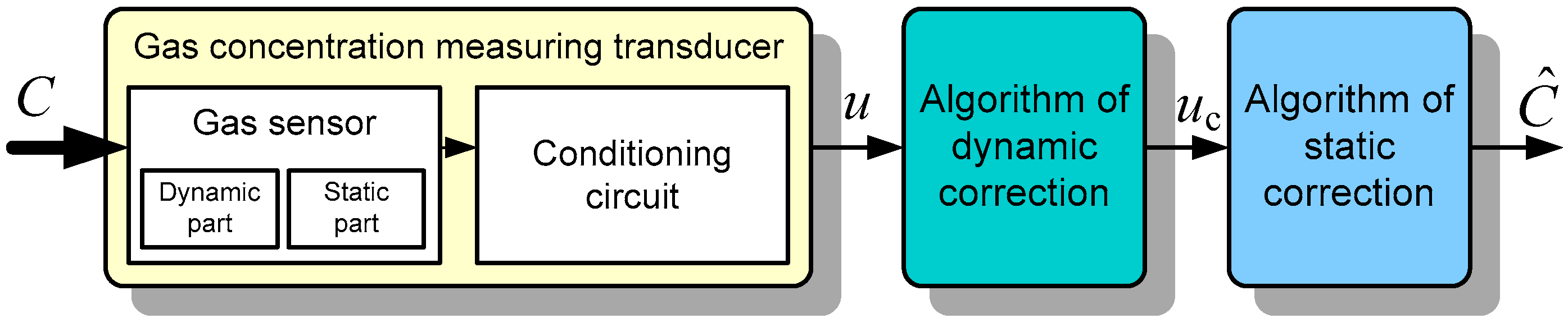
Shortening the response time of the transducer is also possible by the use of a correction procedure implemented by various methods in the next section of the measuring chain. Technical realization of such a correction may be relatively simple and does not necessarily entail the expansion of the measuring chain, because due to the static properties of the sensors (non-linearity, non-selectivity) a procedure of correction of these features is necessary in any case. The basic structure of a transducer to measure gas concentration is shown in Figure 1.

Changes in gas concentration C in the atmosphere surrounding the sensor, due to the phenomenon of adsorption of gas molecules, causes changes of the sensitive layer properties. Consequently, adequate changes of the electrical properties (resistance, permittivity) occur. The sensor can be conventionally divided into two parts. The dynamic part corresponds to a slow adsorption (or desorption) of particles on the surface of the sensitive layer including the possible permeation through the filter, if used. The static part represents the changes of the electrical parameter of the layer as a result of molecule adsorption. Finally, the conditioning circuit produces an output signal u, which depends on the gas concentration. This circuit is treated as a static one. Supplementing the measuring chain by the algorithm of dynamic correction allows the corrected output signal u_c, whose value is fixed after a shorter time, to be obtained. That is the issue discussed in this article in relation to two methods of dynamic correction. The first method is based on knowledge of the structure and parameters of the dynamic model of the sensor and the second one involves using an ANN. Research was carried out for a gas concentration-measuring transducer described in [15] with a solid-state resistive sensor with a SnO₂ sensitive layer (type TGS2442 Figaro, Glenview, IL, USA).

The main motivation of this article is to propose two relatively simple methods to shorten the response time of the low-cost semiconductor gas sensors, which typically have poor dynamic properties.

2. Investigation of the Sensor Dynamics

The analysis of gas sensor dynamic properties carried out in a theoretical manner or by a simulation method [1,2,3] has a significant cognitive meaning. It can be the basis for obtaining a general form (structure) of the dynamic model and, consequently, the dynamic correction algorithm. However, in practice, it is necessary to introduce some measurement results to obtain numerical values of parameters of such a model. In the case of gas sensors it is relatively easy to perform the step response method. 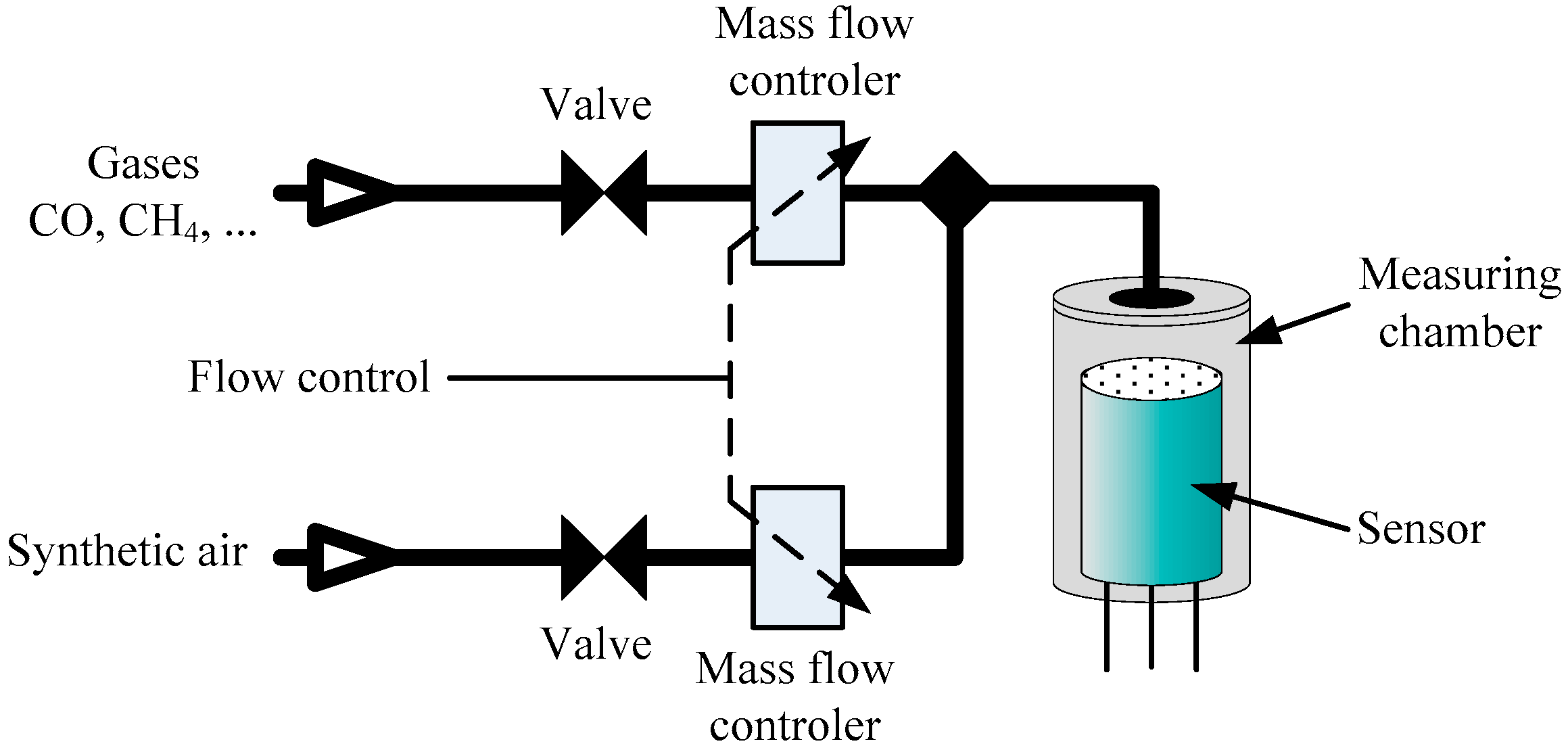Figure 2 shows a scheme of the used measurement system.

Abrupt changes of the gas concentration are obtained by rapid changes of the flow in the channel of the respective constituent gases. Mixing of gases takes place in the inlet channel, so that the concentration in the measuring chamber is already fixed. It is essential that the rise time is sufficiently short. This creates the need for small dimensions of both the inlet channel and the measuring chamber and, at the same time, the use of a high flow rate of the gas mixture. These parameters were chosen in such a way that the rise time of the gas concentration was less than 10 s.

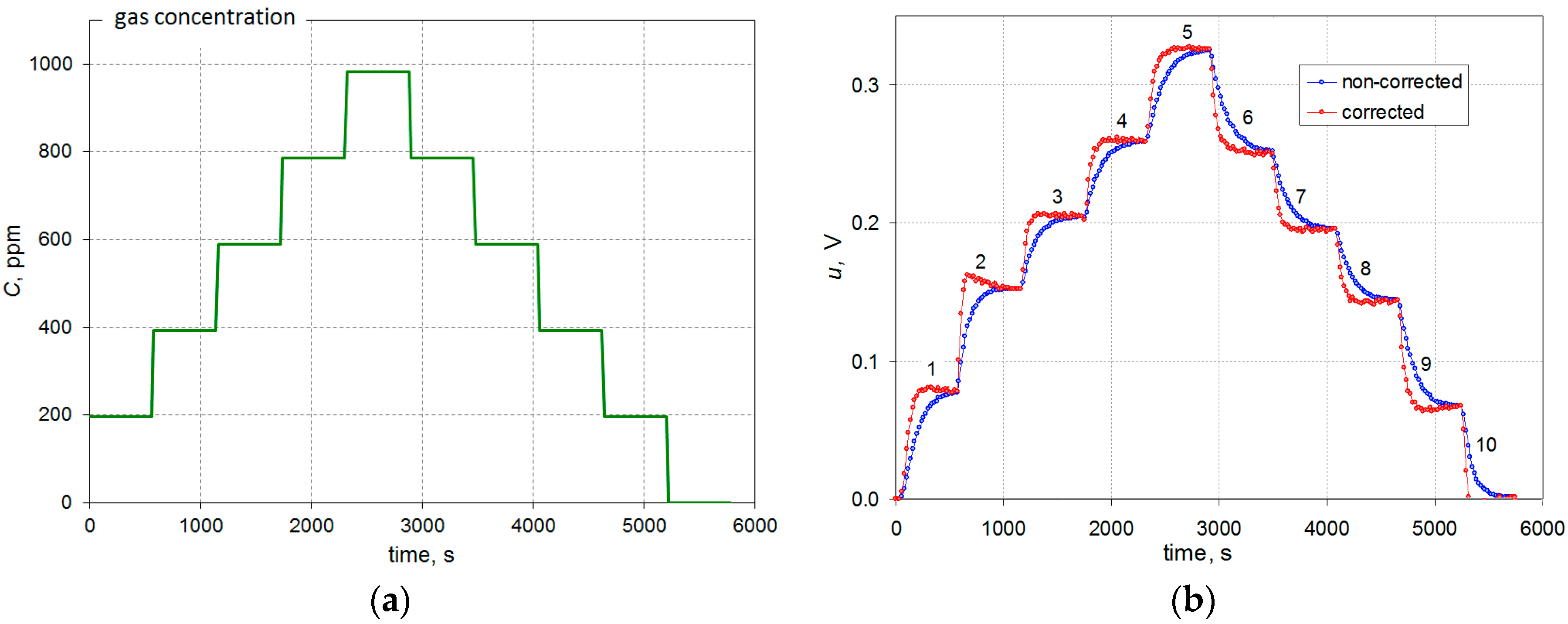
During the tests the gas concentration was changed abruptly as shown in Figure 3a. The resulting changes in the output signal are shown in Figure 3b.

Analysis of the waveforms indicates the inertial nature of the sensor—the output voltage u grows slowly until a steady-state value. Simple, but suitable in this case, are the dynamic models of the first or second order, which may be the basis for the development of the dynamic correction algorithm in the time domain, which can be expressed by the following equations:

$$T\frac{\mathrm{d}u(t)}{\mathrm{d}t}+u(t)=kC(t-T_0)$$

(1)

$$T_1{T}_2\frac{{\mathrm{d}}^{2}u(t)}{\mathrm{d}{t}^2}+\left(T_1+T_2\right)\frac{\mathrm{d}u(t)}{\mathrm{d}t})+u(t)=kC(t)$$

(2)

where C and u are measured gas concentration and output voltage, respectively (see Figure 1), t is time, T, T₁, T₂ (time constants), and T₀ (delay time) are parameters related to the sensor dynamics, and the coefficient k (sensitivity) expresses its static properties. In the presented considerations, determining the sensitivity is not necessary because the subject of the correction are only the dynamic properties and the correction relates to the output voltage of the converter. Problems concerning the correction of the static characteristics of the transducer are discussed in more detail in [16].

As is visible on Figure 3b the constant value of the output signal corresponding to the actual constant value of gas concentration is obtained after more than ten minutes. A dynamic error may be defined as e(t) = u(t) − kC. This error is a function of time and decreases to zero for a steady state. The time interval t_r from a step change in gas concentration until the error e(t_r) is less than 5% of the measuring range, and is called the response time of the measuring transducer.

3. Correction Based on the Dynamic Parametric Model of Sensor (Method 1)

3.1. Identification of the Dynamic Model

In the traditional approach to the development of an algorithm of dynamic correction the structure of the model and values of its parameters must be known. This data can be obtained by the analysis of results of the experiment described above. In spite of the fact that the simplest model of the first order given by the Equation (1) can be useful, the second order model (Equation (2)) was also taken into account for comparison. For the convenience of further consideration these models are expressed by the corresponding equations in the s-domain (using Laplace transform) as the following transfer functions:

$$K_{\text{t1}}(s)=\frac{k}{sT+1}{\mathrm{e}}^{-T_{0}s}\text{ ; }{K}_{\text{t2}}(s)=\frac{k}{\left(s{T}_1+1\right)\left(s{T}_2+1\right)}$$

(3)

where parameters of the model T, T₁, T₂ (time constants), and T₀ (delay time) are determined on the basis of the measurement data (Figure 3b).

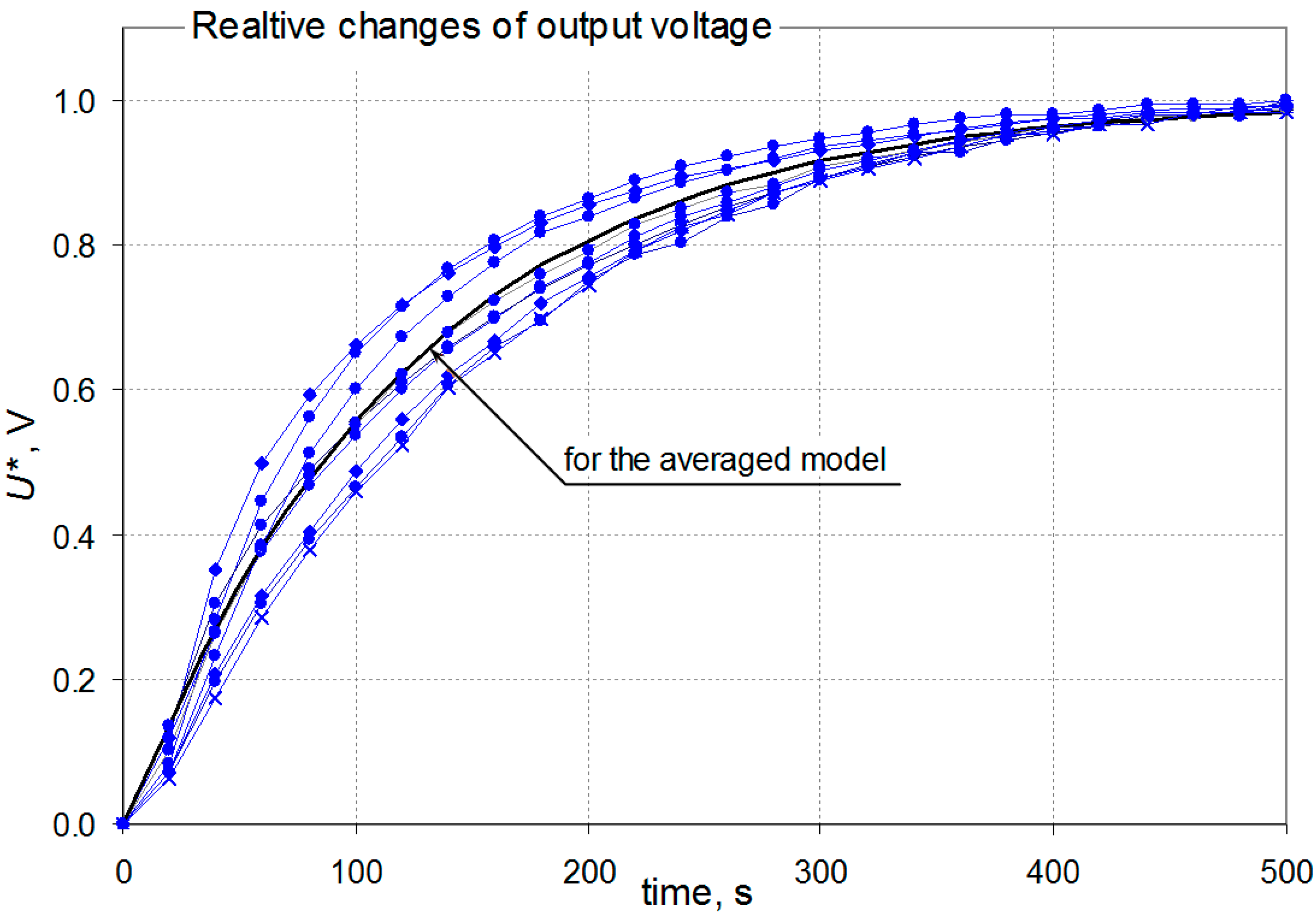
For all phases of the waveform shown in Figure 3b each step response was separated and each one was scaled relative to the steady state values having regard to the direction of the concentration change. The selected set of step responses, including those for the largest and smallest values of the time constants, is shown in Figure 4.

It is evident that the time constants do not have the same values for the concentration changes of various ranges. This means the sensors are dynamically non-linear. The proper implementation of dynamic correction would require taking into account the changes in the dynamic model parameters. However, this study assumed the use of a simplified linear model with the time constant calculated as an average value of the individual time constants for all of the phases. The obtained results of dynamic correction, discussed in Section 3.3, shows that this simplification leads to small dynamic errors. They can be omitted in a first approximation in comparison with errors arising from the imperfect static non-linearity correction and correction of influencing quantities [16]. The averaged time constants of the dynamic models of the sensors were determined based on the average step response—the obtained values are given in

Table 1. A set of parameters of the dynamic models.

Type of Model	Averaged Parameters	Maximum	Minimum
First-order	T = 126.5 s	144.6 s	95.7 s
with delay	t0 = 21.2 s	43.2 s	0.0 s
Second-order	T1 = 126.5 s	144.6 s	95.7 s
	T2 = 24.4 s	40.6 s	0.0 s

.

3.2. Algorithm of the Dynamic Correction

A block diagram shown in Figure 5 illustrates the principle of the proposed dynamic correction method. The dynamic model of the transducer composed of the sensor and a signal conditioner is expressed by the transfer function K_s(s), whereas K_t(s) is a transfer function for the whole system (transducer supplemented with dynamic corrector). For both of them, the same type of model is assumed. In order to shorten the response time by a factor α = (0,…,1), the time constant for the whole transducer can be expressed as αT, so the transfer function of a dynamic corrector can be derived as:

$$K_{\mathrm{c}}(s)=\frac{U_{\mathrm{c}}(s)}{U(s)}=\frac{U_{\mathrm{c}}(s)}{C(s)}\frac{C(s)}{U(s)}=K_{\mathrm{t}}(s)K_{\mathrm{s}}^{\text{-1}}(s)=\frac{k}{sT\mathsf{\alpha }+1}{\left(\frac{k}{sT+1}\right)}^{-1}=\frac{sT+1}{sT\mathsf{\alpha }+1}$$

(4)

where U and U_c denote the values of the voltage before and after dynamic correction (see Figure 1). The same result is obtained when both models (1) and (2) are considered and the reduction concerns the dominant (the greater) time constant. It means that it is T₀ << T₁ or T₂ << T₁ in case (1) or (2), respectively.

After sampling the signal (which is natural in respect of the numerical dynamic correction algorithm) and using the Tustin method to convert models from continuous time into discrete time, a recurrent algorithm of the dynamic corrector can be derived from Equation (4). It has the following form:

$$u_{\mathrm{c}}(n)=\frac{2T+T_{\mathrm{s}}}{2\mathsf{\alpha }T+T_{\mathrm{s}}}u(n)-\frac{2T-T_{\mathrm{s}}}{2\mathsf{\alpha }T+T_{\mathrm{s}}}u(n-1)+\frac{2\mathsf{\alpha }T-T_{\mathrm{s}}}{2\mathsf{\alpha }T+T_{\mathrm{s}}}{u}_{\mathrm{c}}(n-1)$$

(5)

where T_s is the constant sampling period, u(n) and u(n − 1)—output voltage before dynamic correction while u_c(n) and u_c(n − 1) are these after correction in actual n and previous n − 1 cycles of the recurrent calculation.

3.3. Efficiency of Correction

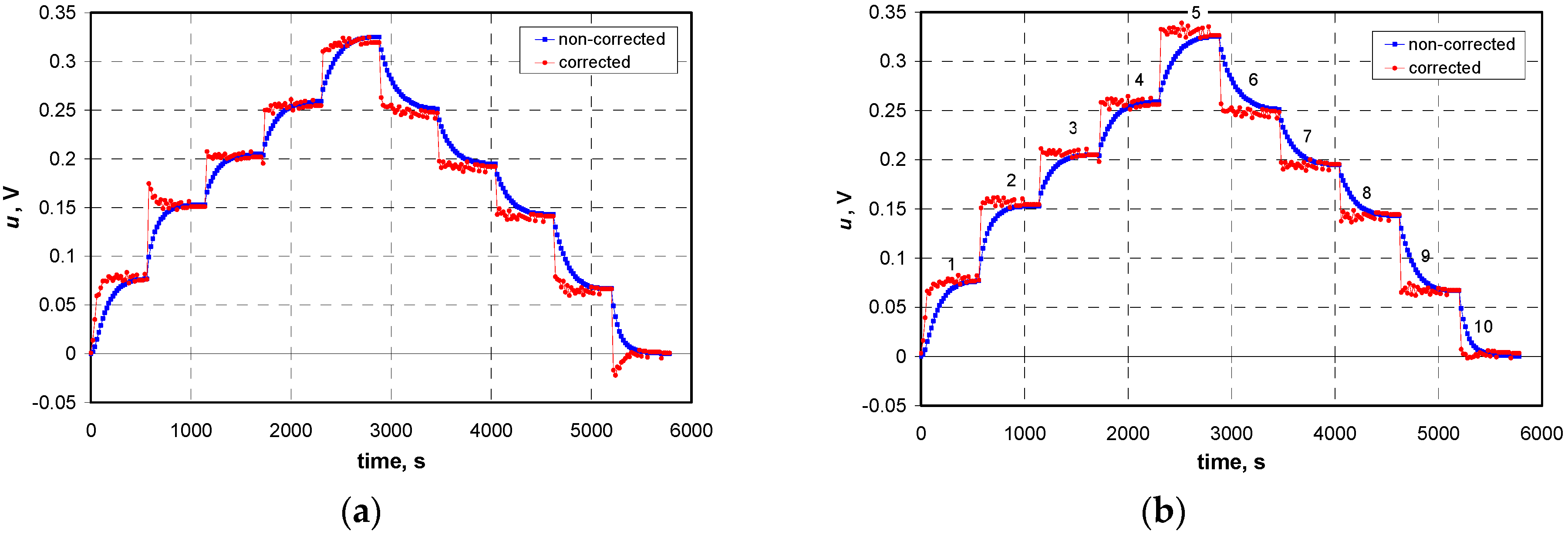
Figure 6 shows an example of application of the dynamic correction algorithm to reconstruct the gas concentration variation in time. The transducer mentioned in the first part was tested. Abrupt changes in concentration followed every 10 min. The parameter α was set equal to 1/4, which means a four-fold reduction of the response time is postulated. This parameter can theoretically be arbitrarily small, but in practice there is no sense to set α less than the quotient of the applicable sampling time T_s and the dominant time constant of the sensor T₁ (in this case approx. 20/120 = 1/6).

The waveform presented in Figure 6 confirms the effectiveness of the above-described dynamic correction method. The response time without correction is eight to ten minutes and after applying the correction in most cases it does not exceed one minute. There are visible small overshoots, mostly for low gas concentrations. This is due to non-ideal matching of the averaged model—the average time constant used in the calculation is not well matched for all ranges of gas concentration. Due to the overshoot effect the algorithm was modified—if the calculated output voltage u_c has negative value, it is set to zero (the last phase in the sequence in Figure 6).

4. Correction Based on an Artificial Neural Network (Method 2)

ANNs are widely used in measurement techniques, which is a consequence of their basic features: the ability to learn and generalize, that is, the ability to generalize the acquired knowledge for new, previously-unknown data. This enables avoiding the necessity of complete and sufficiently precise formal modelling of the analog processing chain, the operation of which can be relatively easily described by “examples”. Especially good approximation properties have feed-forward multilayer neural networks with sigmoidal transfer functions, called Multi Layer Perceptron (MLP) networks or Back Propagation (BP)-type networks [17,18]. These networks are also often used in devices with semiconducting metal oxide-based sensors for detection and concentration estimation of various gases. In many cases, sufficiently good results are obtained with MLP networks with one hidden layer [19,20,21]. In more complex cases generally are sufficient MLP networks with two hidden layers [22,23].

4.1. Real-Time Dynamic Error Correction Algorithm

In general, the dynamic properties of analog transducers are usually modelled by a linear differential equation of the n-th order [24,25,26]. The real-time dynamic correction algorithm can be achieved by presenting this equation as a system of n first order equations in a discrete state space [27,28] and then solving this system due to the input quantity. A detailed description of this algorithm and its neural network implementation is given in [29].

The main disadvantage of the “classic” dynamic correction algorithms is necessary to identify the coefficients of the differential equation describing the dynamics of the sensor. It is required to determine the coefficients of the algorithm which, in general, is a linear combination of these coefficients and subsequent measurement results (e.g.,—Section 3.2).

In the simplest case, the dynamic model of the transducer can be described by a linear first order differential Equation (1) which for T₀ = 0 has the form:

$$T\frac{\mathrm{d}u(t)}{\mathrm{d}t}+u(t)=kC(t)$$

(6)

The real-time dynamic correction algorithm takes the form [29,30,31]:

$$u_{\mathrm{c}}(n)=\frac{1}{\mathsf{\psi }}\left[u(n)-\mathsf{\varphi }u(n-1)\right]$$

(7)

in which u_c(n) is the corrected value of the u(t_n) voltage (Figure 1) at the t_n moment of time, (n = 0, 1, …, N,…) and:

$$\mathsf{\varphi }=\exp \left(-\frac{T_{\mathrm{s}}}{T}\right),\mathsf{\psi }=1-\exp \left(-\frac{T_{\mathrm{s}}}{T}\right)=1-\mathsf{\varphi }$$

(8)

where T_s is the sampling period, and T is the time constant.

As can be seen, the designation of the coefficients $\mathsf{\varphi }$ and ψ requires the identification of the dynamic model time constant T which, in turn, requires a separate process of the model identification. It can be difficult to implement, ineffective, time consuming, and costly, especially for the higher order dynamic model of the sensor. An alternative in such situations is to use an ANN [17,18,32] which “performs” this type of identification in the learning process.

4.2. Neural Network Implementation of the Real-Time Dynamic Error Correction

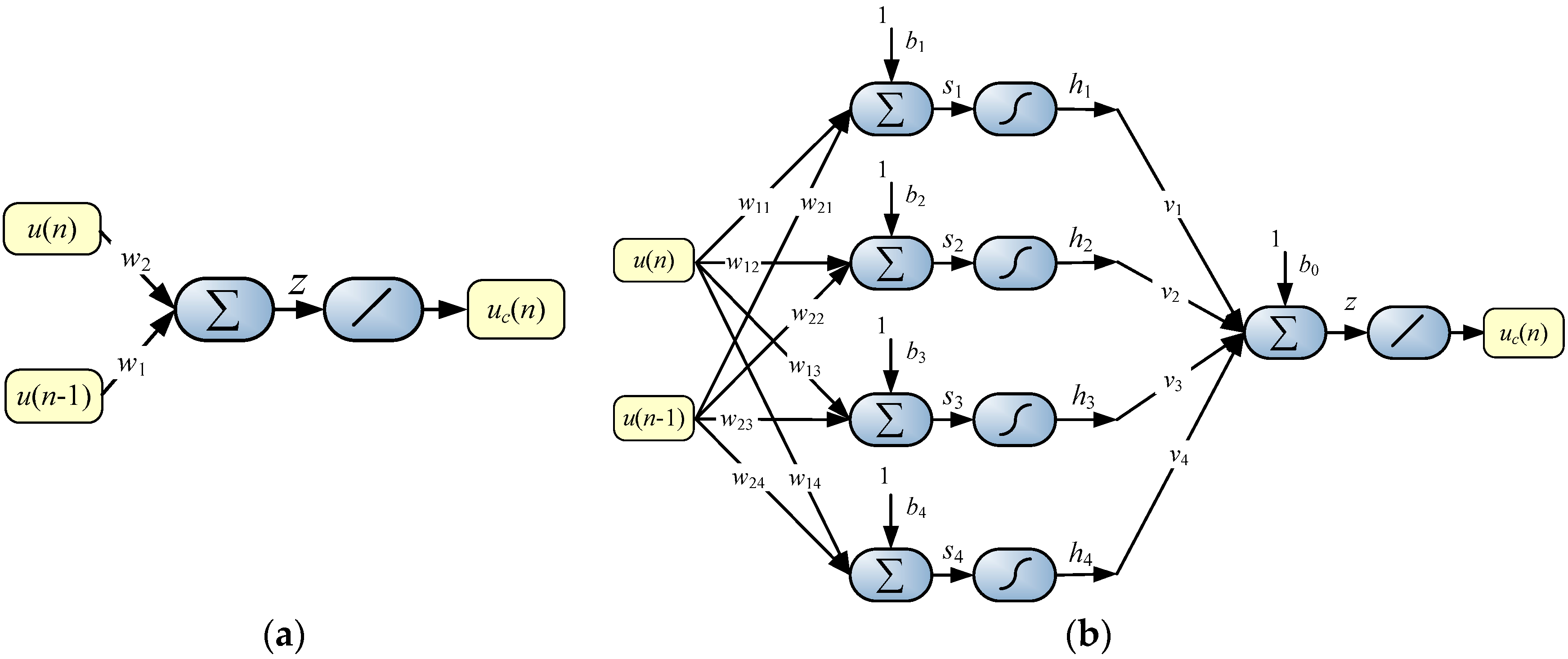
Presenting Equation (7) in the form:

$$u_c(n)=w_{1}u(n-1)+w_{2}u(n)$$

(9)

where $w_1=-\frac{\mathsf{\varphi }}{\mathsf{\psi }}$ and $w_2=\frac{1}{\mathsf{\psi }}$, processing of the linear neuron shown in Figure 7a (u_c(n) = z for linear transfer function) is obtained. In the ideal case, when the sensor is described by a linear first order differential Equation (6) and the measurement results are free of errors, the result of dynamic correction is achieved after a time equal to the sampling period T_s. It can be concluded that the linear neuron during the learning process performs indirect identification of the time constant T.

For the practical verification of the dynamic correction effectiveness implemented by a single linear neuron, the learning process was carried out. This process uses the same dataset as for identification of the dynamic model of the sensor described in Section 3.1. The results of the dynamic correction for the test data are presented in Section 4.3.

In order to take account of the dynamic non-linearity of the sensor, the neural network was expanded by a hidden layer with the sigmoidal [17,18] transfer functions (became an MLP-type neural network). During the research, the ANNs were tested with the number of hidden neurons from 2 to 16, which has shown that in a given case four neurons in the hidden layer are sufficient, so the ANN has the 2-4-1 structure illustrated in Figure 7b. Increasing the number of neurons in the hidden layer or increasing the number of layers did not result in a significant correction improvement.

According to Figure 7b, processing equations of the ANN are as follows:

$$s_i=w_{1i}u(n)+w_{2i}u(n-1)+b_{i}fori=1,\mathrm{...4}$$

(10)

$$h_i=\frac{1}{1+\exp (-s_i)}fori=1,\mathrm{...4}$$

(11)

and:

$$u_c(n)=z={\displaystyle \sum _{j=1}^{j=4}{v}_j{h}_j+b_0}$$

(12)

where w_ji, v_j are weights, and b_j, b₀ are biases of the individual neurons.

4.3. Efficiency of the Correction Performed by ANN

Figure 8a shows the results of dynamic correction implemented by a single linear neuron (Figure 7a). There are correction errors resulting from the assumption of the first order linear model to describe the dynamics of the sensor and random errors resulting from the quantization process additionally increased by the correction algorithm. Dynamic correction errors resulting from the quantization process can be reduced by increasing the resolution of an A/D converter [29] and/or by increasing the sampling period T_s [33].

In turn, Figure 8b illustrates the results of the dynamic correction implemented by the ANN with a 2-4-1 structure (Figure 7b). It can be seen that the addition of a hidden layer improved the dynamic correction quality compared to a single linear neuron. However, the effect of the random error amplification can still be seen. In the cases where errors will exceed the limit values, a variety of filtering or smoothing algorithms can be used [34,35,36].

5. Conclusions

Despite the simplicity of the applied dynamic models for the gas sensor, the dynamic correction algorithms derived from them are very effective—the transducer response time was significantly reduced.

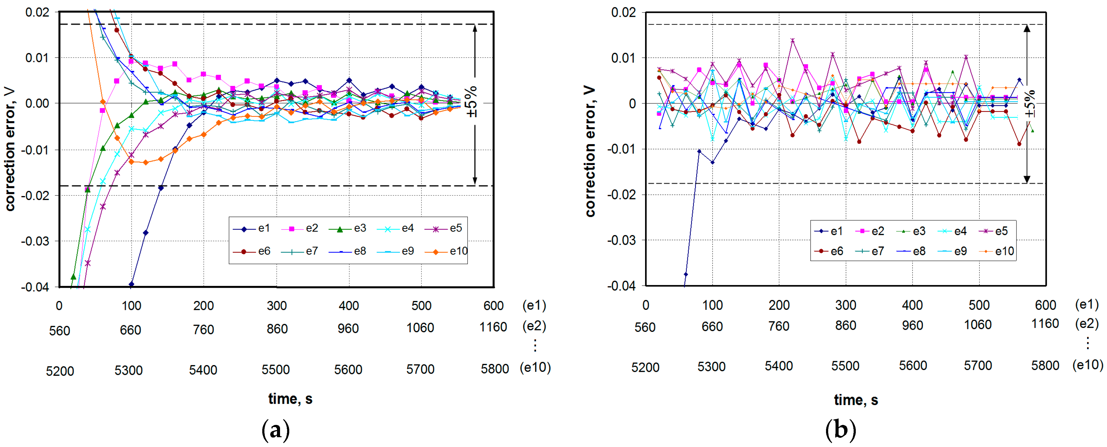
For a more detailed evaluation of the effectiveness of the proposed dynamic correction methods, an dynamic error e(t) has been defined as the difference between the voltage value obtained as a result of the correction u_c(t) and the voltage value in a steady state, which corresponds to the measured gas concentration. Such calculated error values for the two described methods are shown in Figure 9. These methods were compared taking into account three main aspects: the degree of shortening the response time, the impact of the sensor dynamic non-linearity and the impact of random errors.

The transducer response time without correction is about 7–8 min. Both methods used for the dynamic correction allow shortening this time significantly. In the case of Method 1, the response time does not exceed 60 s, whereas in the case of Method 2 (ANN), the time is equal to the sampling period (in the conducted studies: 20 s). The exception is the case of a very small concentration (curve labeled “e1” in Figure 9), for which the response time is twice as long in both methods.

Method 1 does not take into account the dynamic non-linearity of the sensor due to the use of the average model. In this case the degree of shortening the response time depends on the range of changes of the gas concentration and varies between 40 and 90 s. However, in Method 2 the dynamic non-linearity of the sensor can be (to some degree) taken into account by extending the network of the hidden layer with non-linear transfer functions. The research showed that a simple 2-4-1 ANN structure allows obtaining a measurement result after time equal to the sampling period, regardless of changes in the concentration range.

However, it should be noted that the ANN-based dynamic error correction is more sensitive to the random errors of input data than the algorithm proposed in Section 3 (Figure 9a vs. Figure 9b). In a situation when the corrected results contain random errors exceeding limit values several actions can be taken to reduce them. The simplest way is to increase the resolution of the A/D converter. There may also be different smoothing algorithms used or the sampling period may be increased. However, in both cases this leads to an increase in the time to obtain the measurement result.

The application of an ANN technique to the dynamic correction has some significant advantages. The most important of them is that it is not necessary to identify neither the dynamic model of the sensor nor calculate the correction algorithm coefficients. This task is performed during the learning process of the neural network. In addition, a very simple structure of the ANN is sufficient for effective correction of the dynamic errors of a gas transducer.

References

- Llobet, E.; Vilanova, X.; Brezmes, J.; Sueiras, J.E.; Alcubilla, R.; Correig, X. Steady-state and transient behavior of thick-film tin oxide sensors in the presence of gas mixtures. J. Electrochem. Soc. 1998, 145, 1772–1779. [Google Scholar] [CrossRef]
- Matsunaga, N.; Sakai, G.; Shimanoe, K.; Yamazoe, N. Formulation of gas diffusion dynamics for thin film semiconductor gas sensor based on simple reaction-diffusion equation. Sens. Actuators B-Chem. 2003, 96, 226–233. [Google Scholar] [CrossRef]
- Guerin, J.; Bendahan, A.; Aguir, K. A dynamic response model for the WO3-based ozone sensors. Sens. Actuators B-Chem. 2008, 128, 462–467. [Google Scholar] [CrossRef]
- Llobet, E.; Vilanova, X.; Brezmes, J.; Lopez, D.; Correig, X. Electrical equivalent models of semiconductor gas sensors using PSpice. Sens. Actuators B-Chem. 2001, 77, 275–280. [Google Scholar] [CrossRef]
- Gutierrez-Osuna, R.; Gutierrez-Galvez, A.; Powar, N. Transient response analysis for temperature-modulated chemoresistors. Sens. Actuators B-Chem. 2003, 93, 57–66. [Google Scholar] [CrossRef]
- Stamenov, P.; Madathil, R.; Coey, J.M.D. Dynamic response of ammonia sensors constructed from polyaniline nanofibre films with varying morphology. Sens. Actuators B-Chem. 2012, 161, 989–999. [Google Scholar] [CrossRef]
- Buck, A.L.; Roberts, M.I.; Overfelt, R.A.; Prorok, B.C.; Crumpler, M.S. Transient response characteristics of electrochemical carbon monoxide sensors. In Proceedings of the 43rd International Conference on Environmental Systems (ICES 2013), Vail, CO, USA, 14–18 July 2013.
- Basu, S.A.; Wang, Y.-H.A.B.; Ghanshyam, C.A.; Kapur, P.A.Q. Fast response time alcohol gas sensor using nanocrystalline F-doped SnO2 films derived via sol-gel method. Bull. Mater. Sci. 2013, 36, 521–533. [Google Scholar] [CrossRef]
- Vander Wal, R.L.; Berger, G.M.; Kulis, M.J.; Hunter, G.W.; Xu, J.C.; Evans, L. Synthesis Methods, Microscopy Characterization and Device Integration of Nanoscale Metal Oxide Semiconductors for Gas Sensing. Sensors 2009, 9, 7866–7902. [Google Scholar] [CrossRef] [PubMed]
- Kanan, S.M.; El-Kadri, O.M.; Abu-Yousef, I.A.; Kanan, M.C. Semiconducting Metal Oxide Based Sensors for Selective Gas Pollutant Detection. Sensors 2009, 9, 8158–8196. [Google Scholar] [CrossRef] [PubMed]
- Sobanski, T.; Modrak, I.; Nitsch, K.; Licznerski, B.W. Application of sensor dynamic response analysis to improve the accuracy of odour-measuring systems. Meas. Sci. Technol. 2006, 17. [Google Scholar] [CrossRef]
- Gajdosik, L. The concentration measurement with SnO2 gas sensor operated in the dynamic regime. Sens. Actuators B-Chem. 2005, 106, 691–699. [Google Scholar]
- Jakubik, W.; Urbanczyk, M. SAW hydrogen sensor with a bilayer structure based on interaction speed. Sens. Actuators B-Chem. 2005, 106, 602–608. [Google Scholar]
- Ngo, K.A.; Lauque, P.; Aguir, K. Identification of toxic gases using steady-state and transient responses of gas sensor array. Sens. Mater. 2006, 18, 251–260. [Google Scholar]
- Urzędniczok, H. Measuring transducer of gas concentration in gas mixture. Prz. Elektrotech. (Electr. Rev.) 2012, 86, 114–117. [Google Scholar]
- Urzędniczok, H. A numerical method of correcting the influence of the additional quantities for nonselective sensors. In Proceedings of the 19th IMEKO TC-4 Symposium “Measurements of Electrical Quantities”, Barcelona, Spain, 18–19 July 2013; pp. 367–371.
- Haykin, S. Neural Networks and Learning Machines, 3rd ed.; Prentice Hall: Ramsey, NJ, USA, 2009. [Google Scholar]
- Gupta, M.; Homma, N.; Jin, L. Static and Dynamic Neural Networks: From Fundamentals to Advanced Theory; John Wiley & Sons, Inc.: New York, NY, USA, 2003. [Google Scholar]
- Zhang, L.; Tian, F. Performance Study of Multilayer Perceptrons in a LowCost Electronic Nose. IEEE Trans. Instrum. Meas. 2014, 63, 1670–1679. [Google Scholar] [CrossRef]
- Srivastava, A.K. Detection of volatile organic compounds (VOCs) using SnO2 gas-sensor array and artificial neural network. Sens. Actuators B-Chem. 2003, 96, 24–37. [Google Scholar] [CrossRef]
- Muckley, E.; Lynch, J.; Kumara, R.; Sumptera, B.; Ivanov, I.N. PEDOT:PSS/QCM-based multimodal humidity and pressure sensor. Sens. Actuators B-Chem. 2016, 236, 91–98. [Google Scholar] [CrossRef]
- Zhang, L.; Tian, F.; Liu, S.; Guo, J.; Hu, B.; Ye, Q.; Dang, L.; Kadri, C.; Feng, J. Chaos based neural network optimization for concentration estimation of indoor air contaminants by an electronic nose. Sens. Actuators A Phys. 2013, 189, 161–167. [Google Scholar] [CrossRef]
- Kouda, S.; Dibi, Z.; Dendouga, A.; Meddour, F.; Barra, S. Optimization of TiO2 and PMAPTAC Concentrations of a Chemical Humidity Sensing Mechanism. Sensors 2009, 9, 7837–7848. [Google Scholar] [CrossRef] [PubMed]
- Fraden, J. Handbook of Modern Sensors; Springer International Publishing: Zug, Switzerland, 2016. [Google Scholar]
- Burns, R.S. Advanced Control Engineering; Butterworth-Heinemann: Saint Louis, MI, USA, 2001. [Google Scholar]
- Bojarska, M.; Jakubiec, J. A method of modelling sampling converter dynamic errors. Metrol. Meas. Syst. 2001, 8, 337–355. [Google Scholar]
- Palm, W.J., III. System Dynamics, 3rd ed.; McGraw-Hill Higher Education: New York, NY, USA, 2013. [Google Scholar]
- Dorf, R.C.; Bishop, R.H. Modern Control Systems, 12th ed.; Prentice Hall: Ramsey, NJ, USA, 2011. [Google Scholar]
- Roj, J. Neural network based real-time correction of transducer dynamic errors. Meas. Sci. Rev. 2013, 13, 286–291. [Google Scholar] [CrossRef]
- Jakubiec, J.; Makowski, P.; Roj, J. Error Model Application in Neural Reconstruction of Nonlinear Sensor Input Signal. IEEE Trans. Instrum. Meas. 2009, 58, 649–656. [Google Scholar] [CrossRef]
- Roj, J.; Urzędniczok, H. Correction of gas sensor dynamic errors by means of neural networks. Meas. Autom. Monit. 2015, 61, 538–541. [Google Scholar]
- Glowacz, A.; Glowacz, A.; Glowacz, Z. Recognition of monochrome thermal images of synchronous motor with the application of quadtree decomposition and backpropagation neural network. Maint. Reliab. 2014, 16, 92–96. [Google Scholar]
- Konopka, K.; Topór-Kamiński, T. Identification of measurement data processing algorithm coefficients presented on selected form of FFT algorithm. Fundamental and Applied Metrology. In Proceedings of the IMEKO XIX World Congress, Lisbon, Portugal, 6–11 September 2009; pp. 2400–2404.
- Orfanidis, S.J. Introduction to Signal Processing; Englewood Cliffs, N.J., Ed.; Prentice Hall: Ramsey, NJ, USA, 1996. [Google Scholar]
- Hamming, R.W. Digital Filters, 3rd ed.; Dover Publications: New York, NY, USA, 1998. [Google Scholar]
- Oppenheim, A.V.; Schafer, R.W. Discrete-Time Signal Processing, 3rd ed.; Prentice-Hall: Ramsey, NJ, USA, 2009. [Google Scholar]
© 2016 by the author; licensee MDPI, Basel, Switzerland. This article is an open access article distributed under the terms and conditions of the Creative Commons Attribution (CC-BY) license (http://creativecommons.org/licenses/by/4.0/).