
System Description and First Application of an FPGA-Based Simultaneous Multi-Frequency Electrical Impedance Tomography


Abstract
:1. Introduction
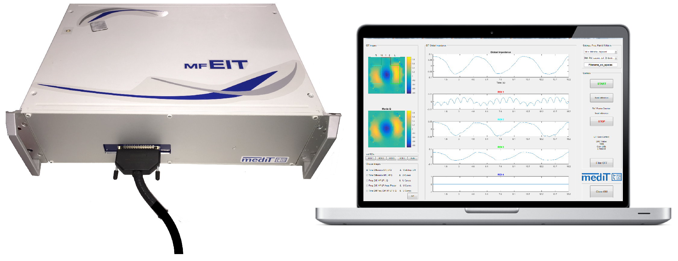
2. System Design
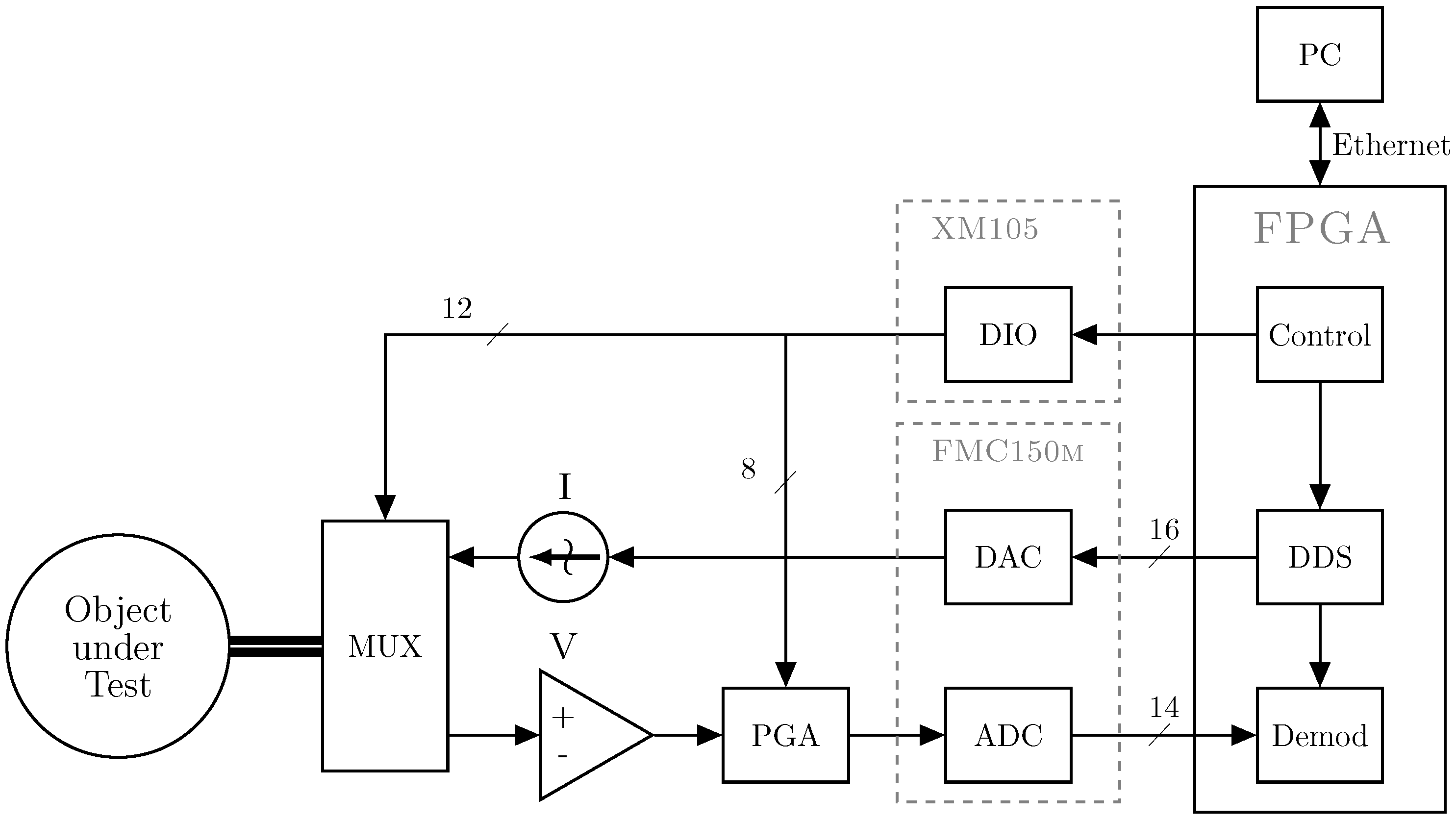
2.1. Main Controller
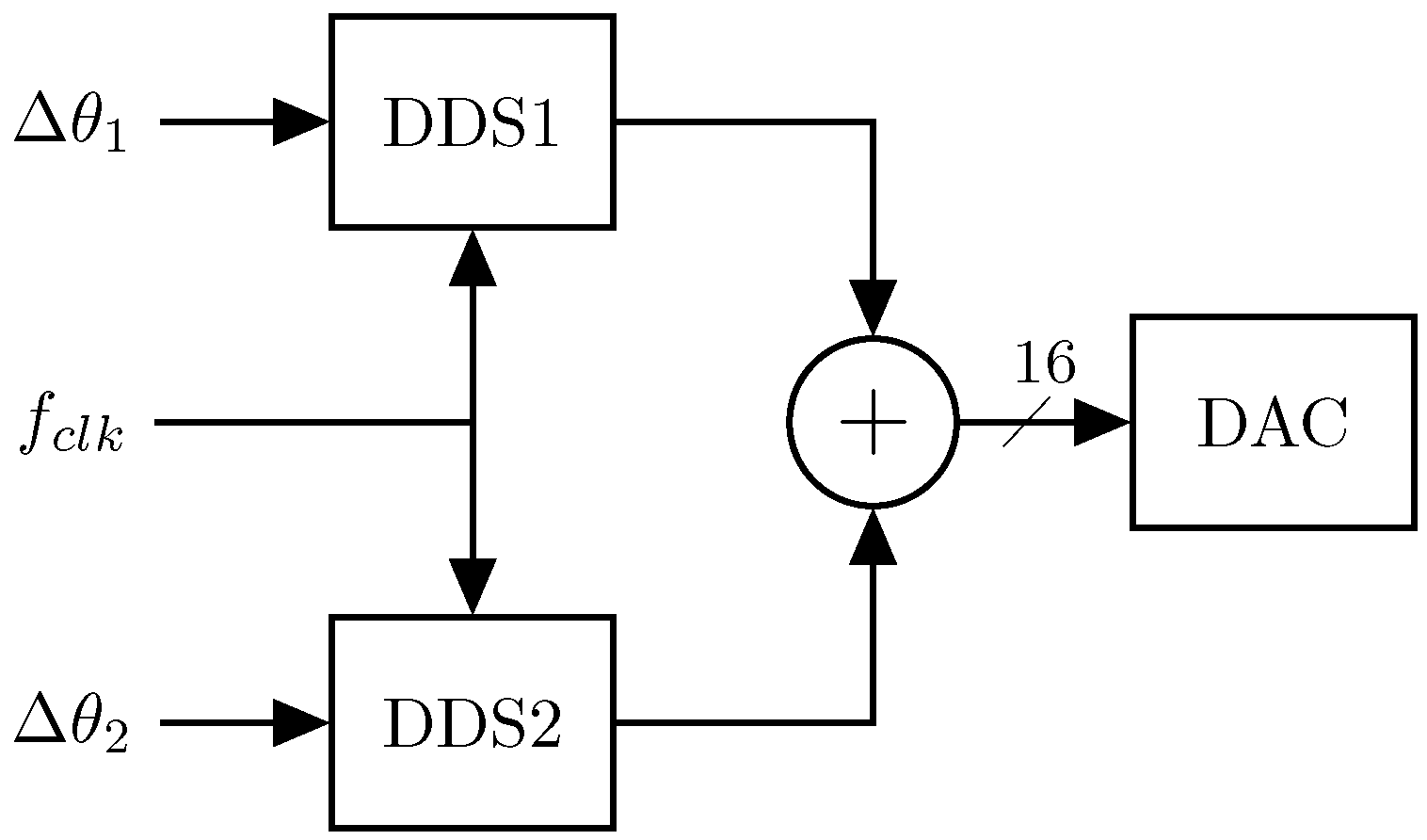
2.2. Signal Generation
- injecting two single currents of different frequencies at two separated electrode pairs simultaneously [19];
Multi-Sine Waveform Generator
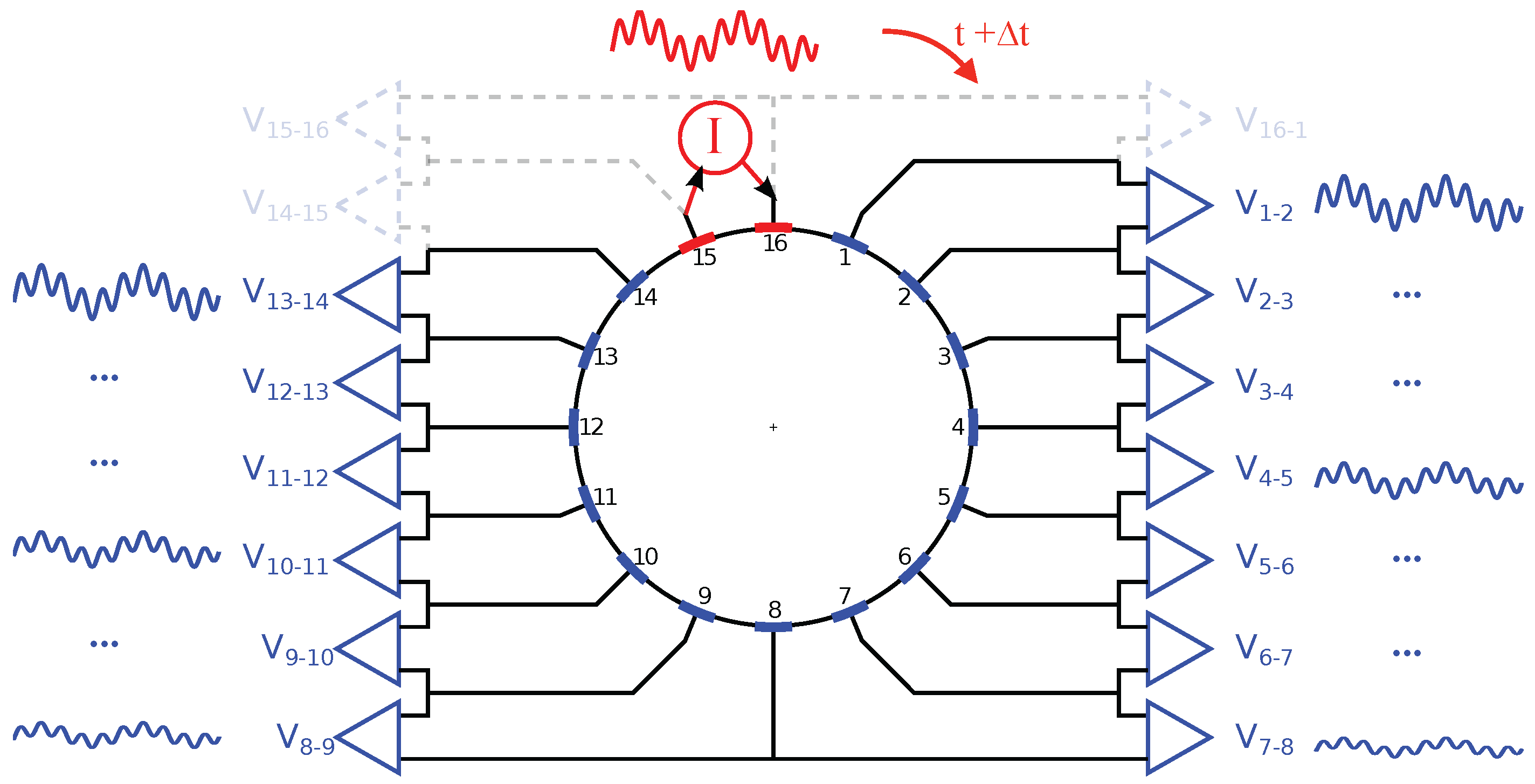
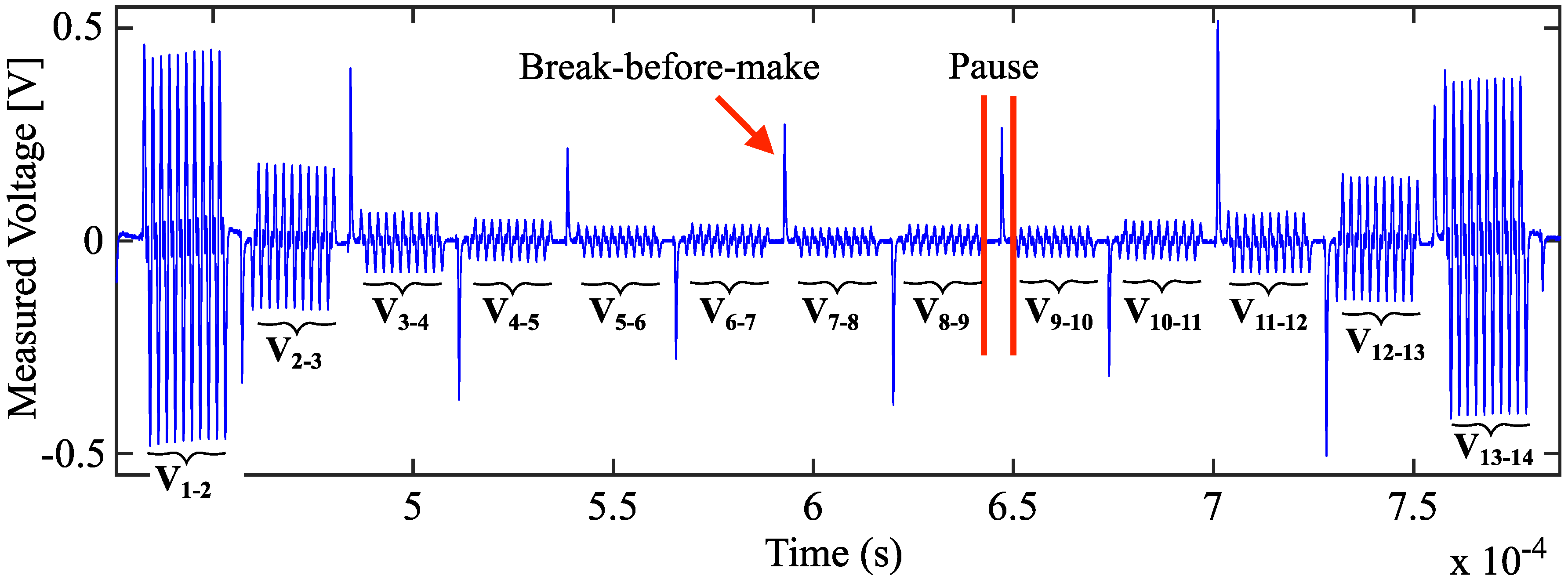
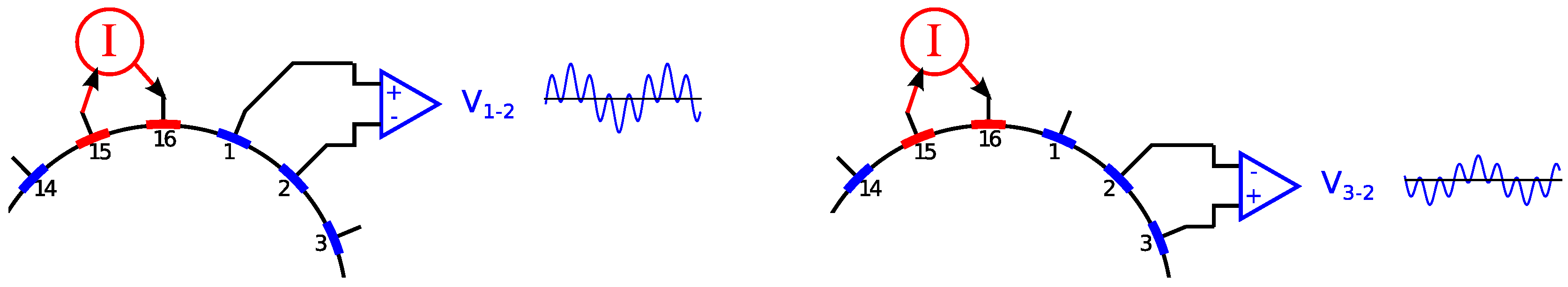
2.3. Electrode Multiplexing
2.4. Data Acquisition and Processing
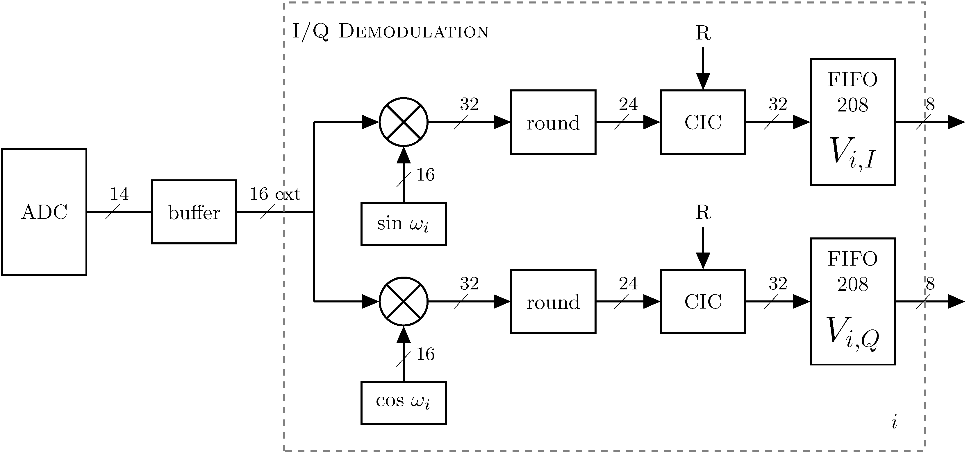
2.4.1. Phase-Sensitive Demodulation
2.4.2. Increasing the Resolution of the ADC-Channel
2.5. Data Transfer
2.5.1. Data Rate
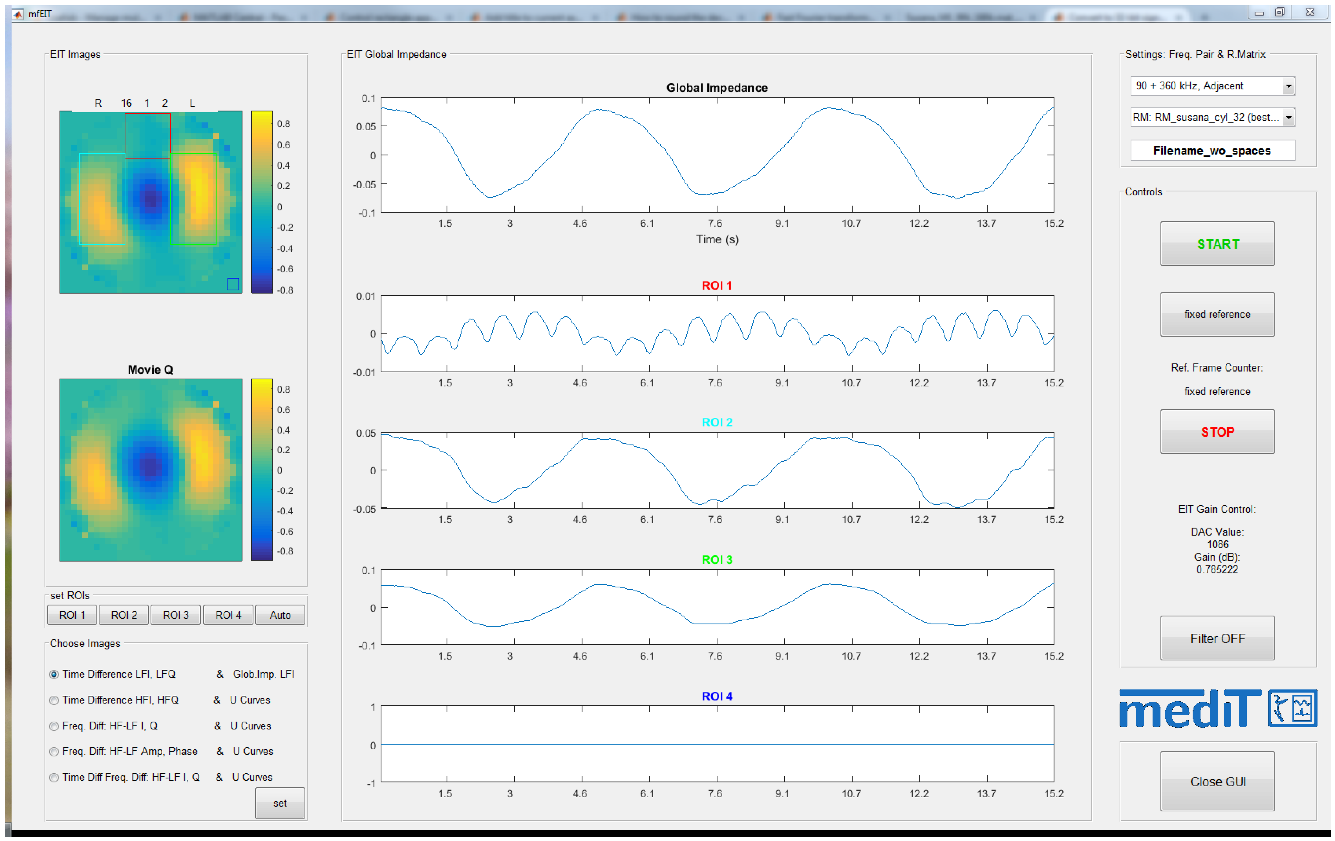
2.5.2. Multi-Frequency EIT Software
3. Measurement Setup
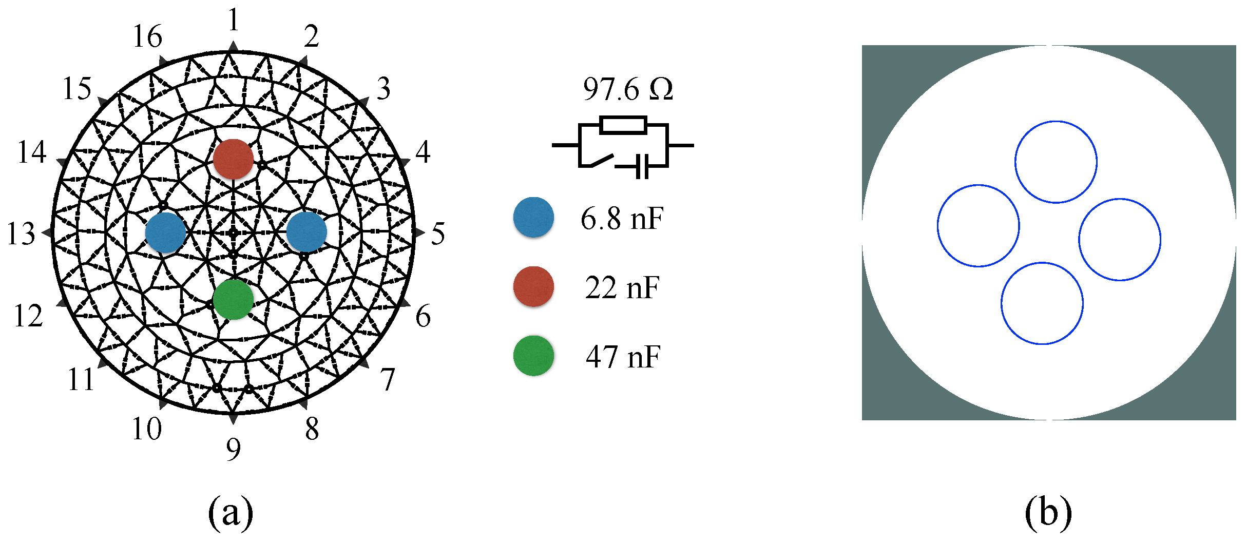
3.1. Resistor/Capacitor Test Unit
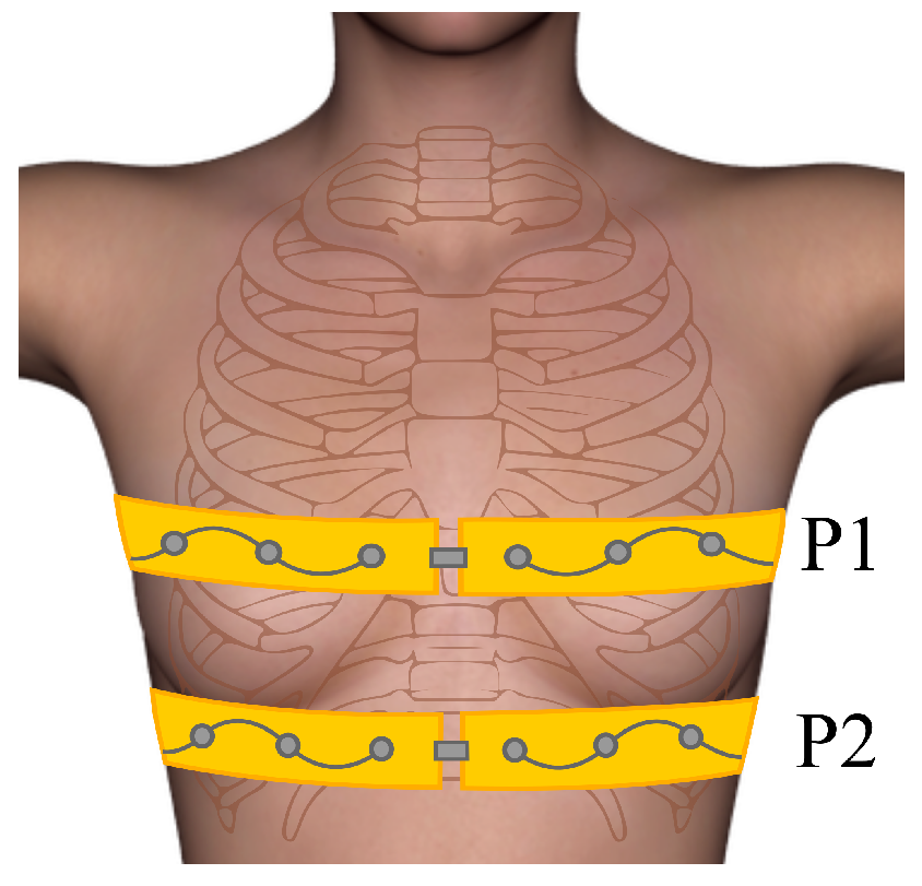
3.2. Human Experiments/Self-Experiment
4. Results
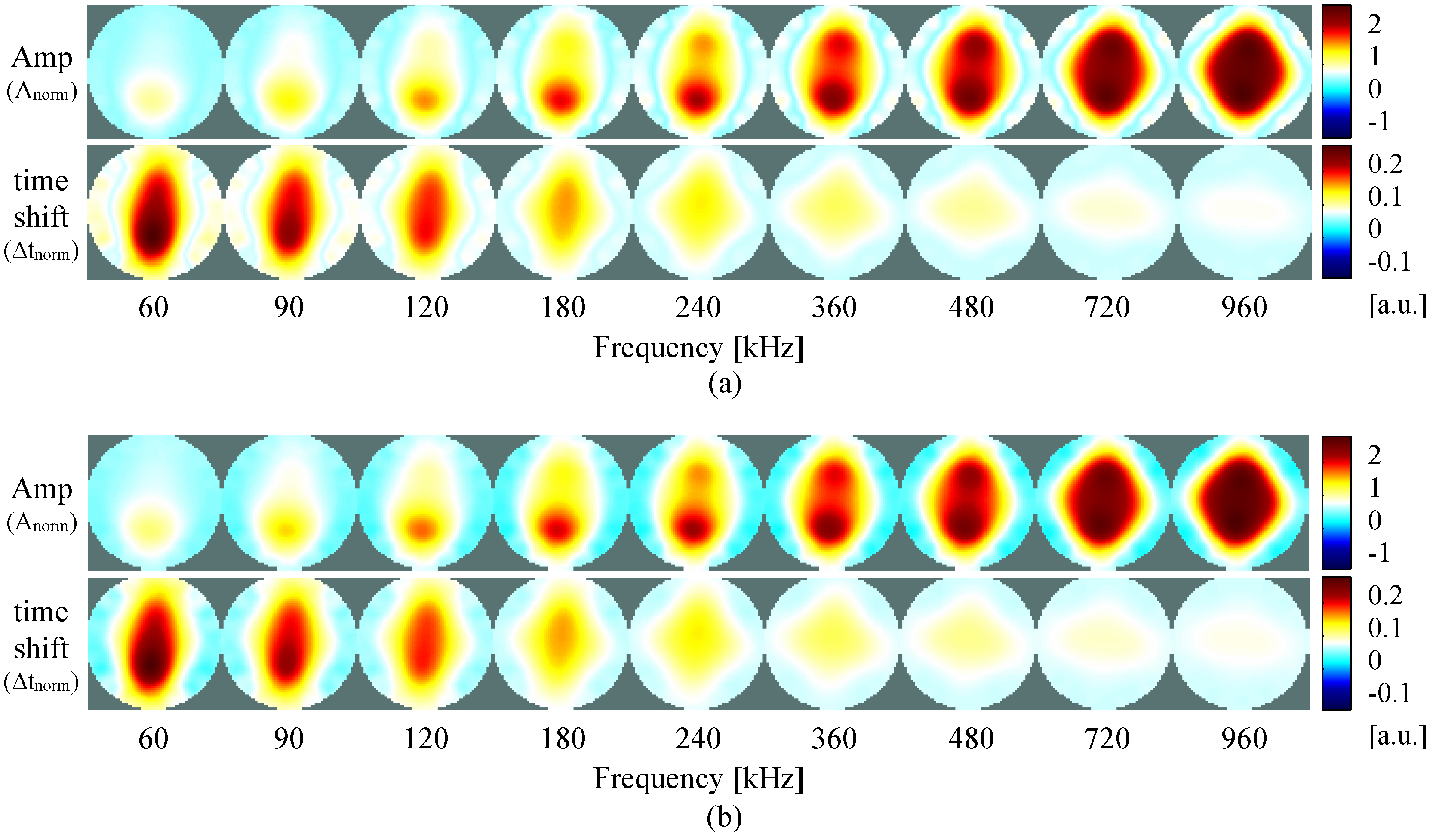
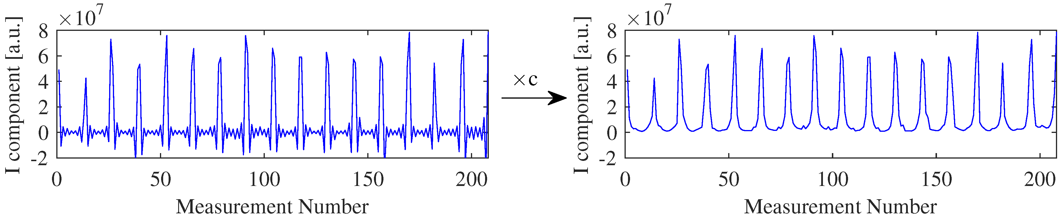
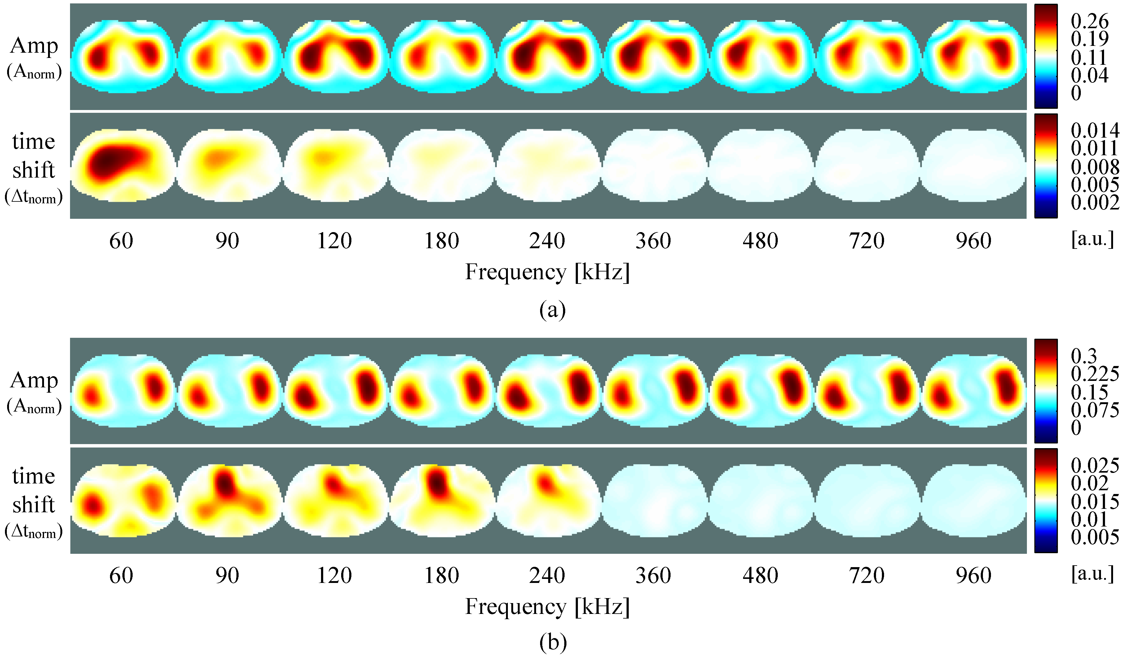
4.1. Resistive/Capacitive Test Unit
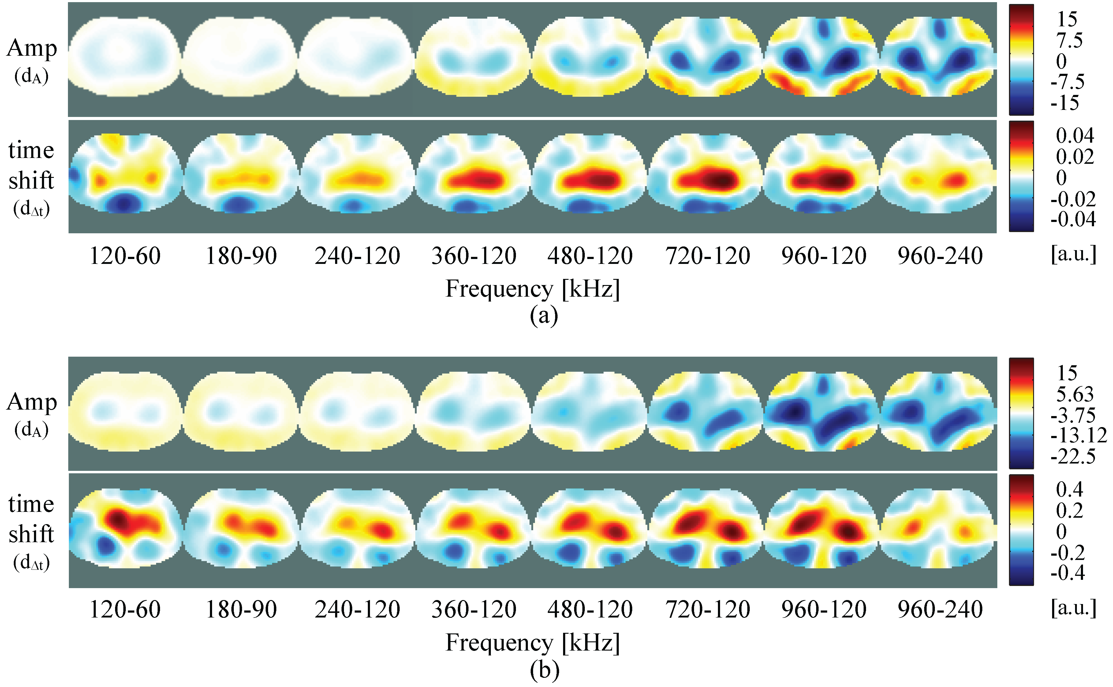
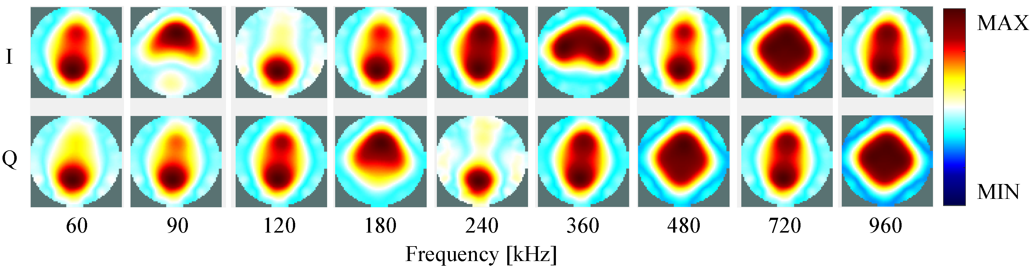
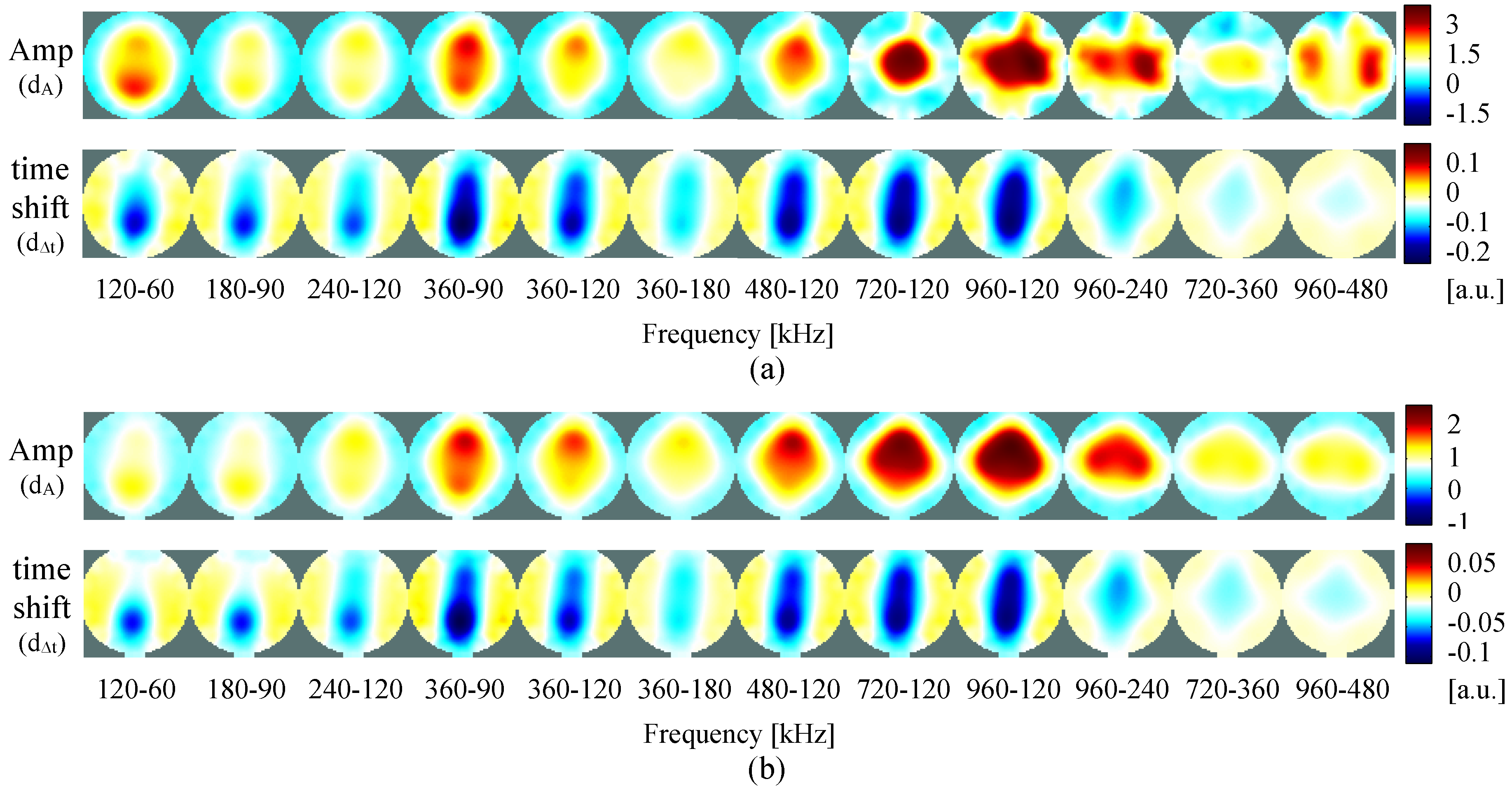
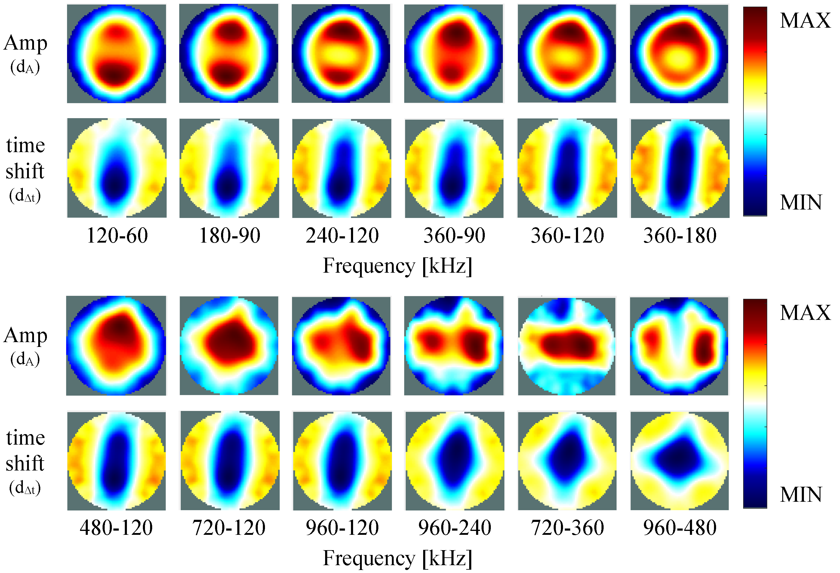
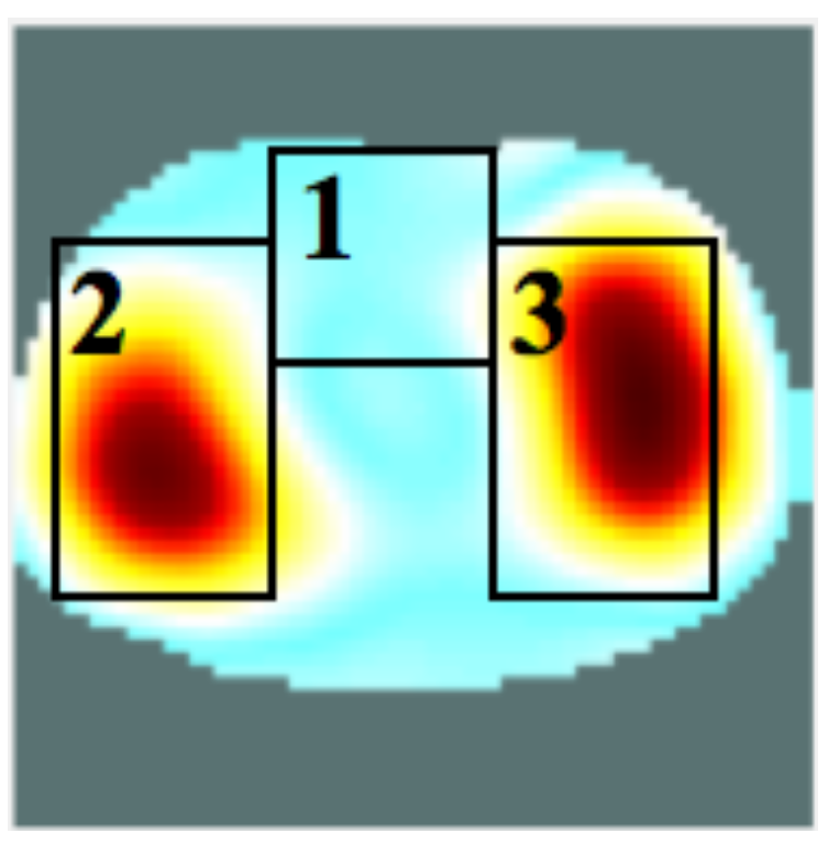
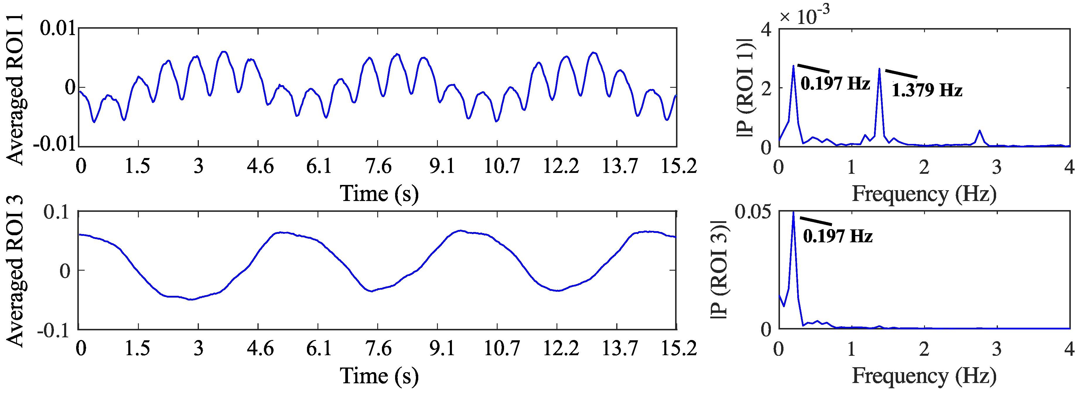
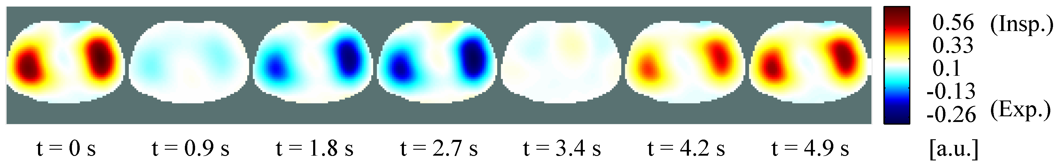
4.2. Self-Experiment
5. Discussion and Conclusions
Supplementary Materials
Acknowledgments

Author Contributions
Conflicts of Interest
References
- Leonhardt, S.; Lachmann, B. Electrical impedance tomography: The holy grail of ventilation and perfusion monitoring? Intensive Care Med. 2012, 38, 1917–1929. [Google Scholar] [CrossRef] [PubMed]
- Bayford, R. Bioimpedance Tomography (Electrical Impedance Tomography). Annu. Rev. Biomed. Eng. 2006, 8, 63–91. [Google Scholar] [CrossRef] [PubMed]
- Cheney, M.; Isaacson, D.; Newell, J.C. Electrical Impedance Tomography. SIAM Rev. 1999, 41, 85–101. [Google Scholar] [CrossRef]
- Brown, B.; Seagar, A. The Sheffield Data Collection System. Clin. Phys. Physiol. Meas. 1987, 8, 91–97. [Google Scholar] [CrossRef] [PubMed]
- Smith, R.; Freeston, I.; Brown, B. A real-time electrical impedance tomography system for clinical use-design and preliminary results. IEEE Trans. Biomed. Eng. 1995, 42, 133–140. [Google Scholar] [CrossRef] [PubMed]
- Gaggero, P.O.; Adler, A.; Brunner, J.; Seitz, P. Electrical impedance tomography system based on active electrodes. Physiol. Meas. 2012, 33, 831–847. [Google Scholar] [CrossRef] [PubMed]
- Wilson, A.J.; Milnes, P.; Waterworth, A.R.; Smallwood, R.H.; Brown, B.H. Mk3.5: A modular, multi-frequency successor to the Mk3a EIS/EIT system. Physiol. Meas. 2001, 22, 49–54. [Google Scholar] [CrossRef] [PubMed]
- Liu, N.; Saulnier, G.; Newell, J.; Kao, T. ACT4: A high-precision, multi-frequency electrical impedance tomography. In Proceedings of the 6th Conference on Biomedical Applications of Electrical Impedance Tomography, London, UK, 22–24 June 2005.
- Adler, A.; Amyot, R.; Guardo, R.; Bates, J.; Berthiaume, Y. Monitoring changes in lung air and liquid volumes with electrical impedance tomography. J. Appl. Physiol. 1997, 83, 1762–1767. [Google Scholar] [PubMed]
- Grimnes, S.; Martinsen, O.G. Bioimpedance and Bioelectricity Basics; Academic: London, UK, 2008. [Google Scholar]
- Kuen, J.; Woo, E.J.; Seo, J.K. Multi-frequency time-difference complex conductivity imaging of canine and human lungs using the KHU Mark1 EIT system. Physiol. Meas. 2009, 30, S149–S164. [Google Scholar] [CrossRef] [PubMed]
- Lee, D.; Wi, H.; Woo, E.; Seo, J. Multi-frequency Time-difference EIT Imaging of Lungs using KHU Mark1. In Proceedings of the 9th International Conference on Electrical Impedance Tomography (EIT 2008), Hanover, NH, USA, 16–18 June 2008.
- Oh, T.I.; Koo, H.; Lee, K.H.; Kim, S.M.; Lee, J.; Kim, S.W.; Seo, J.K.; Woo, E.J. Validation of a multi-frequency electrical impedance tomography (mfEIT) system KHU Mark1: Impedance spectroscopy and time-difference imaging. Physiol. Meas. 2008, 29, 295–307. [Google Scholar] [CrossRef] [PubMed]
- Jun, S.C.; Kuen, J.; Lee, J.; Woo, E.J.; Holder, D.; Seo, J.K. Frequency-difference EIT (fdEIT) using weighted difference and equivalent homogeneous admittivity: validation by simulation and tank experiment. Physiol. Meas. 2009, 30, 1087–1099. [Google Scholar] [CrossRef] [PubMed]
- Ahn, S.; Jun, S.C.; Seo, J.K.; Lee, J.; Woo, E.J.; Holder, D. Frequency-difference electrical impedance tomography: Phantom imaging experiments. J. Phys. Conf. Ser. 2010, 224, 012152. [Google Scholar] [CrossRef]
- Kim, S.M.; Oh, T.I.; Woo, E.J.; Kim, S.W.; Seo, J.K. Time- and Frequency-difference Imaging using KHU Mark1 EIT System. In Proceedings of the 13th International Conference on Electrical Bioimpedance and the 8th Conference on Electrical Impedance Tomography: ICEBI 2007, Graz, Austria, 29 August–2 September 2007; pp. 340–343.
- Sohal, H.; Wi, H.; McEwan, A.L.; Woo, E.J.; Oh, T.I. Electrical impedance imaging system using FPGAs for flexibility and interoperability. Biomed. Eng. Online 2014, 13. [Google Scholar] [CrossRef] [PubMed]
- McEwan, A.; Cusick, G.; Holder, D.S. A review of errors in multi-frequency EIT instrumentation. Physiol. Meas. 2007, 28, S197–S215. [Google Scholar] [CrossRef] [PubMed]
- Wi, H.; Yoo, P.; Oh, T.; Woo, E. Cascaded multi-channel EIT system with fast data acquisition by frequency-division and space-division multiplexing. In Proceedings of the 12th International Conference in Electrical Impedance Tomography (EIT 2011), Bath, UK, 4–6 May 2011.
- Seo, J.K.; Lee, J.; Kim, S.W.; Zribi, H.; Woo, E.J. Frequency-difference electrical impedance tomography (fdEIT): Algorithm development and feasibility study. Physiol. Meas. 2008, 29, 929–944. [Google Scholar] [CrossRef] [PubMed]
- Liu, N. ACT4: A High-Precision, Multi-Frequency Electrical Impedance Tomograph; ProQuest: Ann Arbor, MI, USA, 2007. [Google Scholar]
- Kusche, R.; Malhotra, A.; Ryschka, M.; Ardelt, G.; Klimach, P.; Kaufmann, S. A FPGA-Based Broadband EIT System for Complex Bioimpedance Measurements—Design and Performance Estimation. Electronics 2015, 4, 507–525. [Google Scholar] [CrossRef]
- Nahvi, M.; Hoyle, B.S. Wideband electrical impedance tomography. Meas. Sci. Technol. 2008, 19, 094011. [Google Scholar] [CrossRef]
- Kim, S.; Lee, E.J.; Woo, E.J.; Seo, J.K. Asymptotic analysis of the membrane structure to sensitivity of frequency-difference electrical impedance tomography. Inverse Probl. 2012, 28, 075004. [Google Scholar] [CrossRef]
- Romsauerova, A.; McEwan, A.; Holder, D.S. Identification of a suitable current waveform for acute stroke imaging. Physiol. Meas. 2006, 27, S211–S219. [Google Scholar] [CrossRef] [PubMed]
- Xilinx DS794 LogiCORE IP DDS Compiler v5.0. Product specification (March 2011). Available online: http://www.xilinx.com/support/documentation/ip_documentation/ds794_dds_compiler.pdf (accessed on 15 January 2016).
- Vankka, J.; Halonen, K.A. Direct Digital Synthesizers: Theory, Design and Applications; Springer Science & Business Media: Berlin, Germany, 2013; Volume 614. [Google Scholar]
- Malmivuo, J.; Plonsey, R. Bioelectromagnetism—Principles and Applications of Bioelectric and Biomagnetic Fields; Oxford University Press: New York, NY, USA, 1995. [Google Scholar]
- Lathi, B.P. Modern Digital and Analog Communication Systems 3e Osece; Oxford University Press: New York, NY, USA, 1998. [Google Scholar]
- Hogenauer, E. An economical class of digital filters for decimation and interpolation. IEEE Trans. Acoust. Speech Signal Process. 1981, 29, 155–162. [Google Scholar] [CrossRef]
- AVR121: Enhancing ADC resolution by oversampling. Application Note Rev. 8003A-AVR-09/05, Atmel, 2005. Available online: http://www.atmel.com/images/doc8003.pdf (accessed on 15 January 2016).
- Grewal, H. Oversampling the ADC12 for Higher Resolution; Application Report; Texas Instruments Inc.: Dallas, TX, USA, 2006. [Google Scholar]
- Adler, A.; Arnold, J.H.; Bayford, R.; Borsic, A.; Brown, B.; Dixon, P.; Faes, T.J.C.; Frerichs, I.; Gagnon, H.; Gärber, Y.; et al. GREIT: A unified approach to 2D linear EIT reconstruction of lung images. Physiol. Meas. 2009, 30, S35–S55. [Google Scholar] [CrossRef] [PubMed]
- Malbrain, M.L.; Huygh, J.; Dabrowski, W.; de Waele, J.J.; Staelens, A.; Wauters, J. The use of bio-electrical impedance analysis (BIA) to guide fluid management, resuscitation and deresuscitation in critically ill patients: A bench-to-bedside review. Anaesthesiol. Intensive Therapy 2014, 46, 381–391. [Google Scholar] [CrossRef] [PubMed]
- Karsten, J.; Stueber, T.; Voigt, N.; Teschner, E.; Heinze, H. Influence of different electrode belt positions on electrical impedance tomography imaging of regional ventilation: A prospective observational study. Crit. Care 2016, 20. [Google Scholar] [CrossRef] [PubMed]


© 2016 by the authors; licensee MDPI, Basel, Switzerland. This article is an open access article distributed under the terms and conditions of the Creative Commons Attribution (CC-BY) license (http://creativecommons.org/licenses/by/4.0/).
Share and Cite
Aguiar Santos, S.; Robens, A.; Boehm, A.; Leonhardt, S.; Teichmann, D. System Description and First Application of an FPGA-Based Simultaneous Multi-Frequency Electrical Impedance Tomography. Sensors 2016, 16, 1158. https://doi.org/10.3390/s16081158
Aguiar Santos S, Robens A, Boehm A, Leonhardt S, Teichmann D. System Description and First Application of an FPGA-Based Simultaneous Multi-Frequency Electrical Impedance Tomography. Sensors. 2016; 16(8):1158. https://doi.org/10.3390/s16081158
Chicago/Turabian StyleAguiar Santos, Susana, Anne Robens, Anna Boehm, Steffen Leonhardt, and Daniel Teichmann. 2016. "System Description and First Application of an FPGA-Based Simultaneous Multi-Frequency Electrical Impedance Tomography" Sensors 16, no. 8: 1158. https://doi.org/10.3390/s16081158