
A Likelihood-Based SLIC Superpixel Algorithm for SAR Images Using Generalized Gamma Distribution

Abstract
:1. Introduction
2. Standard SLIC Algorithm
- (1)
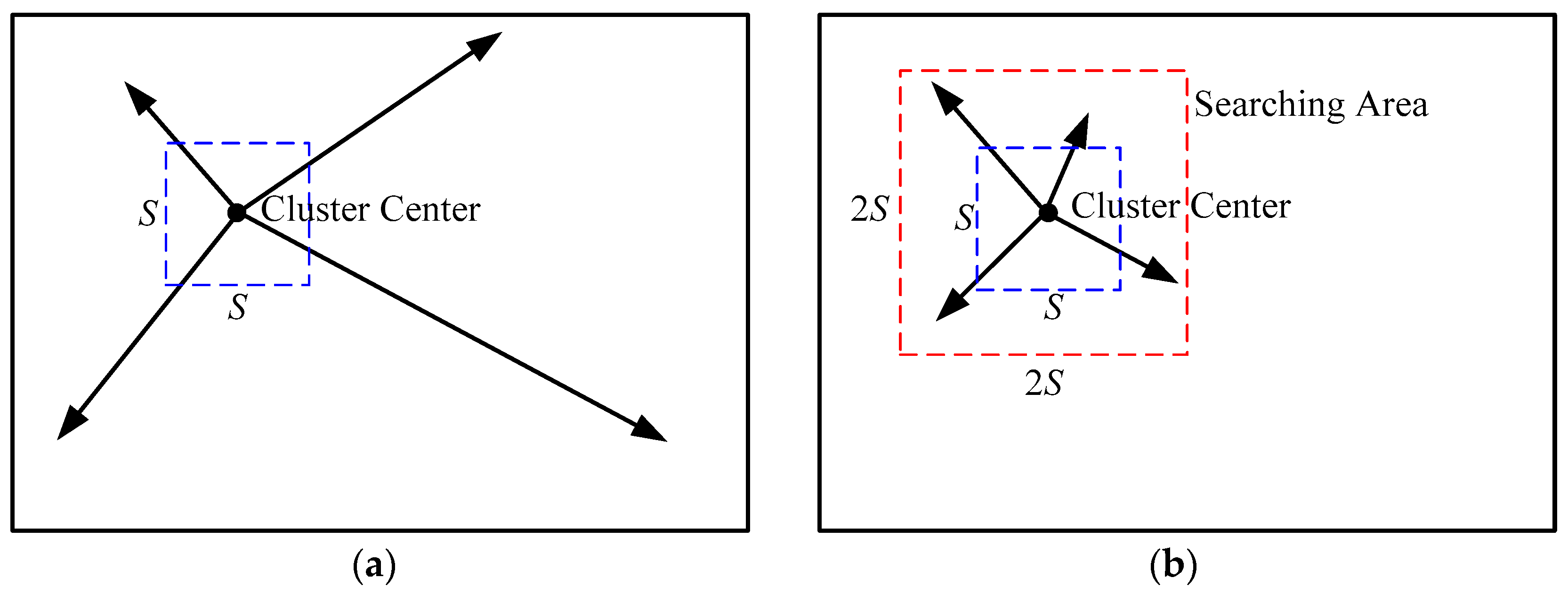
- Initialize cluster centers. Set initial cluster centers on a regular grid spaced pixels apart, and then move these cluster centers to the positions with the lowest gradients in a 3 × 3 neighborhood;
- (2)
- Assign pixels. Designate each pixel to a closest cluster center in a local search space by local KMC;
- (3)
- Update cluster centers. Set each cluster center as the mean of all pixels in the corresponding cluster;
- (4)
- Repeat steps (2)–(3) until the clusters do not change or another given criterion is met;
- (5)
- Post-processing. The CCA is used to reassign isolated regions to nearby superpixels if the size of the isolated regions is smaller than a minimum size .
3. Proposed Likelihood-Based Superpixel Algorithm
3.1. Local Likelihood-Based Clustering
3.2. Local Likelihood-Based Edge Evolving
- (1)
- Estimate the likelihood of pixel intensities within each superpixel and count the total number of edge pixels of all superpixels, denoted by ;
- (2)
- Reassign each edge pixel by Equation (10), and count the total number of edge pixels whose labels have been changed, denoted by ;
- (3)
- Compute the change rate of the edge pixels defined by , indicating the ratio of the number of edge pixels that were modified to the number of total edge pixels;
- (4)
- Repeat steps (1)–(3) until reaches a prespecified small value, i.e., .
3.3. Statistical Modeling of SAR Images by GГD
4. Experiments and Discussion
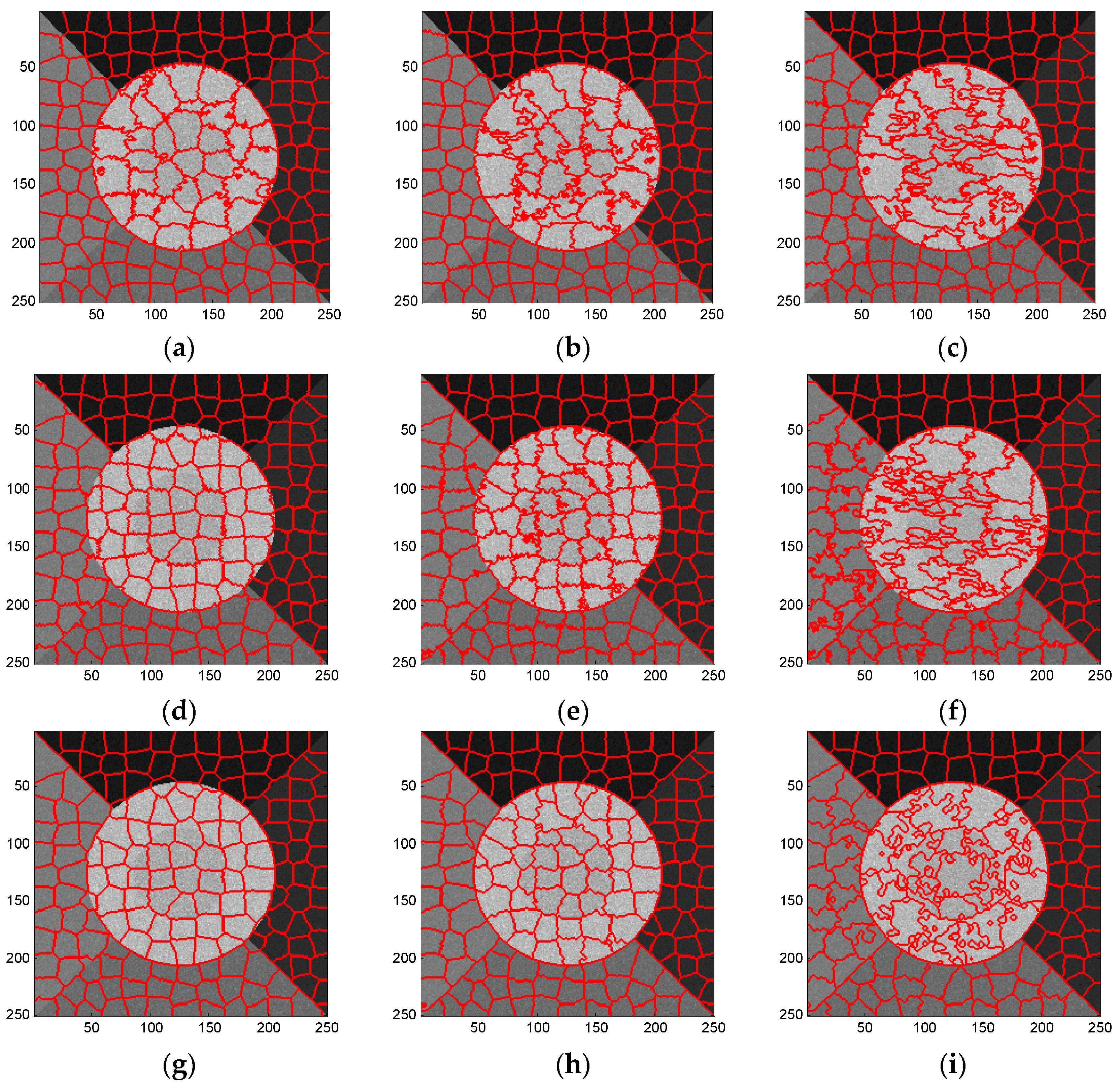
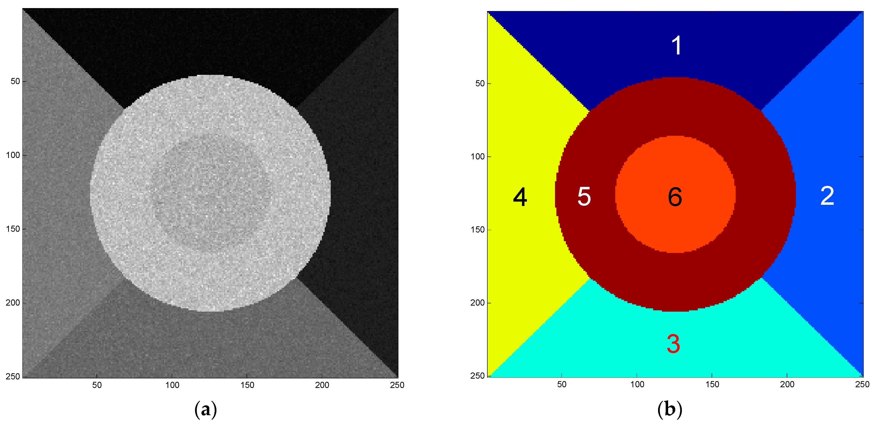
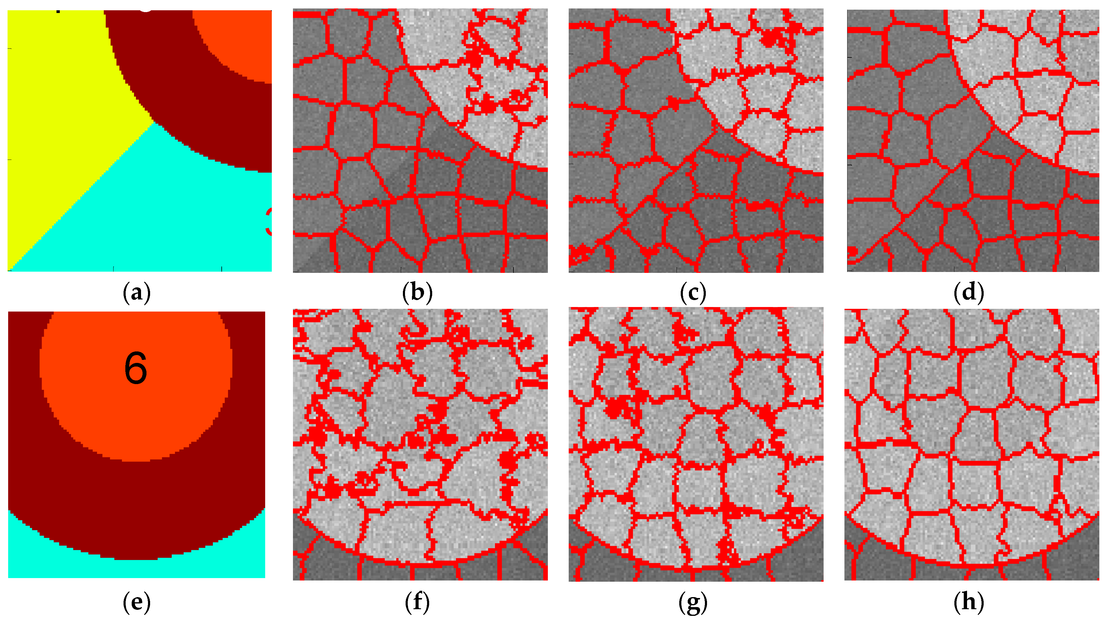
4.1. Evaluation on Simulated SAR Image
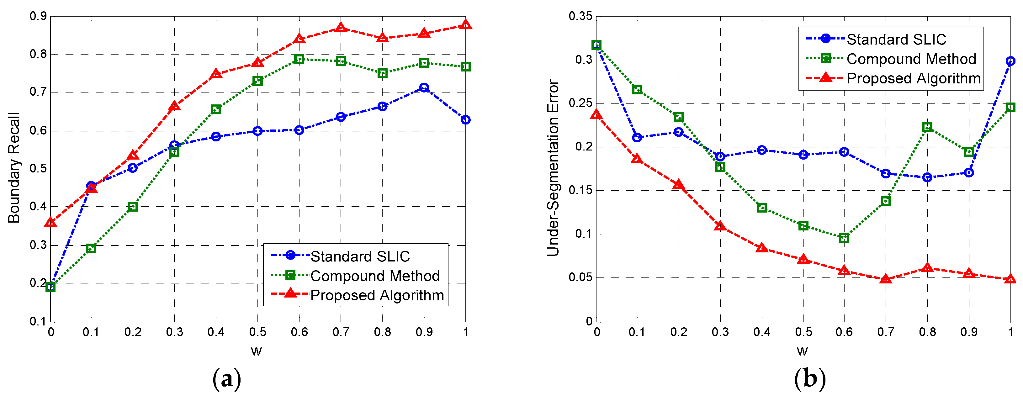
- Boundary recall: The BR computes what fraction of ground truth edges overlap exactly with the boundary pixels of the obtained superpixels, and is computed by:where is the number of boundary pixels shared by the ground truth and the obtained superpixels, and denotes the number of boundary pixels of the ground truth. In our work, the internal boundaries of ground truth and superpixels are used.
- Under-segmentation error: Given ground truth segments and a superpixel output , the under-segmentation error is defined by [10,11]:where, gives the size of the segment in pixels, is the size of the image in pixels, the expression is the intersection or overlapping error of a superpixel with respect to a ground truth segment , and denotes a minimum number of pixels in overlapping .
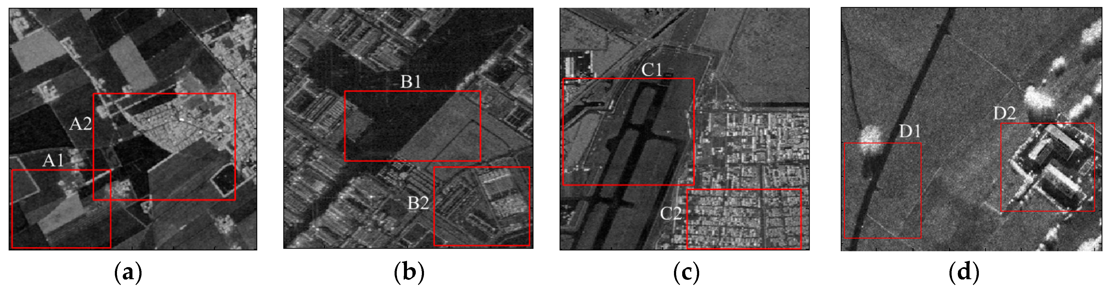
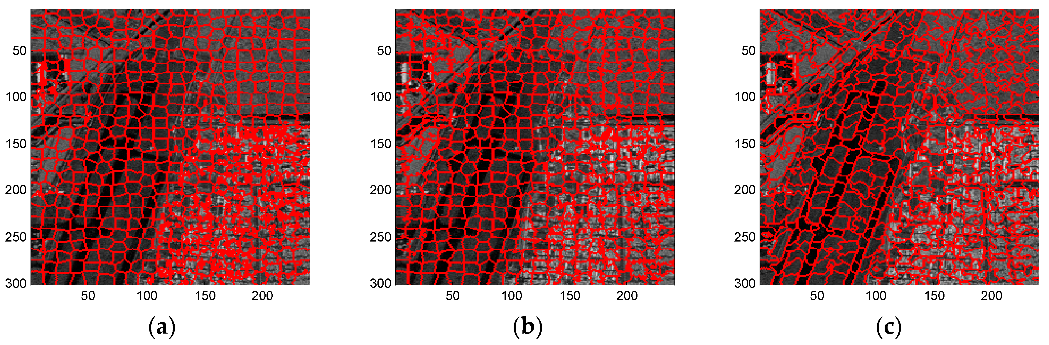
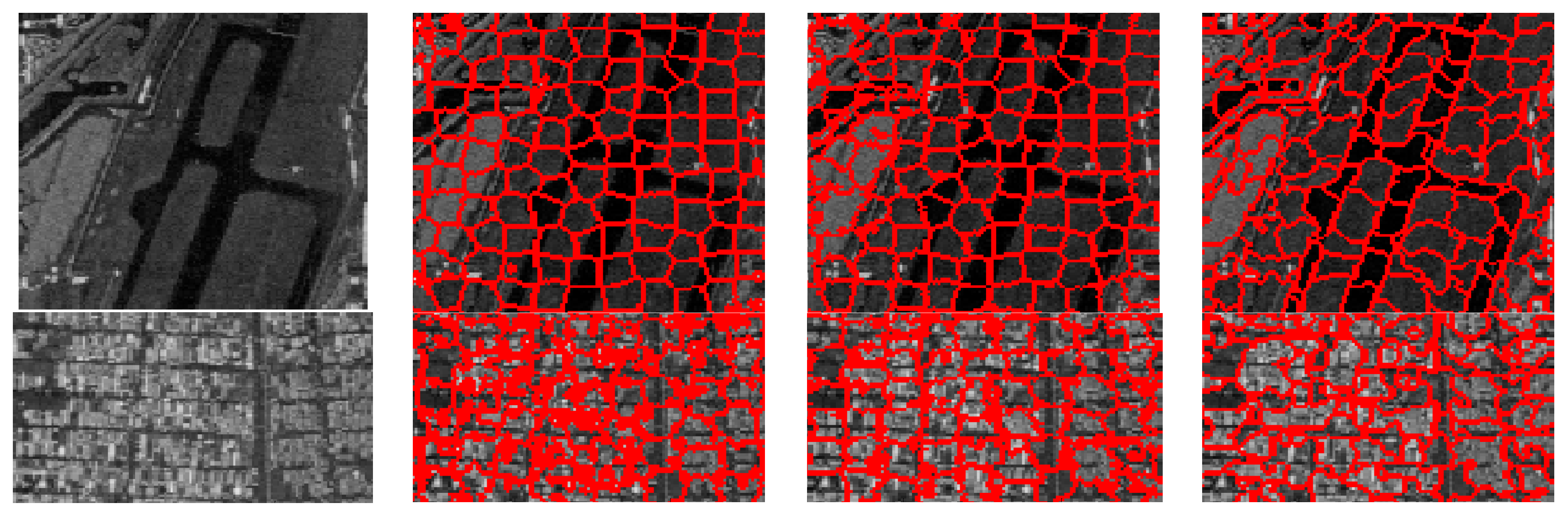
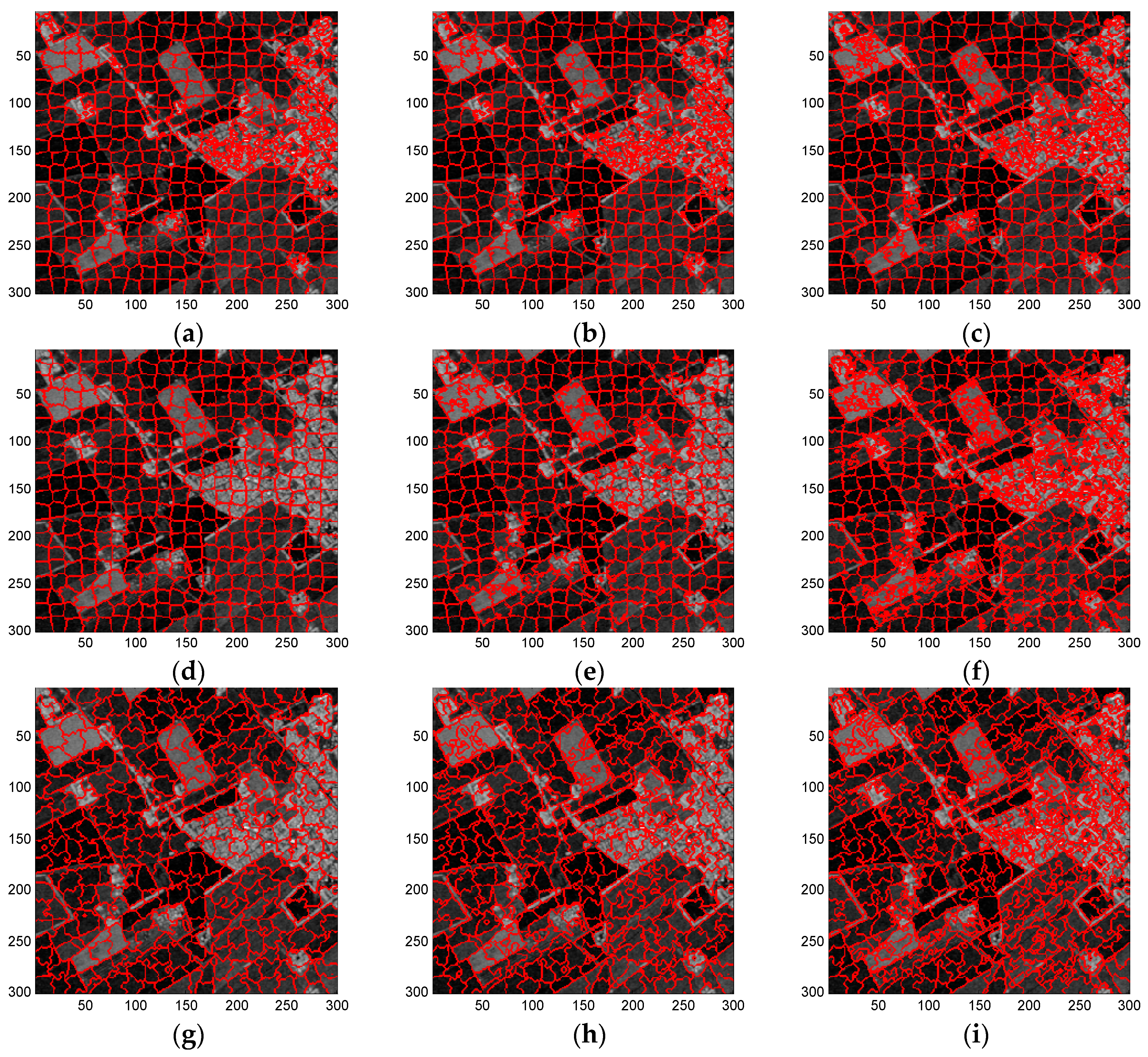
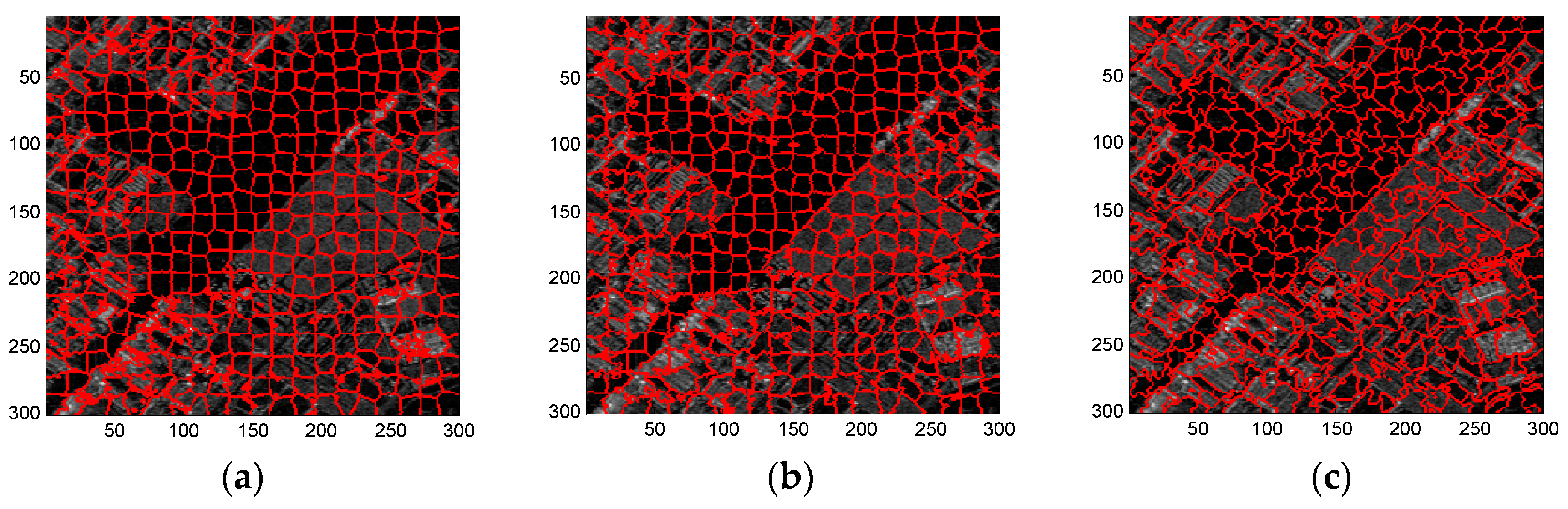
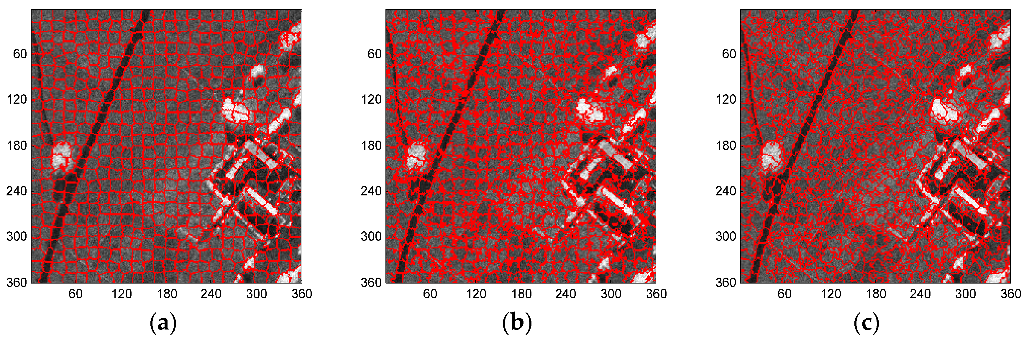
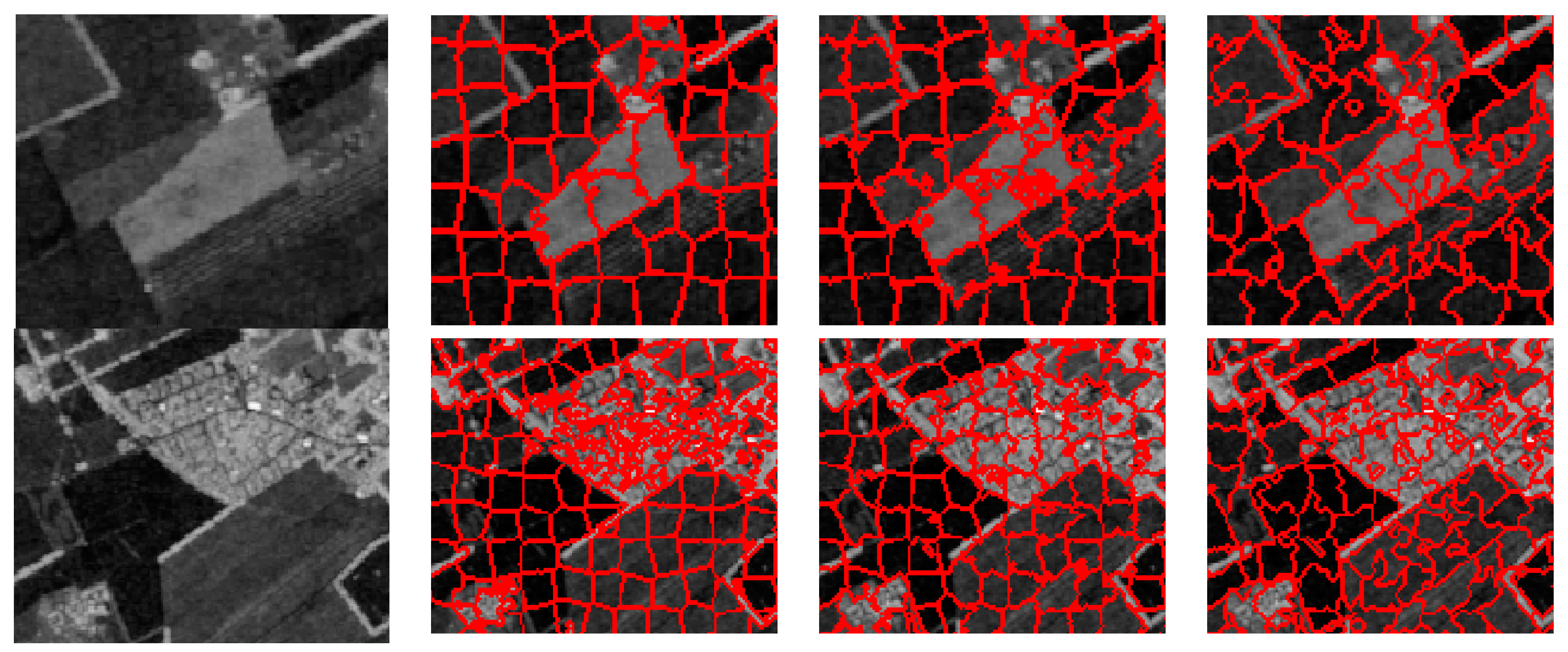
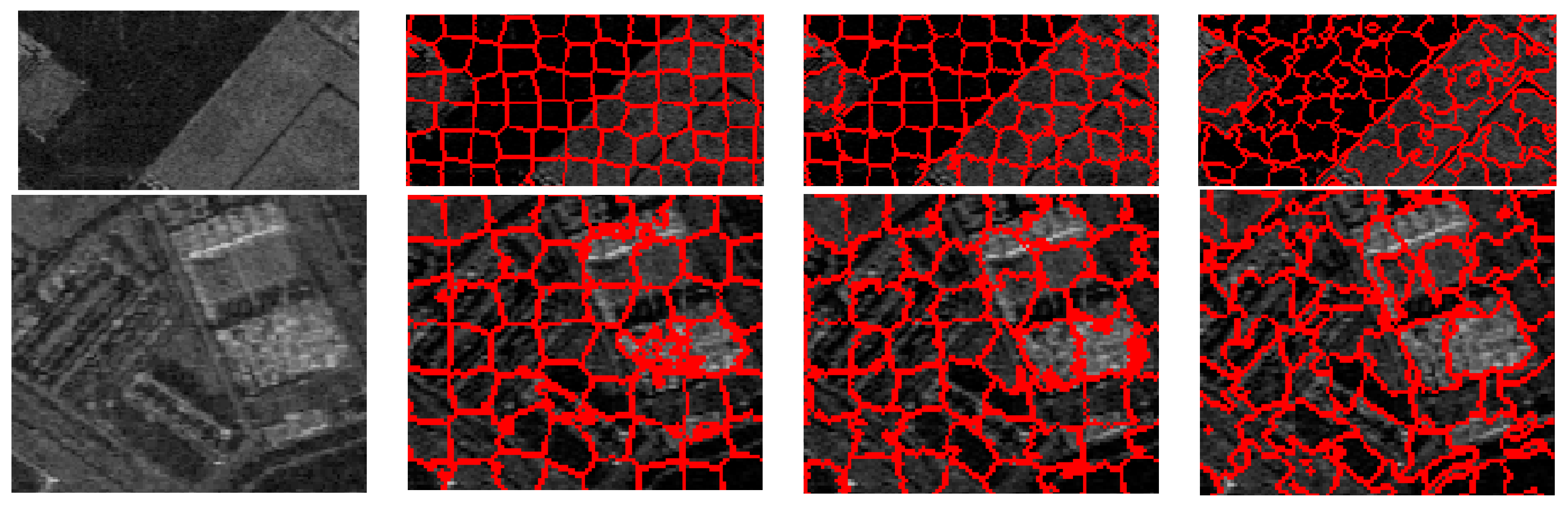
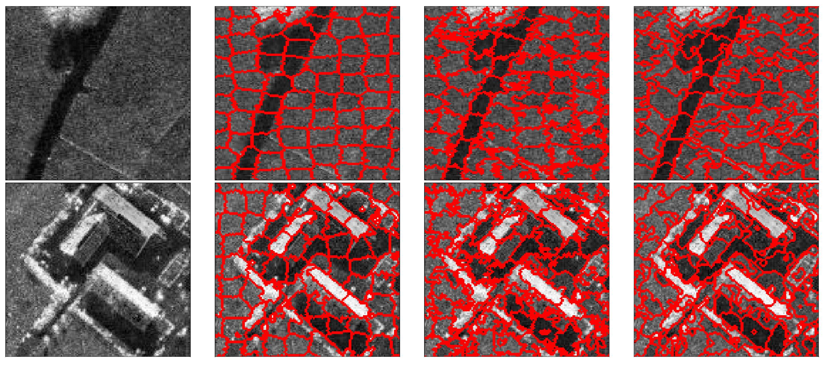
4.2. Evaluation on Real-World SAR Images
5. Conclusions
Acknowledgments
Author Contributions
Conflicts of Interest
References
- Son, N.T.; Chen, C.F.; Chang, N.B.; Chen, C.R. Mangrove mapping and change detection in Ca Mau Peninsula, Vietnam, using Landsat data and object-based image analysis. IEEE J. Sel. Top. Appl. Earth Obs. Remote Sens. 2015, 8, 503–510. [Google Scholar] [CrossRef]
- El Merabet, Y.; Meurie, C.; Ruichek, Y.; Sbihi, A.; Touahni, R. Building roof segmentation from aerial images using a lineand region-based watershed segmentation technique. Sensors 2015, 15, 3172–3203. [Google Scholar] [CrossRef] [PubMed]
- Goodin, D.G.; Anibas, K.L.; Bezymennyi, M. Mapping land cover and land use from object-based classification: An example from a complex agricultural landscape. Int. J. Remote Sens. 2015, 36, 4702–4723. [Google Scholar] [CrossRef]
- Liu, B.; Hu, H.; Wang, H.; Wang, K.; Liu, X.; Yu, W. Superpixel-based classification with an adaptive number of classes for polarimetric SAR images. IEEE Trans. Geosci. Remote Sens. 2013, 51, 907–924. [Google Scholar] [CrossRef]
- Qin, X.; Zou, H.; Zhou, S.; Ji, K. Region-based classification of SAR images using Kullback-Leibler distance between generalized gamma distributions. IEEE Geosci. Remote Sens. Lett. 2015, 12, 1655–1659. [Google Scholar]
- Lu, K.; Li, J.; An, X.; He, H. Vision sensor-based road detection for field robot navigation. Sensors 2015, 15, 29594–29617. [Google Scholar] [CrossRef] [PubMed]
- Sun, X.; Shang, K.; Ming, D.; Tian, J.; Ma, J. A biologically-inspired framework for contour detection using superpixel-based candidates and hierarchical visual cues. Sensors 2015, 15, 26654–26674. [Google Scholar] [CrossRef] [PubMed]
- Wang, C.; Liu, Z.; Chan, S.C. Superpixel-based hand gesture recognition with Kinect depth camera. IEEE Trans. Multimed. 2015, 17, 29–39. [Google Scholar] [CrossRef]
- Shen, J.; Du, Y.; Wang, W.; Li, X. Lazy random walks for superpixel segmentation. IEEE Trans. Image Process. 2014, 23, 1451–1462. [Google Scholar] [CrossRef] [PubMed]
- Achanta, R.; Shaji, A.; Smith, K.; Lucchi, A.; Fua, P.; Süsstrunk, S. SLIC Superpixels; EPFL Technical Report 149300; School of Computer and Communication Sciences, Ecole Polytechnique Fedrale de Lausanne: Lausanne, Switzerland, 2010; pp. 1–15. [Google Scholar]
- Achanta, R.; Shaji, A.; Smith, K.; Lucchi, A.; Fua, P.; Süsstrunk, S. SLIC superpixels compared to state-of-the-art superpixel methods. IEEE Trans. Pattern Anal. Mach. Intell. 2012, 34, 2274–2282. [Google Scholar] [CrossRef] [PubMed]
- Shi, J.; Malik, J. Normalized cuts and image segmentation. IEEE Trans. Pattern Anal. Mach. Intell. 2000, 22, 888–905. [Google Scholar]
- Felzenszwalb, P.F.; Huttenlocher, D.P. Efficient graph-based image segmentation. Int. J. Comput. Vis. 2004, 59, 167–181. [Google Scholar] [CrossRef]
- Vedaldi, A.; Soatto, S. Quick Shift and Kernel Methods for Mode Seeking. In Computer Vision—ECCV 2008; Springer Berlin Heidelberg: Berlin, Germany, 2015; pp. 705–718. [Google Scholar]
- Levinshtein, A.; Stere, A.; Kutulakos, K.N.; Fleet, D.J.; Dickinson, S.J.; Siddiqi, K. Turbopixels: Fast superpixels using geometric flows. IEEE Trans. Pattern Anal. Mach. Intell. 2009, 31, 2290–2297. [Google Scholar] [CrossRef] [PubMed]
- Li, H.C.; Hong, W.; Wu, Y.R.; Fan, P.Z. On the empirical-statistical modeling of SAR images with generalized gamma distribution. IEEE J. Sel. Top. Signal Process. 2011, 5, 386–397. [Google Scholar]
- Duda, R.O.; Hart, P.E.; Stork, D.G. Pattern Classification, 2nd ed.; John Wiley & Sons: Hoboken, NJ, USA, 2012; Volume 4, pp. 30–31. [Google Scholar]
- Qin, X.; Zhou, S.; Zou, H. SAR image segmentation via hierarchical region merging and edge evolving with generalized gamma distribution. IEEE Geosci. Remote Sens. Lett. 2014, 11, 1742–1746. [Google Scholar]
- Li, S.Z. Markov Random Field Modeling in Image Analysis, 3rd ed.; Springer Science & Business Media: New York, NY, USA, 2009; pp. 28–29. [Google Scholar]
- Akbari, V.; Moser, G.; Doulgeris, A.P.; Anfinsen, S.N.; Eltoft, T.; Serpico, B.S. A K-Wishart Markov random field model for clustering of polarimetric SAR imagery. In Proceedings of the IEEE International Geoscience and Remote Sensing Symposium (IGARSS), Vancouver, BC, Canada, 24–29 July 2011; pp. 1357–1360.
- Stacy, E.W. A generalization of the gamma distribution. Ann. Math. Stat. 1962, 33, 1187–1192. [Google Scholar] [CrossRef]
- Nicolas, J.M. Introduction to second kind statistic: Application of log-moments and log-cumulants to SAR image law analysis. Trait. Signal 2002, 19, 139–167. [Google Scholar]
- Moser, G.; Zerubia, J.; Serpico, S.B. SAR amplitude probability density function estimation based on a generalized Gaussian model. IEEE Trans. Image Process. 2006, 15, 1429–1442. [Google Scholar] [CrossRef] [PubMed]
- Qin, X.; Zhou, S.; Zou, H.; Gao, G. Simulation of high-resolution SAR clutter image based on nonlinear transformation method. Syst. Eng. Electron. 2014, 36, 453–357. [Google Scholar]


| Algorithm | Clustering | Post-Processing | Total Time | ||
|---|---|---|---|---|---|
| Scheme | Time | Scheme | Time | ||
| Standard SLIC | KMC | 3.288 | CCA | 0.073 | 3.361 |
| Compound method | LC | 7.957 | CCA | 0.074 | 8.031 |
| Proposed algorithm | LC | 7.957 | EES | 56.754 | 64.711 |
| Figure Number | System | Polarization | Band | Size (Pixels) | Resolution | Acquisition Location | Acquisition Year |
|---|---|---|---|---|---|---|---|
| Figure 7a | EMISAR | HV | L | 300 × 300 | 1.5 m × 0.75 m | Foulum, Denmark | 1998 |
| Figure 7b | AIRSAR | VV | C | 300 × 300 | 13.5 m × 5.5 m | Tokyo, Japan | 2000 |
| Figure 7c | UAVSAR | HH | C | 300 × 240 | 1.67 m × 0.6 m | Gulf Coast, America | 2011 |
| Figure 7d | F-SAR | HH | C | 360 × 360 | 0.6 m × 0.6 m | Kaufbeuren, Germany | 2009 |
| Algorithm | Clustering | Post-Processing | Total Time | ||
|---|---|---|---|---|---|
| Scheme | Time | Scheme | Time | ||
| Standard SLIC | KMC | 12.668 | CCA | 0.112 | 12.780 |
| Compound method | LC | 23.253 | CCA | 0.128 | 23.381 |
| Proposed algorithm | LC | 23.253 | EES | 292.439 | 315.692 |
© 2016 by the authors; licensee MDPI, Basel, Switzerland. This article is an open access article distributed under the terms and conditions of the Creative Commons Attribution (CC-BY) license (http://creativecommons.org/licenses/by/4.0/).
Share and Cite
Zou, H.; Qin, X.; Zhou, S.; Ji, K. A Likelihood-Based SLIC Superpixel Algorithm for SAR Images Using Generalized Gamma Distribution. Sensors 2016, 16, 1107. https://doi.org/10.3390/s16071107
Zou H, Qin X, Zhou S, Ji K. A Likelihood-Based SLIC Superpixel Algorithm for SAR Images Using Generalized Gamma Distribution. Sensors. 2016; 16(7):1107. https://doi.org/10.3390/s16071107
Chicago/Turabian StyleZou, Huanxin, Xianxiang Qin, Shilin Zhou, and Kefeng Ji. 2016. "A Likelihood-Based SLIC Superpixel Algorithm for SAR Images Using Generalized Gamma Distribution" Sensors 16, no. 7: 1107. https://doi.org/10.3390/s16071107