
A Fiber-Coupled Self-Mixing Laser Diode for the Measurement of Young’s Modulus


Abstract
:
1. Introduction
2. Measurement Principle
2.1. Measurement Formula for Young’s Modulus
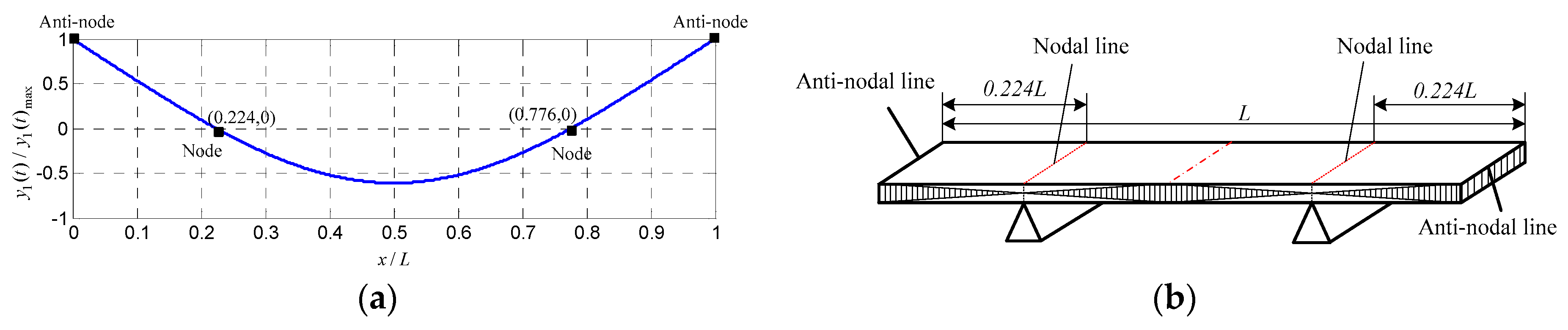
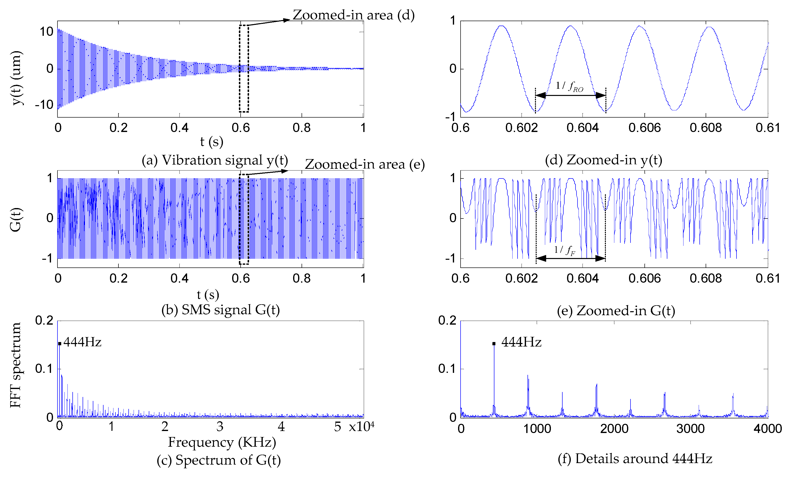
2.2. Vibrating Signals Generated by the Test Specimen
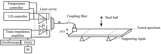
2.3. Capture Using Fiber-Coupled SMLD
3. System Design
3.1. Mechanical Supporting for the Specimen
3.2. Steel Ball for Stimulation
3.3. Requirements for SMLD
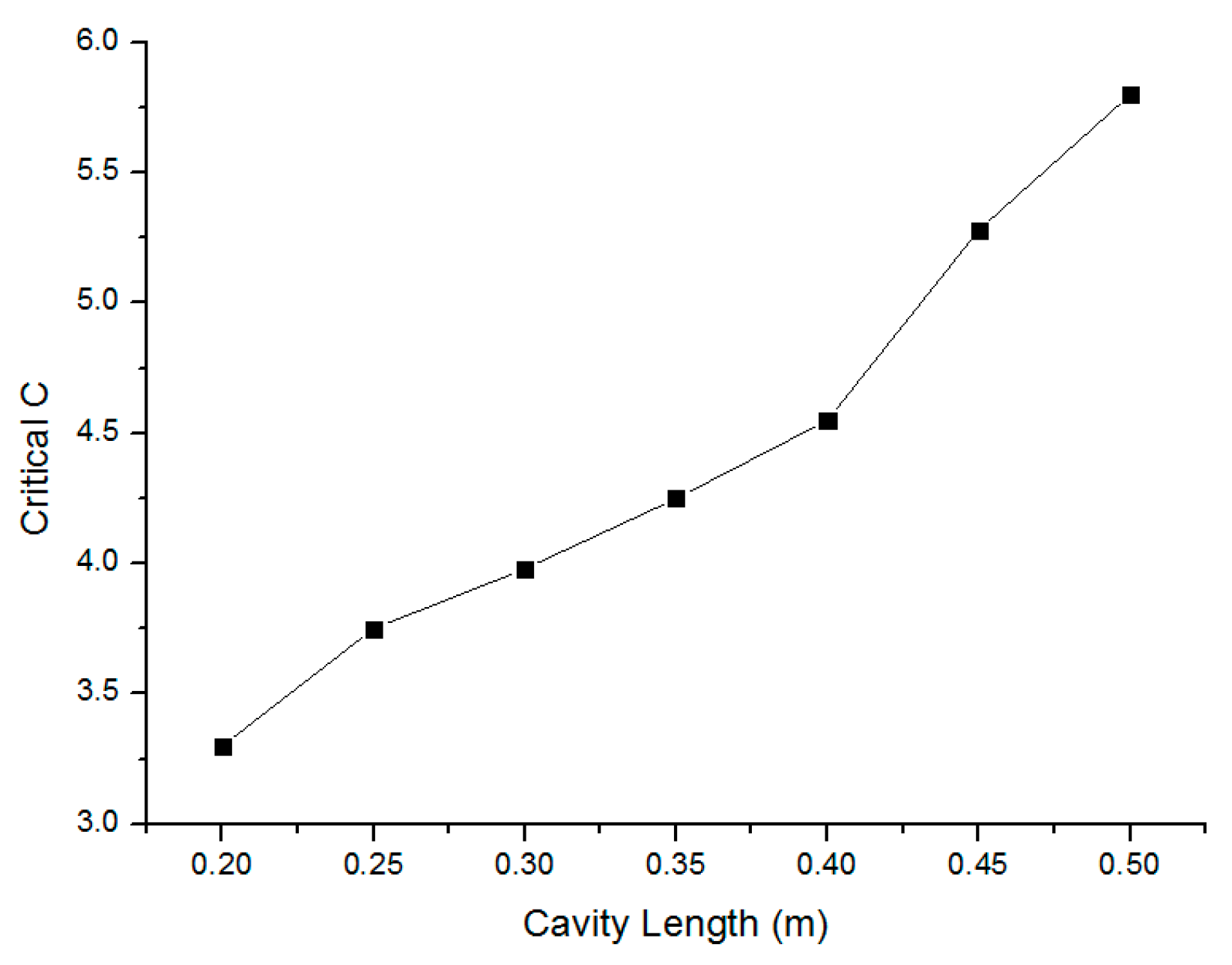
- Step 1: Measure the stability boundary of the SMLD system and from which to determine a suitable external cavity length to place the tested specimen.
- Step 2: Estimate the maximum magnitude by Equation (12). Note that a low , e.g., can be used for the estimation.
- Step 3: Calculate the size of the steel ball using Equations (13) and (15) and .
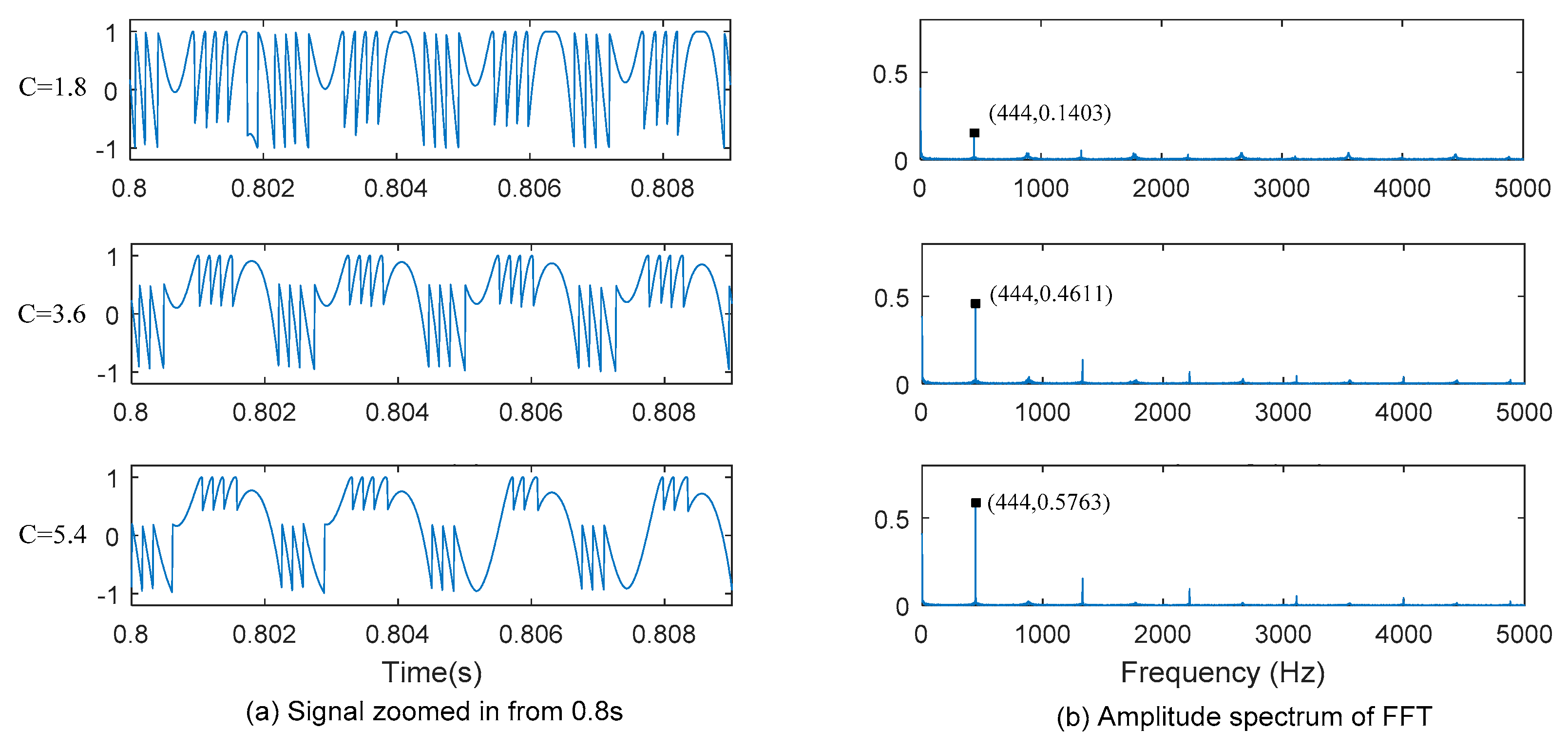
4. Simulations
5. Experiments
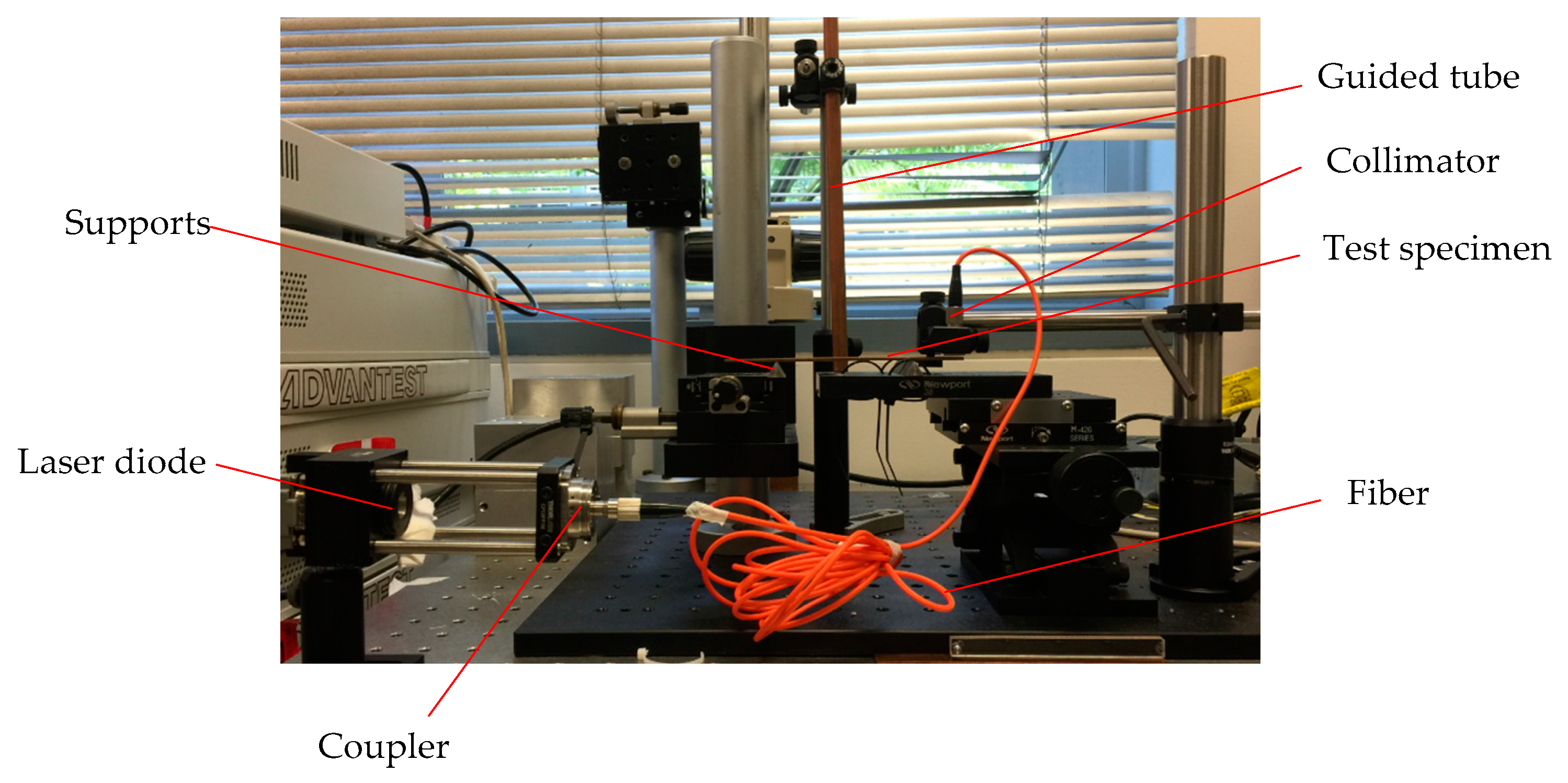
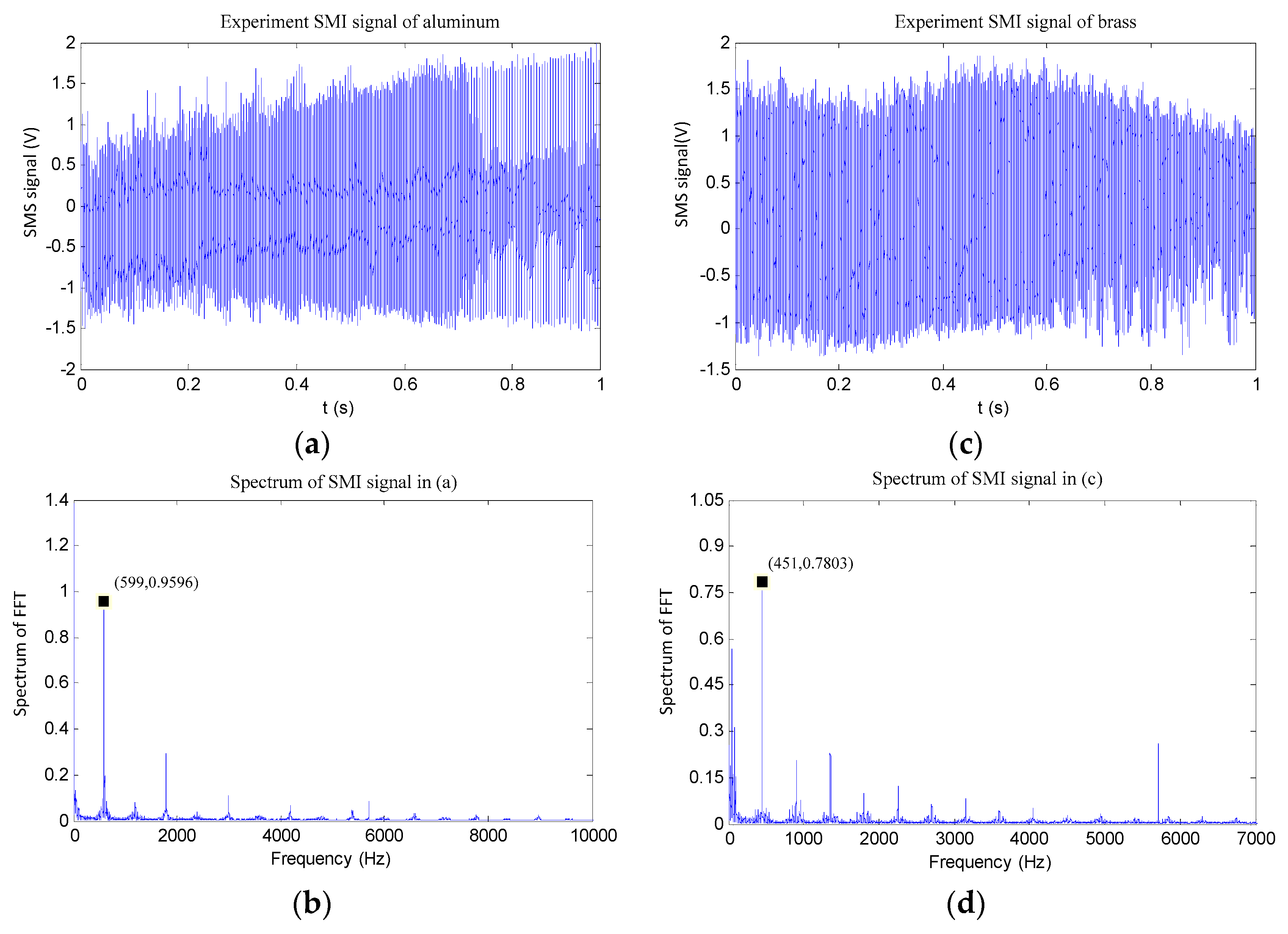
5.1. Experimental Set-up and Results
- Step 1: Install the LD onto a laser mount; set the bias current on the laser controller (LTC100-B from THORLABS) as 52.5 mA and the temperature on the temperature controller (TED200C from THORLABS) is stabilized to 25 ± 0.1 °C.
- Step 2: Install a specimen to be tested and use a coupler (PAF-X-2-B from THORLABS) connected with a step-index multimode fiber optic patch cable (M67L02 from THORLABS) with an adjustable aspheric FC collimators (CFC-2X-B from THORLABS) at the other end to adjust the distance between the specimen and the LD to form an external cavity with 0.5 m long.
- Step 3: Adjust the LD mount so that the fiber-coupled SMLD can be operated in a moderate feedback level by observing the waveform of the SMI signal.
- Step 4: Place the steel ball on the up end of the guided tube and release it. As a result, the specimen is stimulated into vibration. Correspondingly, an SMI signal is produced by the SMLD and recorded by the oscilloscope and the computer through the DAQ card. A LabVIEW script programmed for sampling the SMI signal is set to wait for collecting the signal.
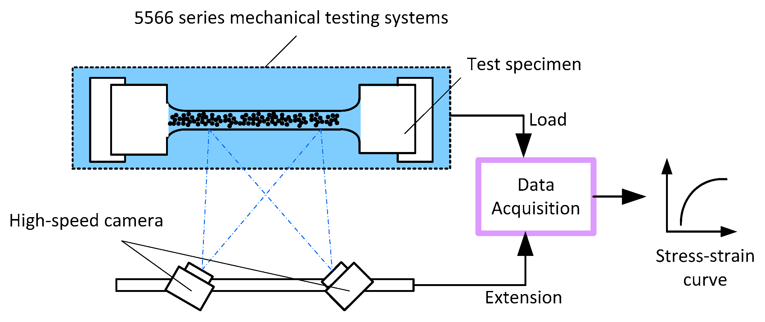
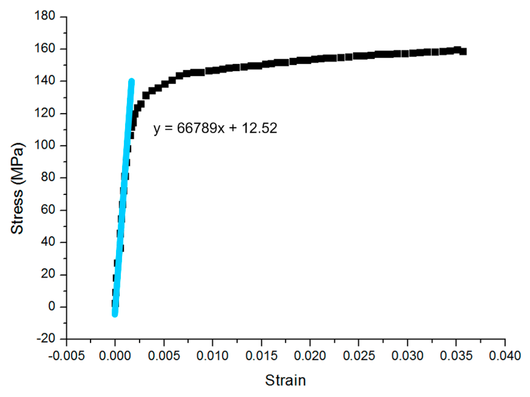
5.2. Comparison with Tensile Testing
6. Conclusions
Acknowledgments
Author Contributions
Conflicts of Interest
Abbreviations
| SMLD | Self-Mixing laser diode |
| LD | Laser Diode |
| PD | Photodiode |
| SMI | Self-mixing interferometry |
| FFT | Fast Fourier Transform |
| DAQ | Data Acquisition |
References
- Lord, J.; Morrell, R. Elastic modulus measurement—Obtaining reliable data from the tensile test. Metrologia 2010, 47, S41. [Google Scholar] [CrossRef]
- Suansuwan, N.; Swain, M.V. Determination of elastic properties of metal alloys and dental porcelains. J. Oral Rehabil. 2001, 28, 133–139. [Google Scholar] [CrossRef] [PubMed]
- Hauptmann, M.; Grattan, K.; Palmer, A.; Fritsch, H.; Lucklum, R.; Hauptmann, P. Silicon resonator sensor systems using self-mixing interferometry. Sens. Actuators A Phys. 1996, 55, 71–77. [Google Scholar] [CrossRef]
- ASTM Standard E 1876-15, Standard Test Method for Dynamic Young’s Modulus, Shear Modulus, and Poisson’s Ratio by Impulse Excitation of Vibration; ASTM International, West Conshohocken, PA, USA. 2005. Available online: www.astm.org/Standards/E1876.htm (accessed on 11 February 2005).
- Ye, X.; Zhou, Z.; Yang, Y.; Zhang, J.; Yao, J. Determination of the mechanical properties of microstructures. Sens. Actuators A Phys. 1996, 54, 750–754. [Google Scholar] [CrossRef]
- Kiesewetter, L.; Zhang, J.-M.; Houdeau, D.; Steckenborn, A. Determination of Young’s moduli of micromechanical thin films using the resonance method. Sens. Actuators A Phys. 1992, 35, 153–159. [Google Scholar] [CrossRef]
- Schmidt, R.; Alpern, P.; Tilgner, R. Measurement of the Young’s modulus of moulding compounds at elevated temperatures with a resonance method. Polym. Test. 2005, 24, 137–143. [Google Scholar] [CrossRef]
- Haines, D.W.; Leban, J.-M.; Herbé, C. Determination of Young’s modulus for spruce, fir and isotropic materials by the resonance flexure method with comparisons to static flexure and other dynamic methods. Wood Sci. Technol. 1996, 30, 253–263. [Google Scholar] [CrossRef]
- Schmidt, R.; Wicher, V.; Tilgner, R. Young’s modulus of moulding compounds measured with a resonance method. Polym. Test. 2005, 24, 197–203. [Google Scholar] [CrossRef]
- Hauert, A.; Rossoll, A.; Mortensen, A. Young’s modulus of ceramic particle reinforced aluminium: Measurement by the Impulse Excitation Technique and confrontation with analytical models. Compos. Part A Appl. Sci. Manuf. 2009, 40, 524–529. [Google Scholar] [CrossRef]
- Yeh, W.-C.; Jeng, Y.-M.; Hsu, H.-C.; Kuo, P.-L.; Li, M.-L.; Yang, P.-M.; Lee, P.H.; Li, P.-C. Young’s modulus measurements of human liver and correlation with pathological findings, in Ultrasonics Symposium. In Proceedings of the 2001 IEEE Ultrasonics Symposium, Atlanta, GA, USA, 7–10 October 2001; pp. 1233–1236.
- Caracciolo, R.; Gasparetto, A.; Giovagnoni, M. Measurement of the isotropic dynamic Young’s modulus in a seismically excited cantilever beam using a laser sensor. J. Sound Vib. 2000, 231, 1339–1353. [Google Scholar] [CrossRef]
- Giuliani, G.; Norgia, M.; Donati, S.; Bosch, T. Laser diode self-mixing technique for sensing applications. J. Opt. 2002, 4, S283–S294. [Google Scholar] [CrossRef]
- Zabit, U.; Bosch, T.; Bony, F. Adaptive transition detection algorithm for a self-mixing displacement sensor. IEEE Sens. J. 2009, 9, 1879–1886. [Google Scholar] [CrossRef]
- Tay, C.; Wang, S.; Quan, C.; Shang, H. Optical measurement of Young’s modulus of a micro-beam. Opt. Laser Technol. 2000, 32, 329–333. [Google Scholar] [CrossRef]
- Comella, B.; Scanlon, M. The determination of the elastic modulus of microcantilever beams using atomic force microscopy. J. Mater. Sci. 2000, 35, 567–572. [Google Scholar] [CrossRef]
- Kang, K.; Kim, K.; Lee, H. Evaluation of elastic modulus of cantilever beam by TA-ESPI. Opt. Laser Technol. 2007, 39, 449–452. [Google Scholar] [CrossRef]
- Yu, Y.; Xi, J.; Chicharo, J.F. Measuring the feedback parameter of a semiconductor laser with external optical feedback. Opt. Express 2011, 19, 9582–9593. [Google Scholar] [CrossRef] [PubMed]
- Wang, M. Fourier transform method for self-mixing interference signal analysis. Opt. Laser Technol. 2001, 33, 409–416. [Google Scholar] [CrossRef]
- Donati, S. Developing self-mixing interferometry for instrumentation and measurements. Laser Photonics Rev. 2012, 6, 393–417. [Google Scholar] [CrossRef]
- Lin, K.; Yu, Y.; Xi, J.; Fan, Y.; Li, H. Measuring Young’s modulus using a self-mixing laser diode. In Proceedings of the S PIE—The International Society for O ptical Engineering, San Francisco, CA, USA, 1 February 2014.
- Lin, K.; Yu, Y.; Xi, J.; Li, H. Design requirements of experiment set-up for self-mixing-based Young’s modulus measurement system. In Proceedings of the TENCON 2015—2015 IEEE Region 10 Conference, Macao, China, 1–4 November 2015; pp. 1–5.
- Schmitz, T.L.; Smith, K.S. Mechanical Vibrations: Modeling and Measurement; Springer Science & Business Media: New York, NY, USA, 2011. [Google Scholar]
- Yu, Y.; Xi, J.; Chicharo, J.F.; Bosch, T. Toward Automatic Measurement of the Linewidth-Enhancement Factor Using Optical Feedback Self-Mixing Interferometry With Weak Optical Feedback. IEEE J. Quantum Electron. 2007, 43, 527–534. [Google Scholar] [CrossRef]
- Yu, Y.; Giuliani, G.; Donati, S. Measurement of the linewidth enhancement factor of semiconductor lasers based on the optical feedback self-mixing effect. IEEE Photonics Technol. Lett. 2004, 16, 990–992. [Google Scholar] [CrossRef]
- Xi, J.; Yu, Y.; Chicharo, J.F.; Bosch, T. Estimating the parameters of semiconductor lasers based on weak optical feedback self-mixing interferometry. IEEE J. Quantum Elect. 2005, 41, 1058–1064. [Google Scholar]
- Fan, Y.; Yu, Y.; Xi, J.; Guo, Q. Dynamic stability analysis for a self-mixing interferometry system. Opt. Express 2014, 22, 29260–29269. [Google Scholar] [CrossRef] [PubMed]
- Yu, Y.; Xi, J.; Chicharo, J.F. Improving the performance in an optical feedback self-mixing interferometry system using digital signal pre-processing. In Proceedings of the IEEE International Symposium on Intelligent Signal Processing, Madrid, Spain, 3–5 October 2007; pp. 1–6.
- Meriam, J.; Kraige, G.; Palm, W. Engineering Mechanics Vol. 1: Statics; John Wiley & Sons: New York, NY, USA, 1987. [Google Scholar]
- Sljapic, V.; Hartley, P.; Pillinger, I. Observations on fracture in axi-symmetric and three-dimensional cold upsetting of brass. J. Mater. Process. Technol. 2002, 125, 267–274. [Google Scholar] [CrossRef]
- Digilov, R.M.; Abramovich, H. Flexural Vibration Test of a Beam Elastically Restrained at One End: A New Approach for Young’ s Modulus Determination. Adv. Mater. Sci. Eng. 2013, 2013, 1–6. [Google Scholar] [CrossRef]
- Czichos, H.; Saito, T.; Smith, L.R. Springer Handbook of Materials Measurement Methods; Springer Science & Business Media: Berlin, Germany, 2006. [Google Scholar]


| Parameters | Physical Meaning | Unit |
|---|---|---|
| Time index. | s | |
| Laser phase with feedback | rad | |
| Feedback level factor | rad | |
| Line-width enhancement factor | - | |
| Interference function which indicates the influence of the optical feedback | - | |
| Interference function which indicates the influence of the optical feedback | - | |
| Modulation index for the laser intensity (typically ) | - | |
| Laser intensity emitted by the free running LD | - | |
| Laser intensity when LD with optical feedback | - |
| Specimen | Aluminum 6061 | Brass | |||
|---|---|---|---|---|---|
| Times (N) | (Hz) | (GPa) | (Hz) | (GPa) | |
| 1 | 599 | 70.2 | 451 | 116.6 | |
| 2 | 598 | 70.0 | 450 | 116.1 | |
| 3 | 599 | 70.2 | 451 | 116.6 | |
| 4 | 598 | 70.0 | 451 | 116.6 | |
| 5 | 597 | 69.7 | 452 | 117.1 | |
| 6 | 598 | 70.0 | 451 | 116.6 | |
| 7 | 599 | 70.2 | 451 | 116.6 | |
| 8 | 598 | 70.0 | 452 | 117.1 | |
| 9 | 599 | 70.2 | 451 | 116.6 | |
| 10 | 598 | 70.0 | 451 | 116.6 | |
| Mean (μ) | 598 | 70.0 | 451 | 116.7 | |
| Standard deviation (σ) | 0.68 | 0.16 | 0.57 | 0.29 | |
| Times (N) | 1 | 2 | 3 | 4 | 5 | 6 | Mean (μ) | Standard Deviation (σ) | Accuracy (σ/ μ%) | |
|---|---|---|---|---|---|---|---|---|---|---|
| Specimen | ||||||||||
| Aluminum 6061 | 60.6 | 64.4 | 76.2 | 67.0 | 73.9 | 63.0 | 67.6 | 6.2 | 9.2 | |
| Brass | 120.3 | 125.6 | 133.4 | 118.6 | 109.6 | 119.4 | 121.1 | 7.9 | 6.5 | |
© 2016 by the authors; licensee MDPI, Basel, Switzerland. This article is an open access article distributed under the terms and conditions of the Creative Commons Attribution (CC-BY) license (http://creativecommons.org/licenses/by/4.0/).
Share and Cite
Lin, K.; Yu, Y.; Xi, J.; Li, H.; Guo, Q.; Tong, J.; Su, L. A Fiber-Coupled Self-Mixing Laser Diode for the Measurement of Young’s Modulus. Sensors 2016, 16, 928. https://doi.org/10.3390/s16060928
Lin K, Yu Y, Xi J, Li H, Guo Q, Tong J, Su L. A Fiber-Coupled Self-Mixing Laser Diode for the Measurement of Young’s Modulus. Sensors. 2016; 16(6):928. https://doi.org/10.3390/s16060928
Chicago/Turabian StyleLin, Ke, Yanguang Yu, Jiangtao Xi, Huijun Li, Qinghua Guo, Jun Tong, and Lihong Su. 2016. "A Fiber-Coupled Self-Mixing Laser Diode for the Measurement of Young’s Modulus" Sensors 16, no. 6: 928. https://doi.org/10.3390/s16060928