
Optimized Sharable-Slot Allocation Using Multiple Channels to Reduce Data-Gathering Delay in Wireless Sensor Networks

Abstract
:
1. Introduction
2. Preliminary
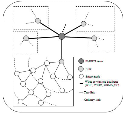
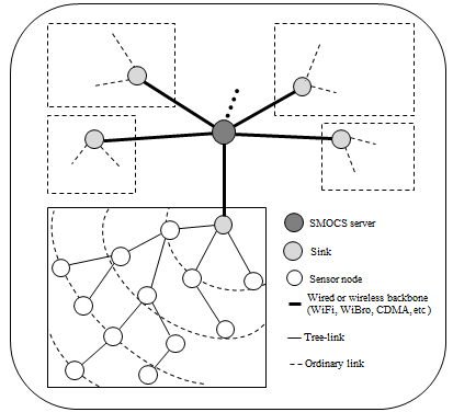
2.1. Network Model
2.2. Notations
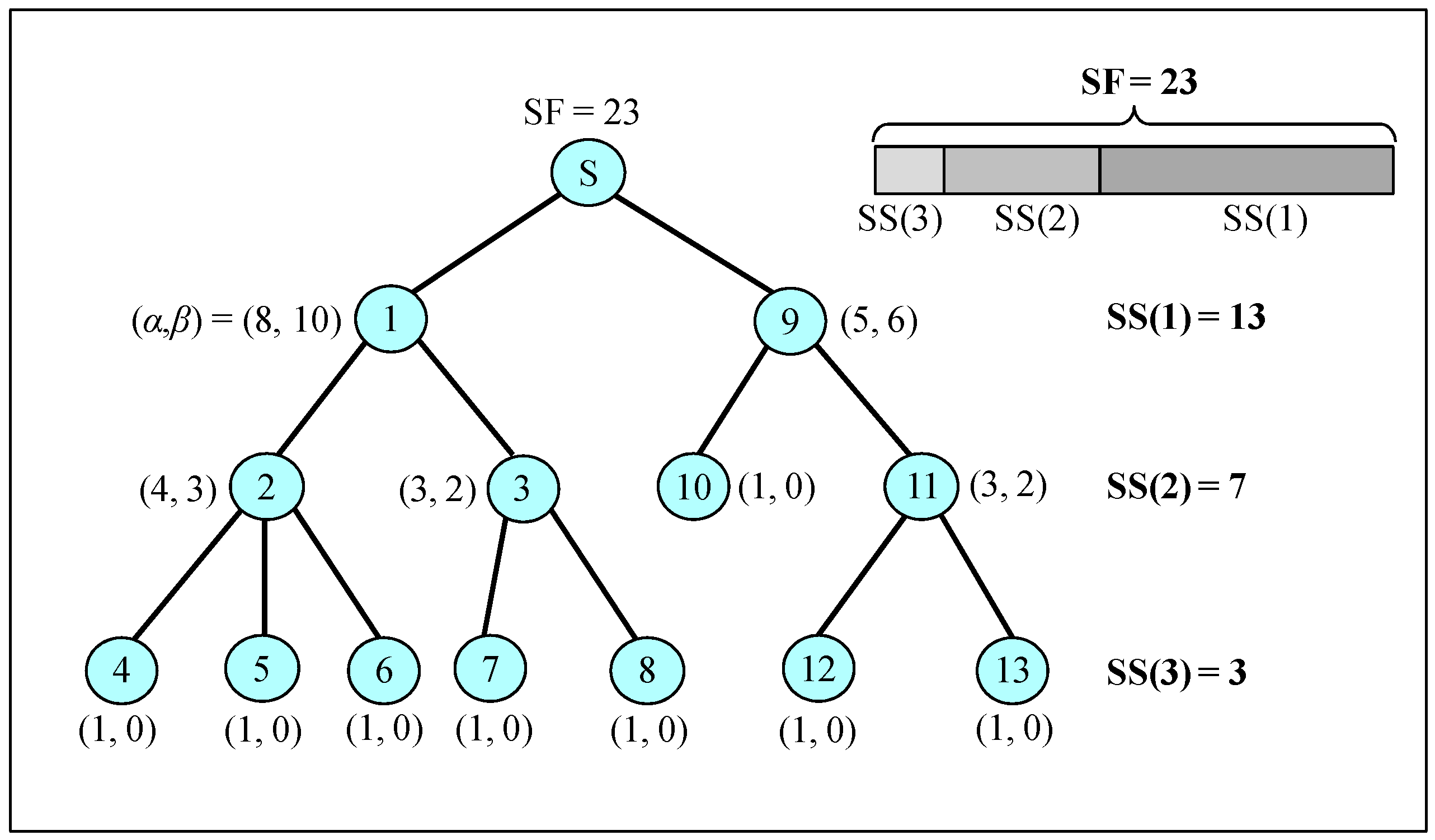
- -
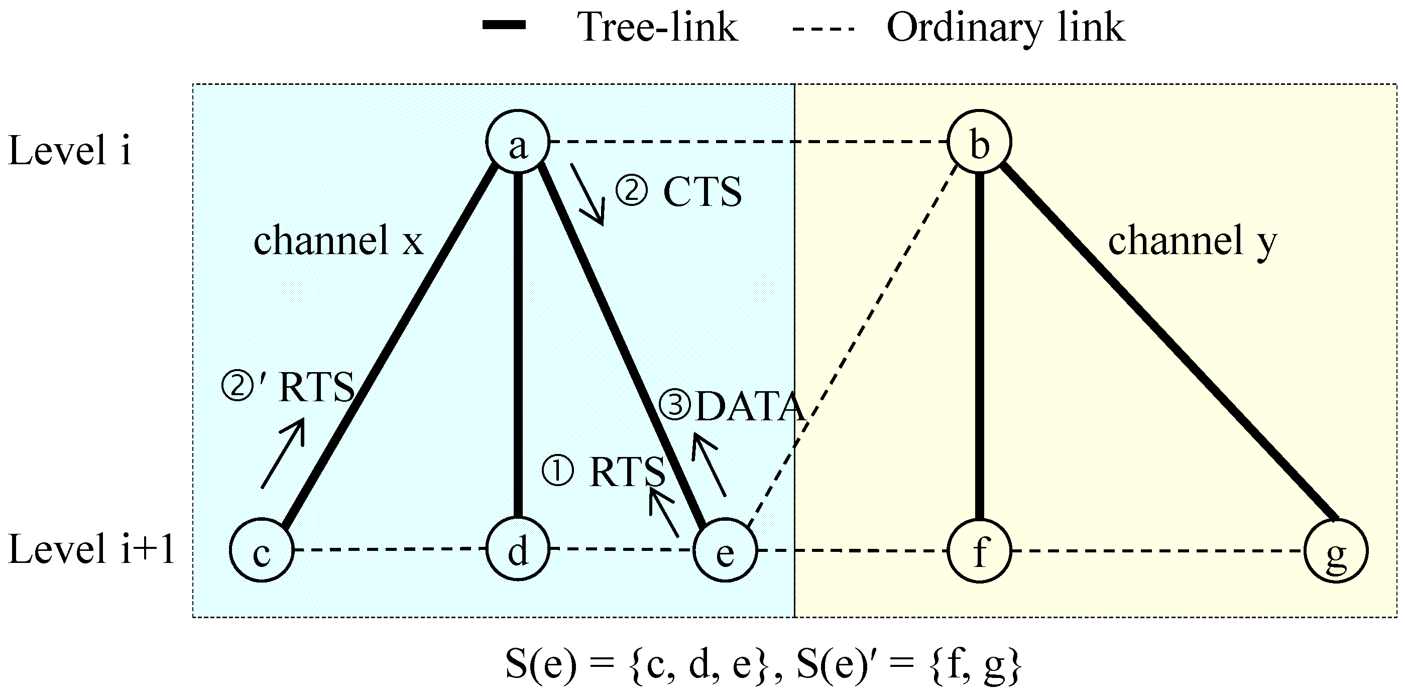
- T(i): A set of nodes that belongs to a tree rooted at node i
- -
- n(l): A set of nodes at level l
- -
- S(i): A sibling group of node i
- -
- S(i)′: n(l) − S(i)
- -
- C(i): Child list for node i
- -
- p(i): Parent of node i
- -
- level(i) or li: Level of node i
- -
- η(i): Number of packets that node i generates during one round of data acquisition
- -
- SS(l): Size of sharable slot for nodes at level l
- -
- SSRx(i) = SSRx(level(i)): Size of sharable slot of node i for receiving data (also indicates receiving sharable slot allocated to the level to which node i belongs)
- -
- SSTx(i) = SSTx(level(i)): Size of sharable slot of node i for sending data (also indicates sending sharable slot allocated to the level to which node i belongs)
- -
- H: Highest level of a given tree
2.3. Problem Identification
3. Protocol Design
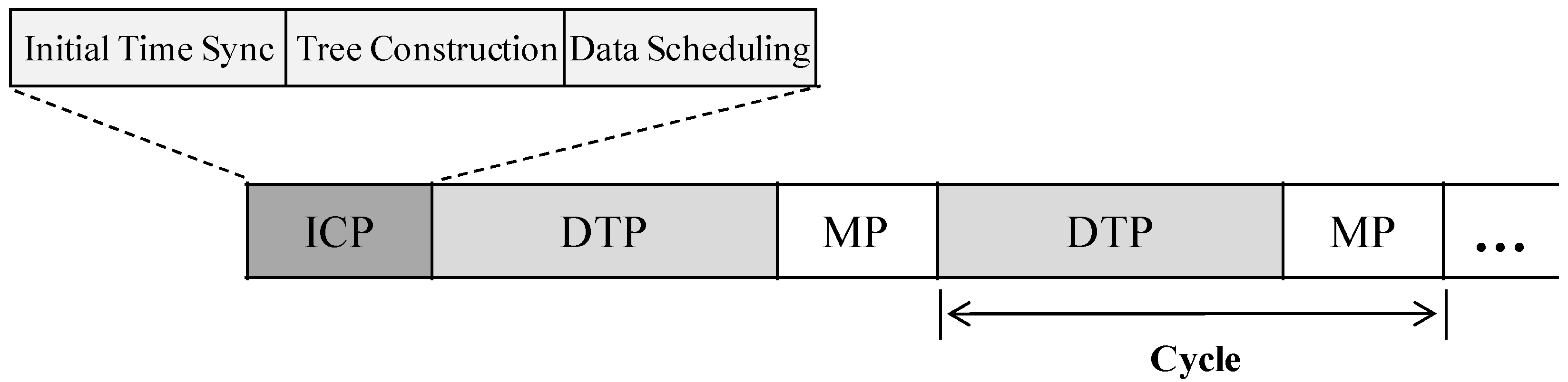
3.1. Time Frame Structure
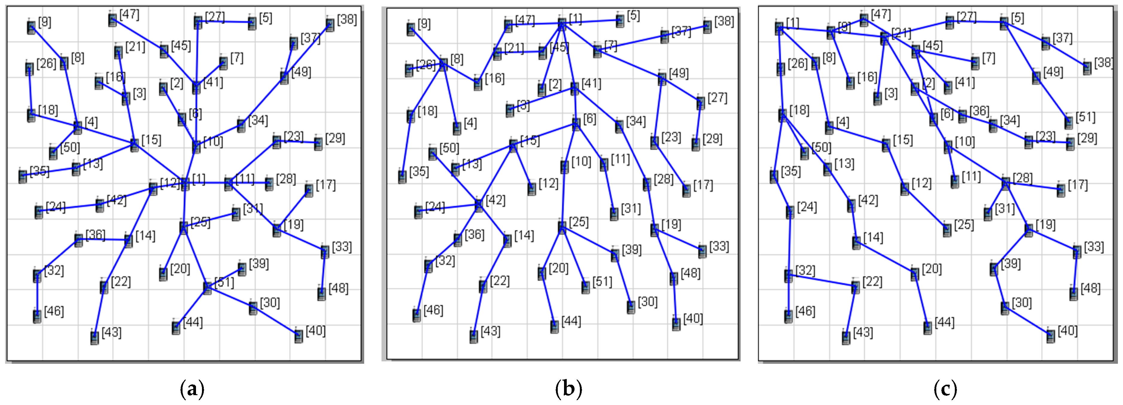
3.2. Tree Construction
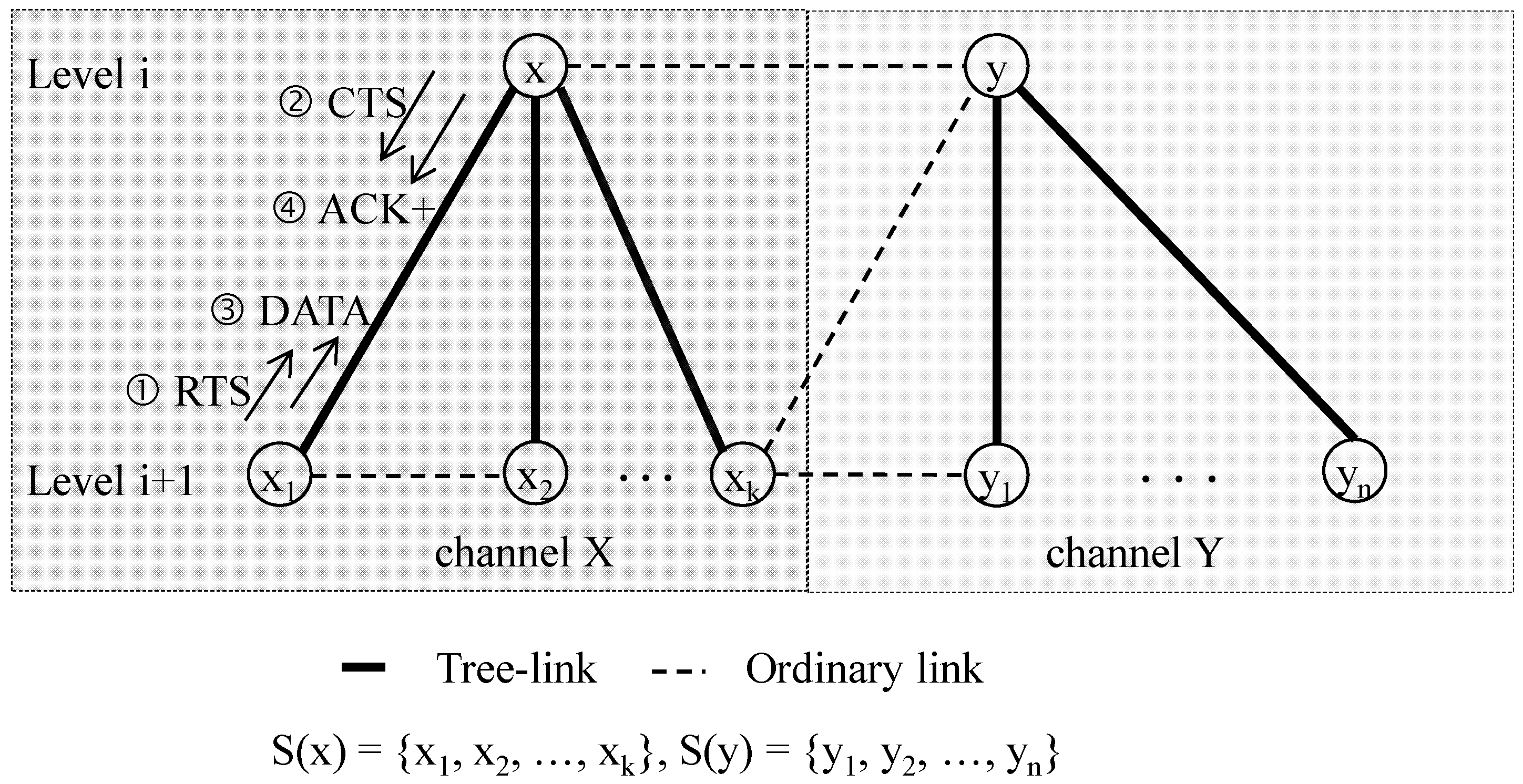
3.3. Channel and Slot Scheduling
3.3.1. Distributed Channel Allocation
3.3.2. Bandwidth Demand Calculation
3.3.3. Sharable Slot Size
3.3.4. Slot Scheduling
3.4. Data Transmission and Recovery
3.4.1. Data Transmission
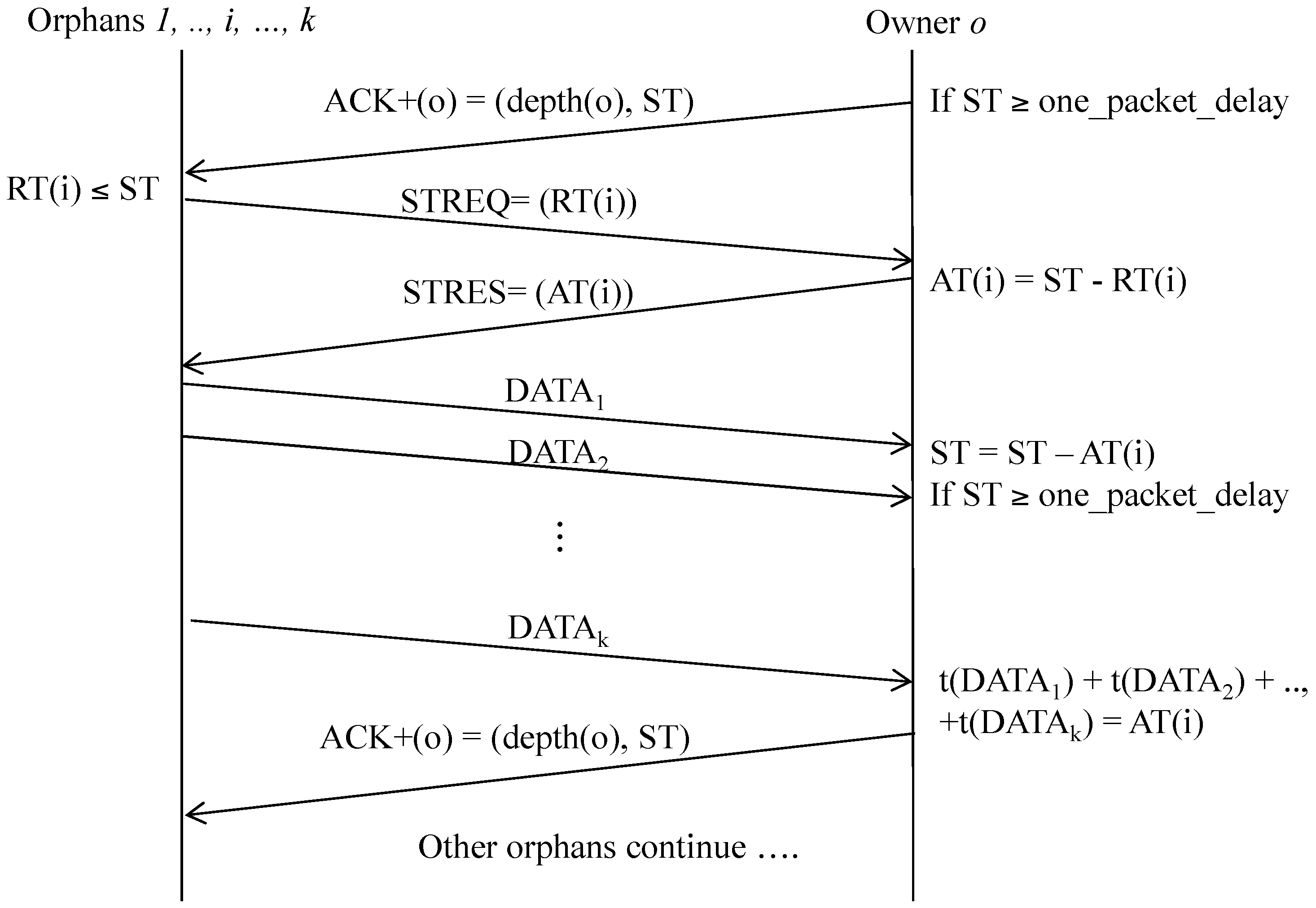
3.4.2. Spare Time Utilization
(a) Spare time announcement
(b) Spare time utilization
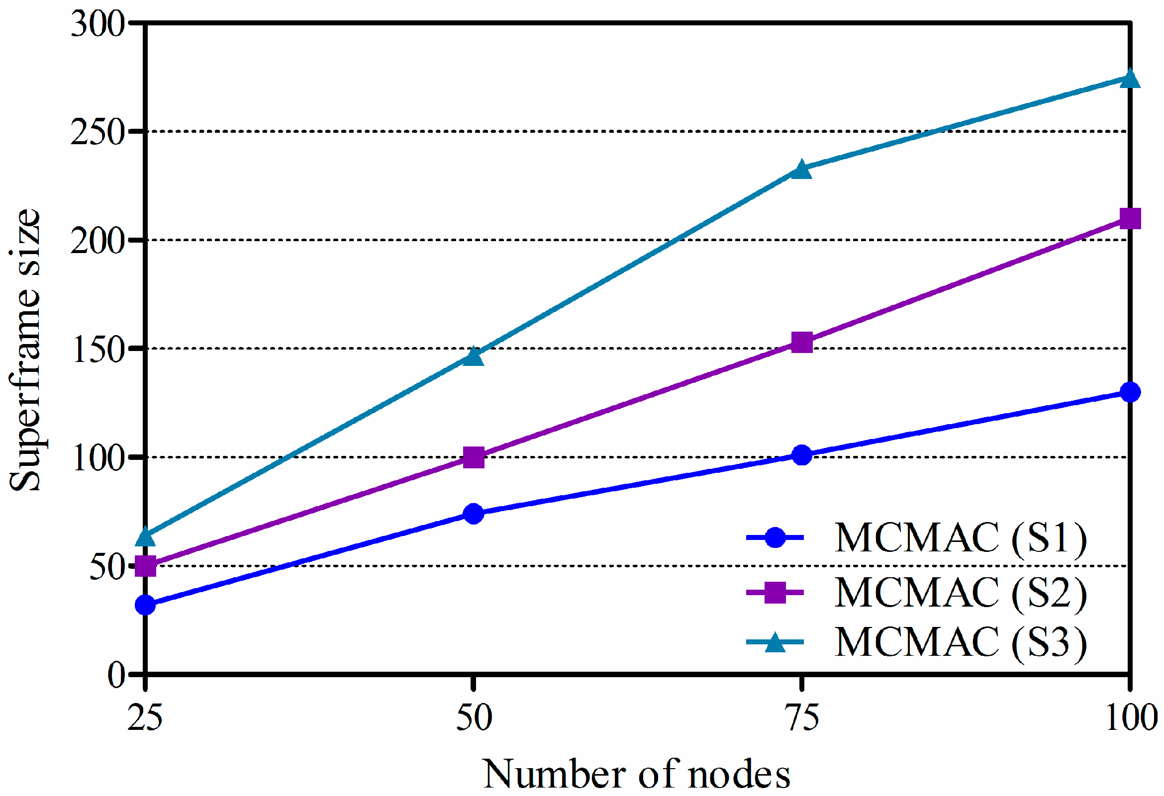
3.5. One Packet Delay and Superframe Size
4. Performance Evaluation
4.1. Simulation Setup
4.2. Simulation Results and Discussions
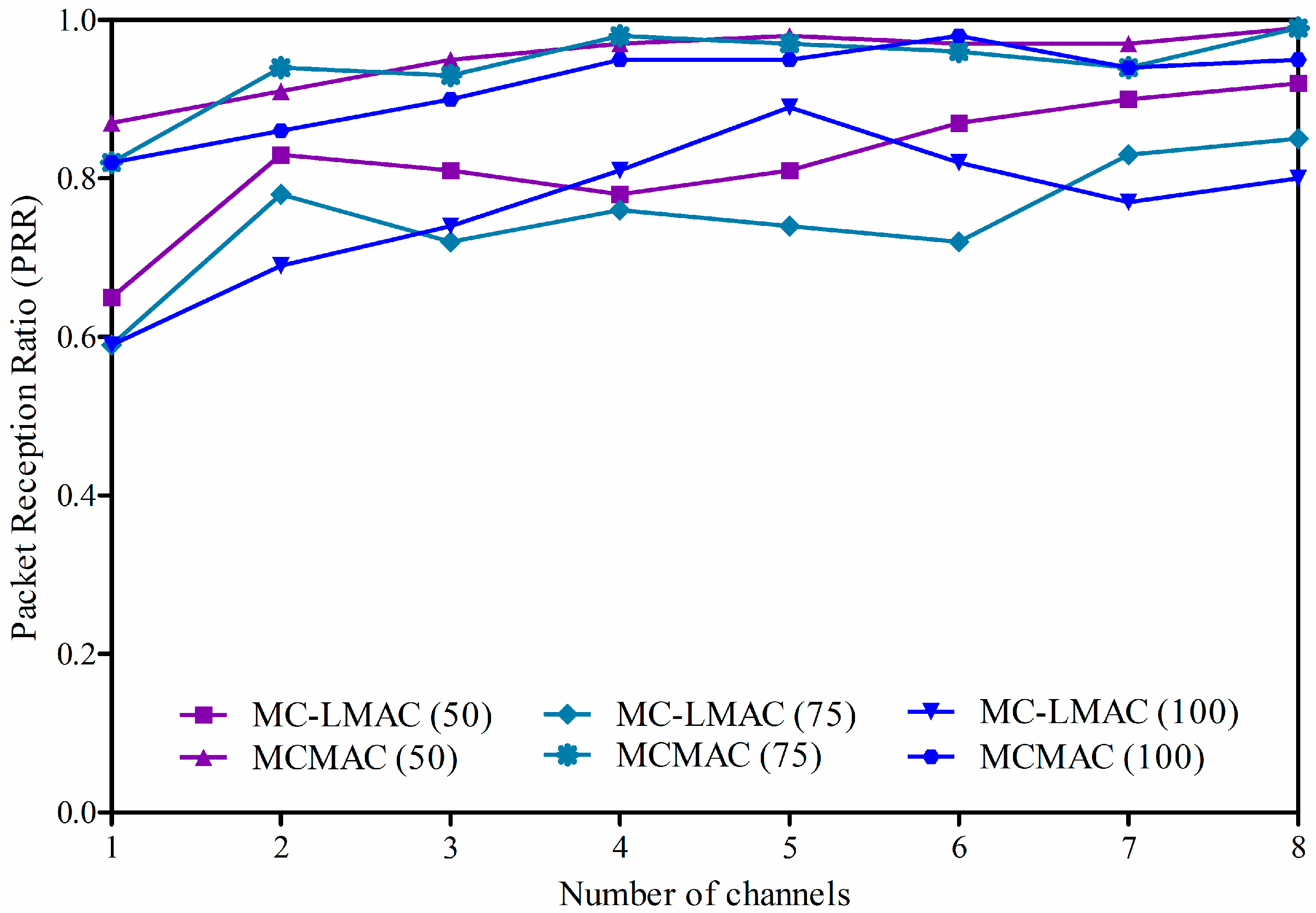
4.2.1. Packet Reception Ratio
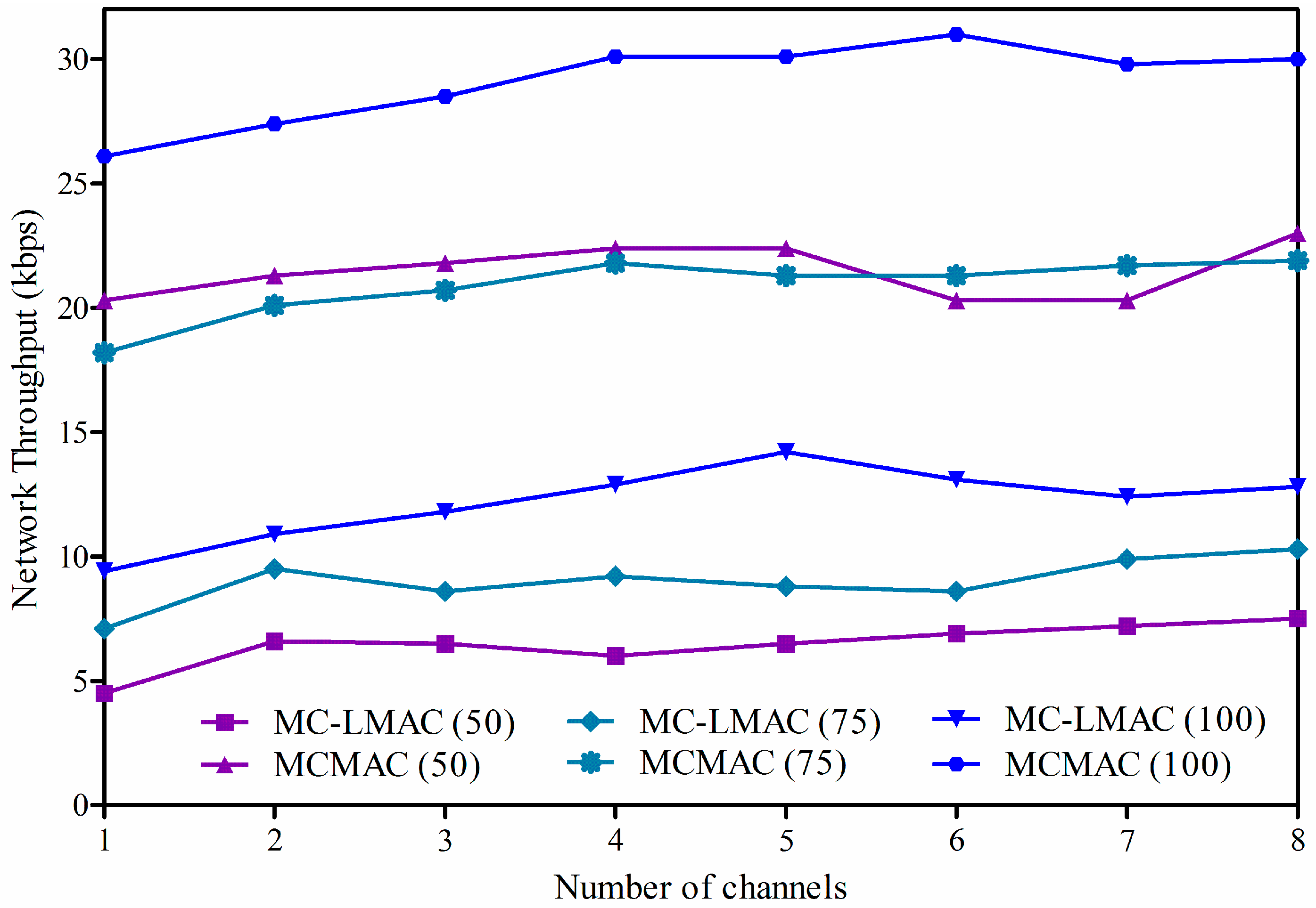
4.2.2. Network Throughput
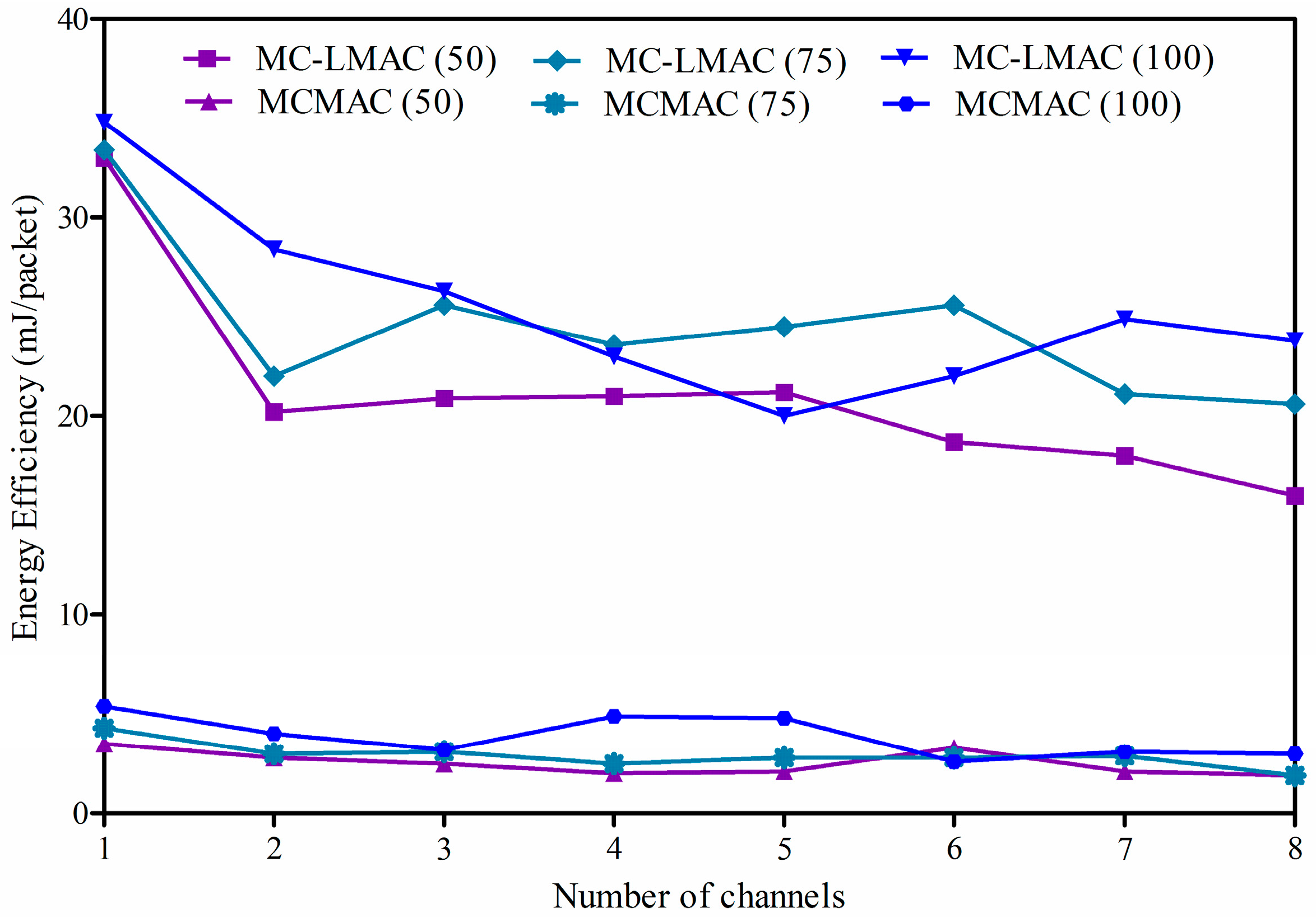
4.2.3. Energy Efficiency
5. Conclusions and Future Works
Acknowledgments
Author Contributions
Conflicts of Interest
References
- Oh, H.; Van Vinh, P. Design and implementation of a MAC protocol for timely and reliable delivery of command and data in dynamic wireless sensor networks. Sensors 2013, 13, 13228–13257. [Google Scholar] [CrossRef] [PubMed]
- Ye, W.; Heidemann, J.; Estrin, D. Medium access control with coordinated adaptive sleeping for wireless sensor networks. IEEE/ACM Trans. Netw. 2004, 12, 493–506. [Google Scholar] [CrossRef]
- Dam, T.V.; Langendoen, K. An adaptive energy-efficient MAC protocol for wireless sensor networks. In Proceedings of the 1st International Conference on Embedded Networked Sensor Systems, Los Angeles, CA, USA, 5–7 November 2003; ACM: New York, NY, USA, 2003; pp. 171–180. [Google Scholar]
- Polastre, J.; Hill, J.; Culler, D. Versatile low power media access for wireless sensor networks. In Proceedings of the 2nd International Conference on Embedded Networked Sensor Systems, Baltimore, MD, USA, 3–5 November 2004; ACM: New York, NY, USA, 2004; pp. 95–107. [Google Scholar]
- Sha, L.; Kai-Wei, F.; Sinha, P. CMAC: An Energy Efficient MAC Layer Protocol Using Convergent Packet Forwarding for Wireless Sensor Networks. In Proceedings of the 4th Annual IEEE Communications Society Conference on Sensor, Mesh and Ad Hoc Communications and Networks (SECON ’07), San Diego, CA, USA, 18–21 June 2007; pp. 11–20.
- Suriyachai, P.; Brown, J.; Roedig, U. Time-critical data delivery in wireless sensor networks. In Proceedings of the 6th IEEE International Conference on Distributed Computing in Sensor Systems, Santa Barbara, CA, USA, 21–23 June 2010; Springer-Verlag: Berlin, Germany, 2010; pp. 216–229. [Google Scholar]
- Le, C.; Baihai, Z.; Lingguo, C.; Qiao, L.; Zhuang, M. Tree-based delay guaranteed and energy efficient MAC protocol for wireless sensor networks. In Proceedings of the Industrial Control and Electronics Engineering (ICICEE) Conference, Xi’an, China, 23–25 August 2012; pp. 893–897.
- Arifuzzaman, M.; Matsumoto, M.; Sato, T. An intelligent hybrid MAC with traffic-differentiation-based QoS for wireless sensor networks. IEEE Sens. 2013, 13, 2391–2399. [Google Scholar] [CrossRef]
- Singh, B.K.; Tepe, K.E. Feedback Based Real-Time MAC (RT-MAC) Protocol for Wireless Sensor Networks. In Proceedings of the IEEE Global Telecommunications Conference (GLOBECOM 2009), Honolulu, HI, USA, 30 November–4 December 2009; pp. 1–6.
- Song, W.Z.; Huang, R.; Shirazi, B.; LaHusen, R. TreeMAC: Localized TDMA MAC Protocol for Real-Time High-Data-Rate Sensor Networks. In Proceedings of IEEE International Conference on Pervasive Computing and Communications (PerCom 2009), Galveston, TX, USA, 9–13 March 2009; pp. 1–10.
- Zhou, G.; Huang, C.; Yan, T.; He, T.; Stankovic, J.A.; Abdelzaher, T.F. MMSN: Multi-frequency media access control for wireless sensor networks. In Proceedings of the 25th IEEE International Conference on Computer Communications, Barcelona, Spain, 23–29 April 2006; pp. 1–13.
- Incel, O.D.; van Hoesel, L.; Jansen, P.; Havinga, P. MC-LMAC: A multi-channel MAC protocol for wireless sensor networks. Ad Hoc Netw. 2011, 9, 73–94. [Google Scholar] [CrossRef]
- Kim, Y.; Shin, H.; Cha, H. Y-MAC: An energy-efficient multi-channel MAC protocol for dense wireless sensor networks. In Proceedings of the 7th international conference on Information processing in sensor networks, St. Louis, MO, USA, 22–24 April 2008; pp. 53–63.
- Jovanovic, M.D.; Djordjevic, G.L. TFMAC: Multi-channel MAC protocol for wireless sensor networks. In Proceedings of the 8th Telecommunications in Modern Satellite, Cable and Broadcasting Services Conference, Serbia, 26–28 September 2007; pp. 23–26.
- Yafeng, W.; Stankovic, J.A.; Tian, H.; Shan, L. Realistic and efficient multi-channel communications in wireless sensor networks. In Proceedings of the 27th Conference on Computer Communications, Phoenix, AZ, USA, 13–18 April 2008.
- Tang, L.; Sun, Y.; Gurewitz, O.; Johnson, D.B. EM-MAC: A dynamic multichannel energy-efficient MAC protocol for wireless sensor networks. In Proceedings of the 12th ACM International Symposium on Mobile Ad Hoc Networking and Computing, Paris, France, 16–20 May 2011; pp. 1–11.
- Van Vinh, P.; Oh, H. O-MAC: An optimized MAC protocol for concurrent data transmission in real-time wireless sensor networks. Wirel. Netw. 2015, 21, 1847–1861. [Google Scholar] [CrossRef]
- Petersen, S.; Carlsen, S. Wirelesshart versus ISA100.11a: The format war hits the factory floor. IEEE Ind. Electron. Mag. 2011, 5, 23–34. [Google Scholar] [CrossRef]
- Saifullah, A.; Xu, Y.; Lu, C.; Chen, Y. Real-time scheduling for wirelesshart networks. In Proceedings of the 31st IEEE Real-Time Systems Symposium (RTSS) Conference, 30 November–3 December 2010; pp. 150–159.
- Han, S.; Zhu, X.; Mok, A.K.; Chen, D.; Nixon, M. Reliable and real-time communication in industrial wireless mesh networks. In Proceedings of the 17th IEEE Real-Time and Embedded Technology and Applications Symposium (RTAS) Conference, Chicago, IL, USA, 11–14 April 2011; pp. 3–12.
- Dezfouli, B.; Radi, M.; Whitehouse, K.; Abd Razak, S.; Hwee-Pink, T. DICSA: Distributed and concurrent link scheduling algorithm for data gathering in wireless sensor networks. Ad Hoc Netw. 2015, 25, 54–71. [Google Scholar] [CrossRef]
- Dezfouli, B.; Radi, M.; Chipara, O. Real-time communication in low-power mobile wireless networks. In Proceedings of the 13th Annual IEEE Consumer Communications & Networking Conference (CCNC), Las Vegas, NV, USA, 9–12 January 2016.
- HART Communication Protocol and Foundation. Available online: http//www.hartcomm2.org (acessed on 6 April 2016).
- Palattella, M.R.; Accettura, N.; Dohler, M.; Grieco, L.A.; Boggia, G. Traffic aware scheduling algorithm for reliable low-power multi-hop IEEE 802.15.4e networks. In Proceedings of the 23rd IEEE International Symposium on Personal Indoor and Mobile Radio Communications (PIMRC), Sydney, Australia, 9–12 September 2012; pp. 327–332.
- Accettura, N.; Palattella, M.R.; Boggia, G.; Grieco, L.A.; Dohler, M. Decentralized traffic aware scheduling for multi-hop low power lossy networks in the internet of things. In Proceedings of the 14th IEEE International Symposium and Workshops on a World of Wireless, Mobile and Multimedia Networks (WoWMoM), Madrid, Spain, 4–7 June 2013; pp. 1–6.
- Soua, R.; Minet, P.; Livolant, E. Wave: A Distributed Scheduling Algorithm for Convergecast in IEEE 802.15.4e TSCH Networks. Trans. Emerging Telecommun. Technol. 2015. [Google Scholar] [CrossRef]
- Yu, B.; Li, J.; Li, Y. Distributed Data Aggregation Scheduling in Wireless Sensor Networks. In Proceedings of the 28th Conference on Computer Communications (INFOCOM 2009), Rio De Janeiro, Brazil, 19–25 April 2009; pp. 2159–2167.
- Chen, X.; Hu, X.; Zhu, J. Minimum data aggregation time problem in wireless sensor networks. LNCS 2005, 3794, 133–142. [Google Scholar]
- Malhotra, B.; Nikolaidis, I.; Nascimento, M.A. Aggregation convergecast scheduling in wireless sensor networks. Wirel. Netw. 2011, 17, 319–335. [Google Scholar] [CrossRef]
- Bagaa, M.; Younis, M.; Ksentini, A.; Badache, N. Reliable multi-channel scheduling for timely dissemination of aggregated data in wireless sensor networks. J. Netw. Comput. Appl. 2014, 46, 293–304. [Google Scholar] [CrossRef]
- Bagaa, M.; Younis, M.; Djenouri, D.; Derhab, A.; Badache, N. Distributed low-latency data aggregation scheduling in wireless sensor networks. ACM Trans. Sen. Netw. 2015, 11, 1–36. [Google Scholar] [CrossRef]
- Bagaa, M.; Challal, Y.; Ksentini, A.; Derhab, A.; Badache, N. Data aggregation scheduling algorithms in wireless sensor networks: Solutions and challenges. IEEE Commun. Surveys Tutor. 2014, 16, 1339–1368. [Google Scholar] [CrossRef]
- Oh, H.; Azad, M.A.K. A big slot scheduling algorithm for the reliable delivery of real-time data packets in wireless sensor networks. In Proceedings of the Wireless Communications, Networking and Applications Conference, Shenzhen, China, 27–28 December 2014; pp. 13–25.
- Borms, J.; Steenhaut, K.; Lemmens, B. Low-overhead dynamic multi-channel MAC for wireless sensor networks. In Proceedings of the European Conference on Wireless Sensor Networks, Coimbra, Portugal, 17–19 February 2010; pp. 81–96.
- Elson, J.; Girod, L.; Estrin, D. Fine-Grained Network Time Synchronization Using Reference Broadcasts. In Proceedings of the 5th Symposium Operating System Design and Implementation, Boston, MA, USA, 9–11 December 2002; pp. 2860–2864.
- Maroti, M.; Kusy, B.; Simon, G.; Ledeczi, A. The Flooding Time Synchronization Protocol. In Proceedings of the 2nd International Conference on Embedded Networked Sensor Systems 2004, Baltimore, MD, USA, 3–5 November 2004; pp. 39–49.
- Greunen, J.V.; Rabaey, J.; Chen, Y.S.; Sheu, J.P. Lightweight Time Synchronization for Wireless Networks. In Proceedings of the 2nd ACM International Conference on Wireless Sensor Networks and Applications, San Diego, CA, USA, 19 September 2003; pp. 11–19.
- QualNet Simulator. Available online: http://web.scalable-networks.com/content/qualnet (acessed on 6 April 2016).
- CC2420 Datasheet, TI. Available online: http://www.ti.com/product/CC2420 (accessed on 6 April 2016).


| Parameter | Value |
|---|---|
| Number of nodes (nNodes) | 50−100 |
| Payload length | 32 bytes |
| Noise factor | 10 dB |
| Path loss model | Two-ray |
| Shadowing model | Constant |
| Fading model | Rician |
| Sensor energy model | MicaZ |
| Transmission power | −25 dBm |
| Dimensions | 100 × 100 m2 |
| Simulation time | 600 s |
| Number of frequencies | 1–8 |
| MAC protocols | MC-LMAC, MCMAC |
| Routing protocol | Tree-based routing |
| Node placement | Random |
© 2016 by the authors; licensee MDPI, Basel, Switzerland. This article is an open access article distributed under the terms and conditions of the Creative Commons by Attribution (CC-BY) license (http://creativecommons.org/licenses/by/4.0/).
Share and Cite
Van Vinh, P.; Oh, H. Optimized Sharable-Slot Allocation Using Multiple Channels to Reduce Data-Gathering Delay in Wireless Sensor Networks. Sensors 2016, 16, 505. https://doi.org/10.3390/s16040505
Van Vinh P, Oh H. Optimized Sharable-Slot Allocation Using Multiple Channels to Reduce Data-Gathering Delay in Wireless Sensor Networks. Sensors. 2016; 16(4):505. https://doi.org/10.3390/s16040505
Chicago/Turabian StyleVan Vinh, Phan, and Hoon Oh. 2016. "Optimized Sharable-Slot Allocation Using Multiple Channels to Reduce Data-Gathering Delay in Wireless Sensor Networks" Sensors 16, no. 4: 505. https://doi.org/10.3390/s16040505