
High-Order Interference Effect Introduced by Polarization Mode Coupling in Polarization—Maintaining Fiber and Its Identification

Abstract
:1. Introduction
2. Model and Analysis
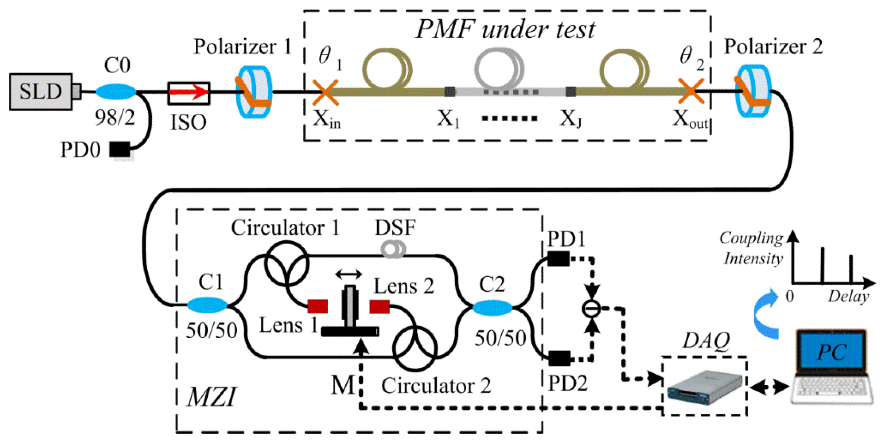
2.1. WLI System with a Large Dynamic Range
2.2. Optical Path Tracking (OPT) Method
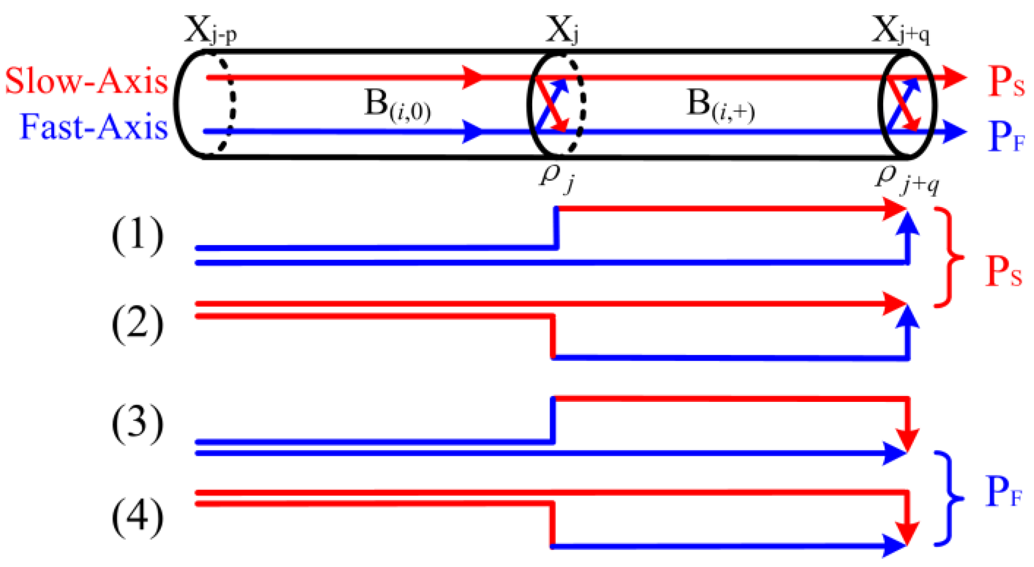
2.2.1. Stable Unit and Recursion Formula
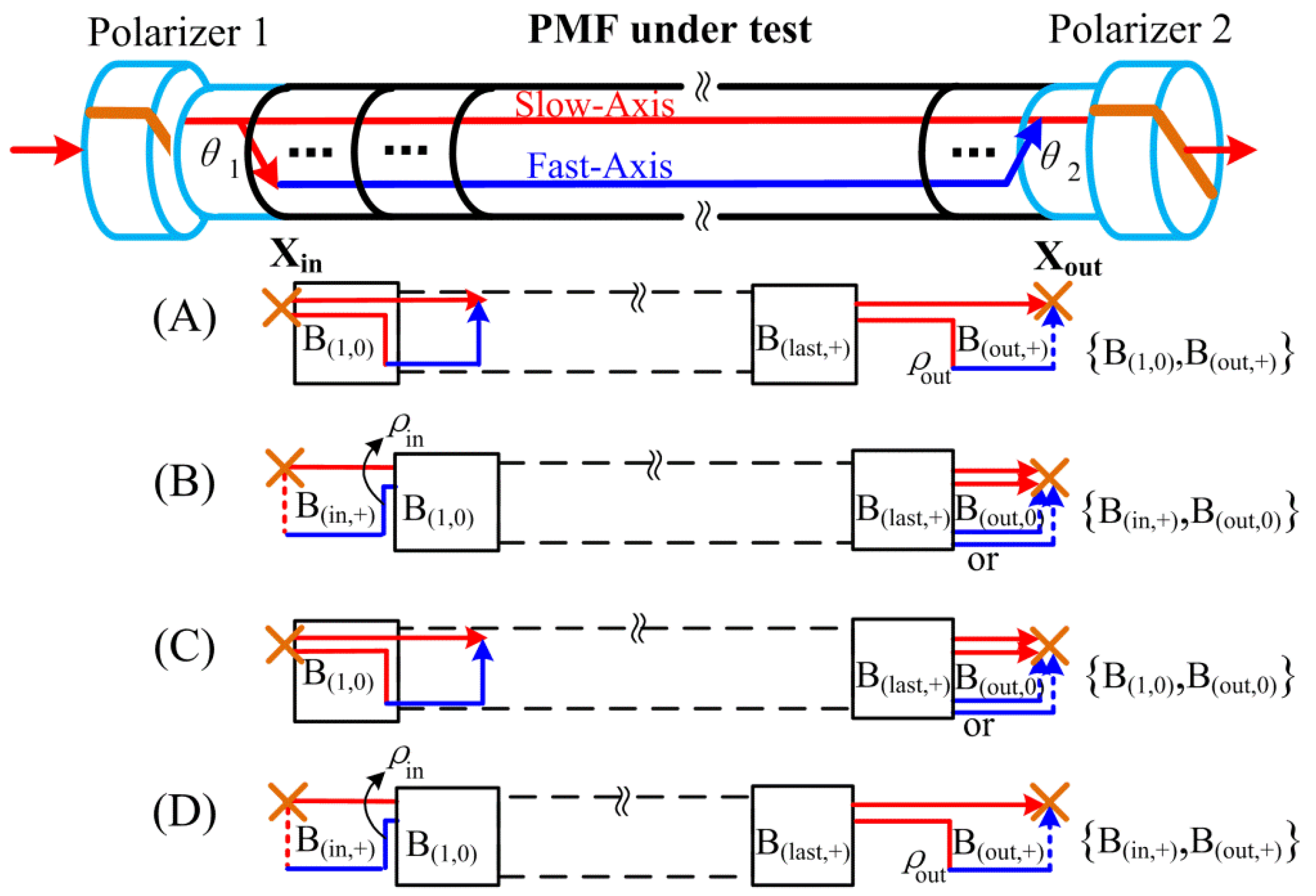
2.2.2. Classifications and General Formulas
3. Experimental Results
3.1. Theoretical Estimation
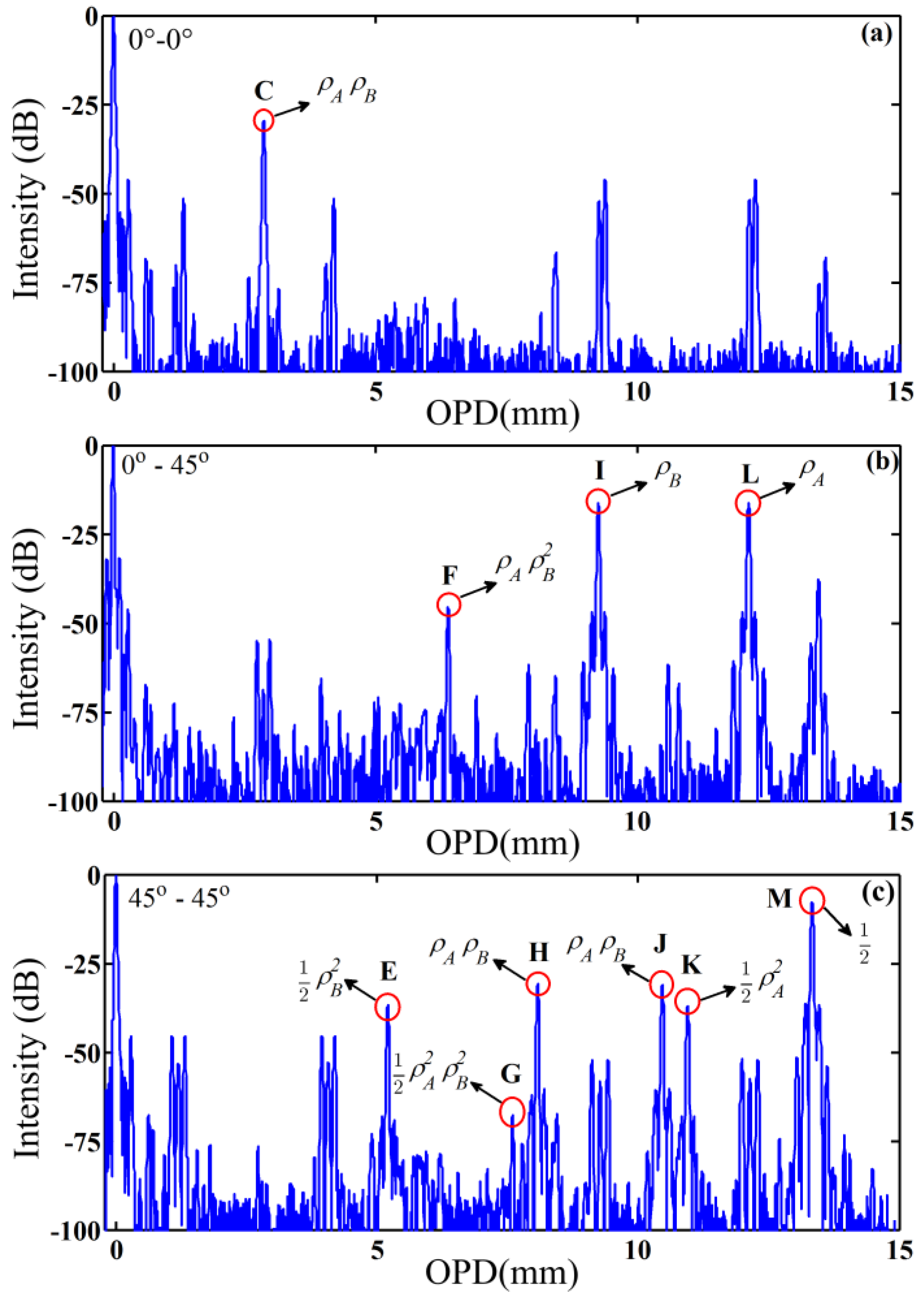
3.2. Identification of HOI and Results
4. Discussions
5. Conclusions
Acknowledgments
Author Contributions
Conflicts of Interest
References
- Noda, J.; Okamoto, K.; Sasaki, Y. Polarization-maintaining fibers and their applications. J. Lightwave Technol. 1986, 4, 1071–1089. [Google Scholar] [CrossRef]
- Kim, J. An all fiber white light interferometric absolute temperature measurement system. Sensors 2008, 8, 6825–6845. [Google Scholar] [CrossRef]
- Okamoto, K.; Hosaka, T.; Edahiro, T. Stress analysis of optical fibers by a finite element method. IEEE J. Quantum. Elect. 1981, 17, 2123–2129. [Google Scholar] [CrossRef]
- Dong, Y.; Xu, P.; Zhang, H.; Lu, Z.; Chen, L.; Bao, X. Characterization of evolution of mode coupling in a graded-index polymer optical fiber by using brillouin optical time-domain analysis. Opt. Express 2014, 22, 26510–26516. [Google Scholar] [CrossRef] [PubMed]
- Yang, J.; Yuan, Y.; Zhou, A.; Cai, J.; Li, C.; Yan, D.; Huang, S.; Peng, F.; Wu, B.; Zhang, Y.; et al. Full Evaluation of Polarization Characteristics of Multifunctional Integrated Optic Chip with High Accuracy. J. Lightwave Technol. 2014, 32, 3641–3650. [Google Scholar]
- Takada, K.; Chida, K.; Noda, J. Precise method for angular alignment of birefringent fibers based on an interferometric technique with a broadband source. Appl. Opt. 1987, 26, 2979–2987. [Google Scholar] [CrossRef] [PubMed]
- Takada, K.; Noda, J.; Okamoto, K. Measurement of spatial distribution of mode coupling in birefringent polarization-maintaining fiber with new detection scheme. Opt. Lett. 1986, 11, 680–682. [Google Scholar] [CrossRef] [PubMed]
- Yuan, Y.; Li, C.; Yang, J.; Zhou, A.; Liang, S.; Yu, Z.; Wu, B.; Peng, F.; Zhang, Y.; Liu, Z.; et al. Simultaneous evaluation of two branches of a multi-functional integrated optic chip with an ultra-simple dual-channel configuration. Photon. Res. 2015, 3, 115–118. [Google Scholar] [CrossRef]
- Bohm, K.; Petermann, K.; Weidel, E. Performance of Lyot depolarizers with birefringent single-mode fibers. J. Lightwave Technol. 1983, 1, 71–74. [Google Scholar] [CrossRef]
- Wang, L.; Fang, N.; Wu, C.; Qin, H.; Huang, Z. A fiber optic PD sensor using a balanced Sagnac interferometer and an EDFA-Based DOP Tunable fiber ring laser. Sensors 2014, 14, 8398–8422. [Google Scholar] [CrossRef] [PubMed]
- Cordova, A.; Patterson, R.; Goidner, E.; Rozelle, D. Interferometric fiber optic gyroscope with inertial navigation performance over extended dynamic environments. In Proceedings of the SPIE 2070 Fiber Optic and Laser Sensors XI, Boston, MA, USA, 7 September 1993; pp. 164–180.
- Chen, S.; Giles, I.; Fahadiroushan, M. Quasi-distributed pressure sensor using intensity-type optical coherence domain polarimetry. Opt. Lett. 1991, 16, 342–344. [Google Scholar] [CrossRef] [PubMed]
- Gauthier, R. Polarization-maintaining distributed fiber-optic sensor: Software elimination of second-order (ghost) coupling points. Appl. Opt. 1995, 34, 1744–1748. [Google Scholar] [CrossRef] [PubMed]
- Song, D.; Wang, Z.; Chen, X.; Zhang, H.; Liu, T. Influence of ghost coupling points on distributed polarization cross-talking measurements in high birefringence fiber and its solution. Appl. Opt. 2015, 54, 1918–1925. [Google Scholar] [CrossRef] [PubMed]
- Choi, W.; Jo, M. Accurate evaluation of polarization characteristics in the integrated optic chip for interferometric fiber optic gyroscope based on path-matched interferometry. J. Opt. Soc. Korea 2009, 13, 439–444. [Google Scholar] [CrossRef]
- Maheshwari, M.; Tjin, S.C.; Asundi, A. Efficient design of Fiber Optic Polarimetric Sensors for crack location and sizing. Opt. Laser Technol. 2015, 68, 182–190. [Google Scholar] [CrossRef]
- Li, C.; Yang, J.; Yuan, Y.; Zhou, A.; Yan, D.; Chai, J.; Liang, S.; Hou, L.; Wu, B.; Peng, F.; et al. A differential delay line for optical coherence domain polarimetry. Meas. Sci. Technol. 2015, 26. [Google Scholar] [CrossRef]
- Szafraniec, B.; Feth, J.; Bergh, R.; Blake, J. Performance improvements in depolarized fiber gyros. In Proceedings of the SPIE 2510 Fiber Optic and Laser Sensors XI, Munich, Germany, 19–23 June 1995; pp. 37–48.
- Tsubokawa, M.; Higashi, T.; Sasaki, Y. Measurement of mode couplings and extinction ratios in polarization-maintaining fibers. J. Lightwave Technol. 1989, 7, 45–50. [Google Scholar] [CrossRef]


| Interferogram | Position Meaning | Interferogram Meaning | Position (mm) | Normalized Intensity/Error (dB) | Order N | |||
|---|---|---|---|---|---|---|---|---|
| 0°–0° | 0°–45° | 45°–0° | 45°–45° | |||||
| 0 | 1 | 0 | 0 | 0 | 0 | 0 | ||
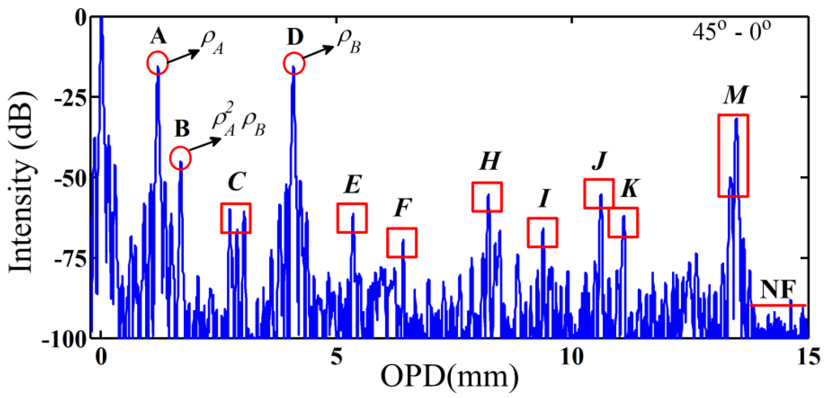
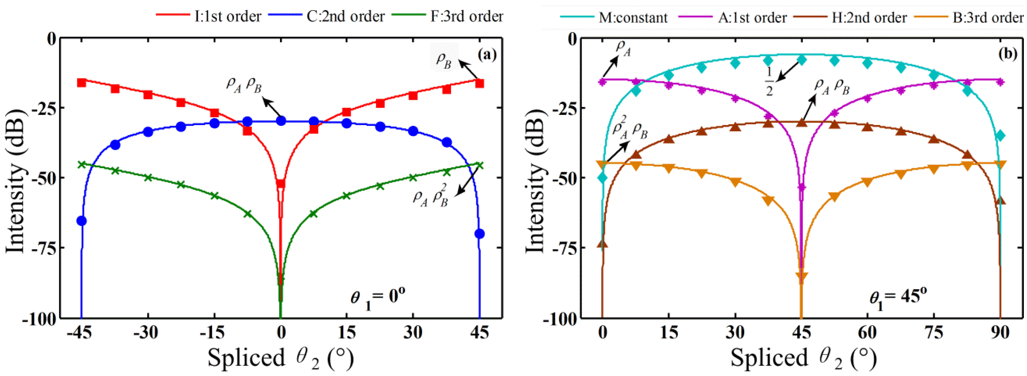
| M | 13.33 | <−70 | <−50 | <−50 | −7.8/1.8 | 0th | ||
| A | 1.22 | <−70 | <−70 | −15.6/0.7 | <−50 | 1st | ||
| D | 4.09 | <−70 | <−70 | −15.7/0.7 | <−50 | |||
| I | 9.27 | <−50 | −16.5/1.5 | <−70 | <−50 | |||
| L | 12.12 | <−50 | −16.3/1.4 | <−70 | <−50 | |||
| C | 2.87 | −29.7/0.2 | <−60 | <−60 | <−70 | 2nd | ||
| E | 5.21 | <−70 | <−70 | <−70 | −36.7/0.7 | |||
| H | 8.08 | <−70 | <−70 | <−70 | −30.6/0.7 | |||
| J | 10.47 | <−70 | <−70 | <−70 | −31.0/1.1 | |||
| K | 10.95 | <−70 | <−70 | <−70 | −36.9/1.1 | |||
| B | 1.70 | <−70 | <−70 | −45.1/0.3 | <−70 | 3rd | ||
| F | 6.38 | <−70 | −45.7/0.8 | <−60 | <−70 | |||
| G | 7.60 | <−70 | <−70 | <−70 | −67.7/1.9 | 4th | ||
© 2016 by the authors; licensee MDPI, Basel, Switzerland. This article is an open access article distributed under the terms and conditions of the Creative Commons by Attribution (CC-BY) license (http://creativecommons.org/licenses/by/4.0/).
Share and Cite
Li, C.; Yang, J.; Yu, Z.; Yuan, Y.; Zhang, J.; Wu, B.; Peng, F.; Yuan, L. High-Order Interference Effect Introduced by Polarization Mode Coupling in Polarization—Maintaining Fiber and Its Identification. Sensors 2016, 16, 419. https://doi.org/10.3390/s16030419
Li C, Yang J, Yu Z, Yuan Y, Zhang J, Wu B, Peng F, Yuan L. High-Order Interference Effect Introduced by Polarization Mode Coupling in Polarization—Maintaining Fiber and Its Identification. Sensors. 2016; 16(3):419. https://doi.org/10.3390/s16030419
Chicago/Turabian StyleLi, Chuang, Jun Yang, Zhangjun Yu, Yonggui Yuan, Jianzhong Zhang, Bing Wu, Feng Peng, and Libo Yuan. 2016. "High-Order Interference Effect Introduced by Polarization Mode Coupling in Polarization—Maintaining Fiber and Its Identification" Sensors 16, no. 3: 419. https://doi.org/10.3390/s16030419