1. Introduction
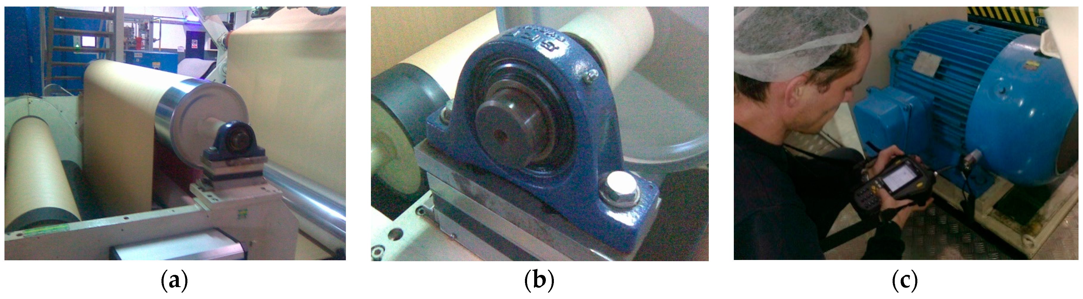
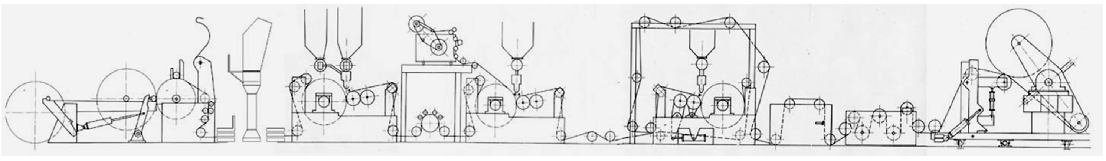
The production processes in the packaging materials industry has to be very efficient and cost-effective. These processes usually take place under extreme conditions and high speeds that require a high level of both reliability and safety. In order to further increase its competitiveness the packaging materials industry needs to deploy advanced maintenance strategies and solutions for improved reliability of its production equipment, as well as safety of its production processes. Total Productive Maintenance (TPM) is one such strategy that is usually performed at the plant level. As such, it plays an increasingly important role in order to achieve a reliable, safe, and efficient operation of production machines. TPM aims to optimize the entire maintenance program and define optimal measures to be implemented on each of the machines. Manufacturing of paper-based packaging materials usually includes three key production processes which are printing, laminating, and slitting, in that order. All of these processes take place under extreme conditions and high speeds of up to 1000 m/min that requires a high level of reliability and safety. Rollers, together with their supporting bearings and electric motors, as shown in
Figure 1 and
Figure 2, are the most common components of these production machines. Bearings operate under high loading and severe conditions and their faults represent one of the foremost causes of failures.
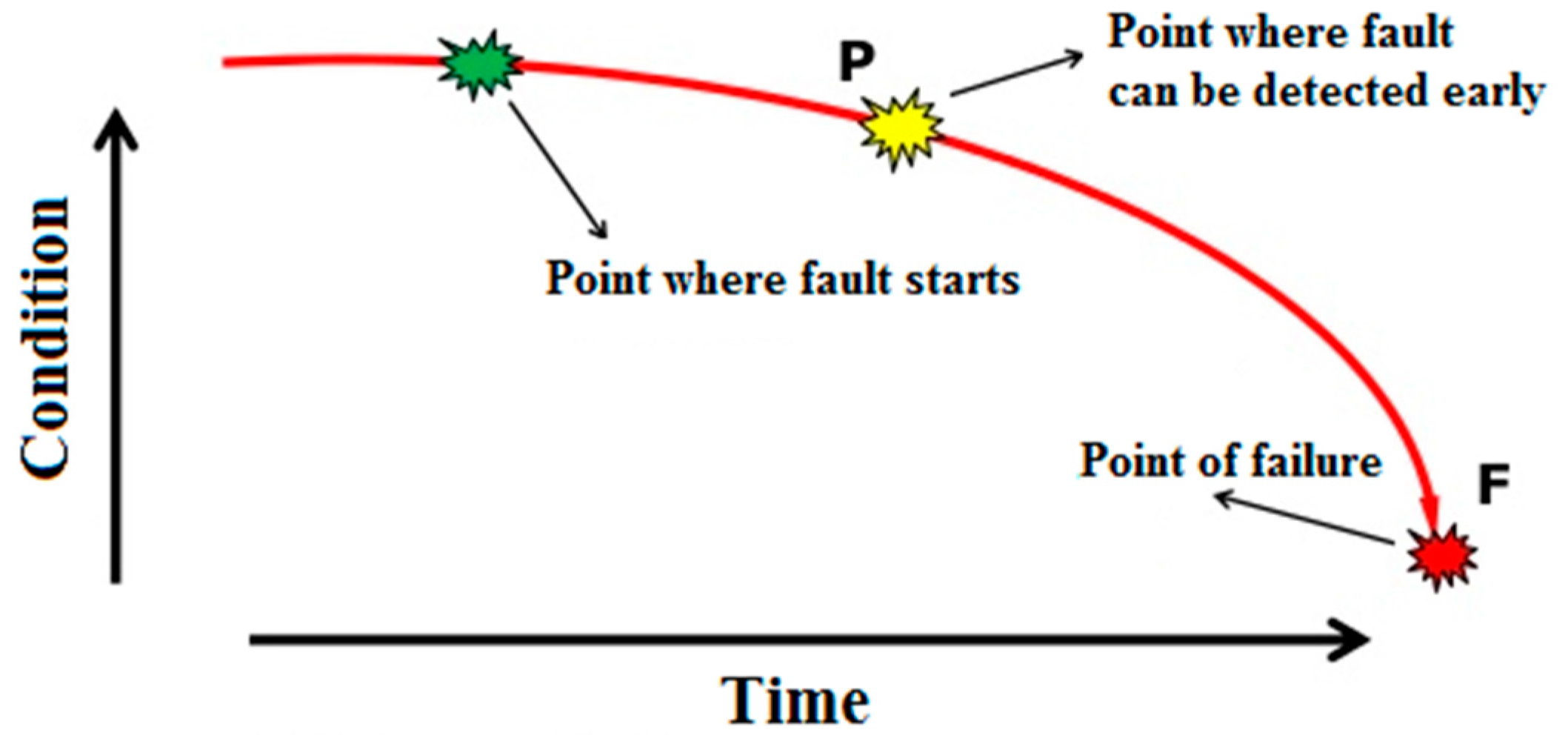
As shown in
Figure 3, bearing faults often occur gradually. Defective bearings generate various forces causing high amplitude vibrations. Therefore, it is very important to avoid deteriorating conditions, degraded reliability, and unexpected failures of bearings. Based on TPM analysis performed on the laminator at the Tetra Pak packaging materials plant in Gornji Milanovac, Serbia it has been concluded that, for most of bearings, a regular check of vibration levels every two weeks by a portable, handheld data collector and analyzer can ensure their reliable operation and early detection of bearing faults [
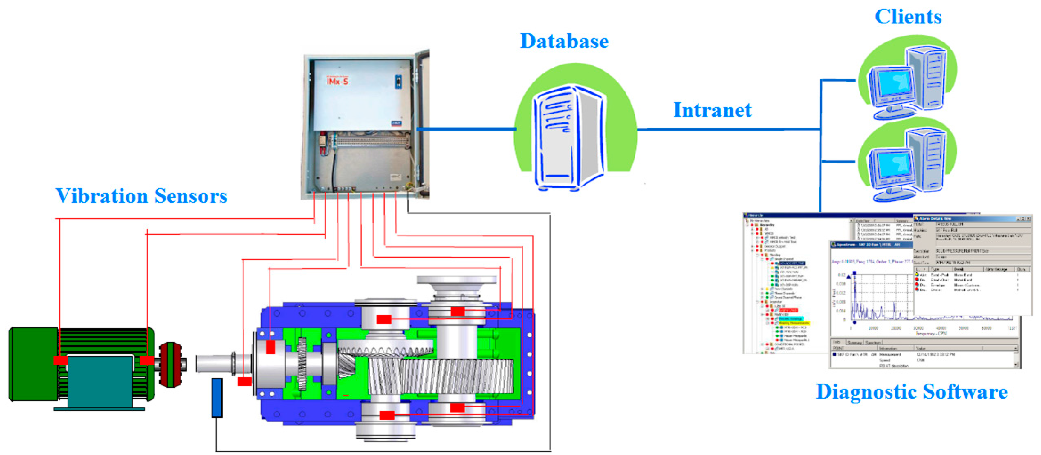
1]. However at a few critical points it has been proposed to do more frequent checks that becomes resource-demanding and not so optimal anymore. Therefore, installation of an online vibration monitoring system including deployment of an automated technique for early fault detection and diagnosis (FDD) in bearings is needed. Such a system saves the time of maintenance technicians and enables an objective, reliable, and faster detection and diagnosis of bearing faults. Since vibration sensors and data acquisition systems are already available in the market, the Tetra Pak plant has designed an online vibration monitoring system as presented in
Figure 4. The online vibration sensors will continually monitor the condition of a few critical bearings whose failure in the past caused stoppages of the entire production for a couple of hours, resulting in a significant loss. At the same time, the plant also initiated development of a new automated technique for early FDD in bearings to be tested and potentially deployed in this plant once all the equipment is installed. This paper focuses on development of such a technique.
Even though there are some techniques for FDD in bearings based on force measurements [
2] most of them that have emerged in recent years are based on vibration signal analysis. Generally, an FDD can be decomposed into three steps: data acquisition, feature extraction, and classification. An effective feature extraction as the key step represents a mapping of vibration signals from their original measured space to the feature space which contains more valuable information for FDD. Even though time-domain features, e.g., peak, mean, root mean square, and variance, have also been employed as input features to train a bearing FDD classifier, the fast Fourier transform (FFT) is the most widely applied and established feature extraction methods [
3]. However, the techniques based on FFT are not suitable for analysis of non-stationary signals. Since vibration signals often contain non-stationary components, for a successful FDD it is very important to reveal such information as well. Thus, a supplementary technique for non-stationary signal analysis is necessary. Time-frequency techniques, e.g., the Wigner-Ville distribution (WVD) [
4] and the short-time Fourier transform (STFT) [
5] also have their own disadvantages. The WVD bilinear characteristic causes interference terms in the time-frequency domain while the STFT results in a constant resolution for all frequencies having in mind that it uses the same window size for the analysis. The wavelet transform resolves all these deficiencies. It ensures a good frequency resolution and low time resolution for low-frequency components while, for high-frequency components, it provides low-frequency resolution and good time resolution. Therefore, the wavelet transform is widely applied in the vibration signal analysis and feature extraction for bearing FDD [
6,
7]. Classification, as the next step, directly depends on previously extracted features,
i.e., there is no classifier which can make up for the information lost during the feature extraction. As in the case of the feature extraction, we can come across a wide range of classifiers used for FDD in bearings. The classifiers based on artificial neural networks [
8,
9,
10] and fuzzy logic [
11,
12] demonstrated a very reliable classification. However, the disadvantage of the mentioned classification techniques is that they require the availability of a very large training set. They also have a large number of parameters to be selected and adjusted in order to obtain acceptable results [
13]. Therefore, there is a strong need to make the classification process simpler, faster, and accurate using as few features and parameters as possible.
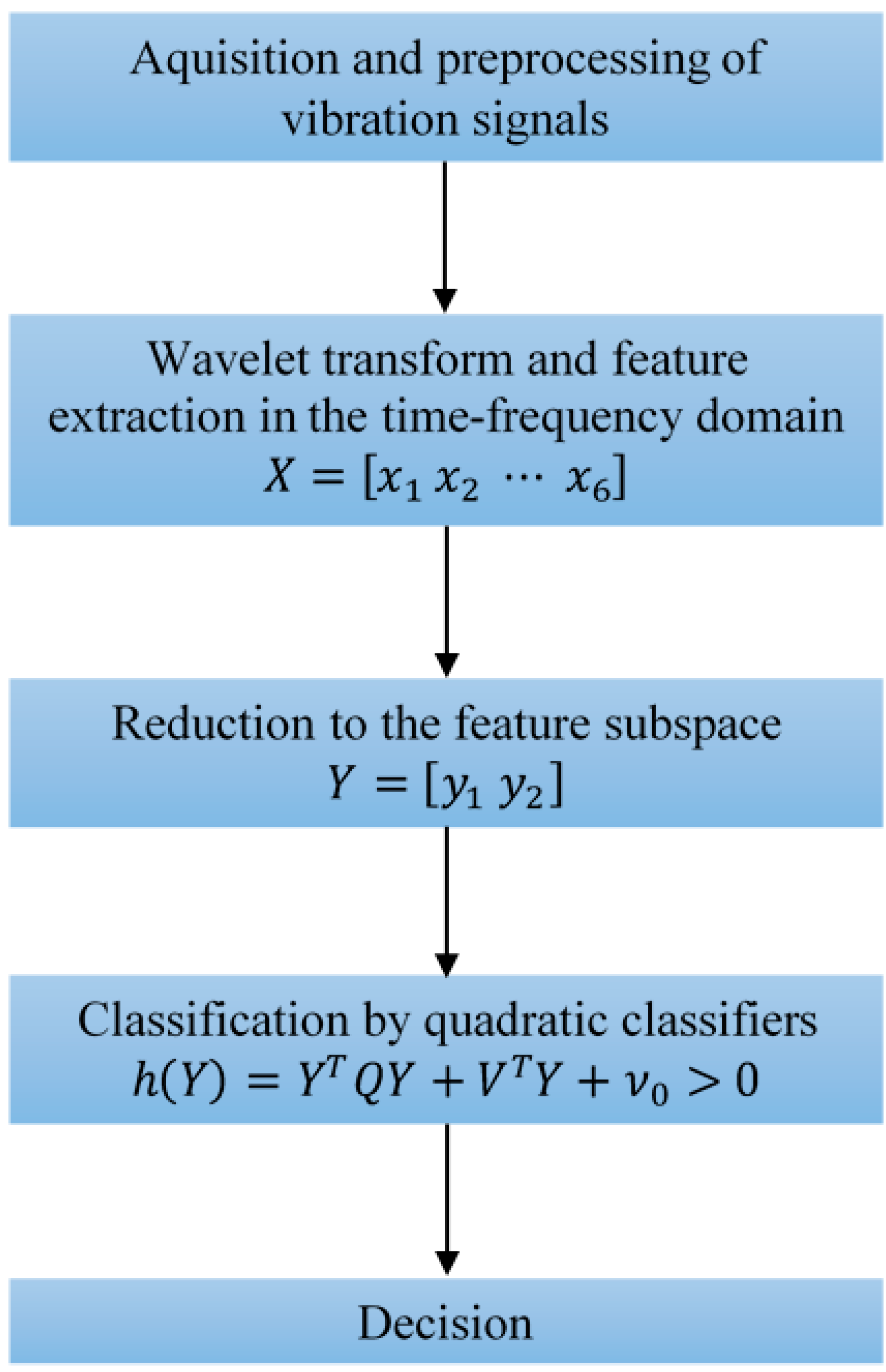
In this paper a new technique for early FDD is proposed. As shown in
Figure 5 it has a few steps. The first one is acquisition of signals, as well as their preprocessing, which includes normalization and segmentation. The vibration signals are normalized to zero mean and unit variance in order to minimize impact of their magnitude on accuracy. Even though the signals are recorded in real-time at the sampling frequency of 12,000 Hz they are further processed in subsequent segments of 1024 samples each, which enables faster execution of the entire technique and also, at the same time, captures all the fault frequencies of interest. In the next step, and after the wavelet transform of vibration signals, six representative features,
i.e., the standard deviation of the wavelet coefficients in six sub-bands, are extracted in the time-frequency domain. The standard deviation is used as a measure of the average and relative energy in each sub-band since the vibration signals were previously normalized to zero mean and unit variance. In the third step the feature space dimension is optimally reduced to two using scatter matrices and keeping in mind their rank. The dimension reduction to two also enables much better visualization of classification results. In the fourth step, a total of three quadratic classifiers are designed [
14], one for detection and the other two for diagnosis of bearing faults. Based on the classification results in the final step a decision about bearing state is made. Using this new approach, the overall complexity of FDD is decreased and, at the same time, a very high accuracy maintained compared with already available techniques which deploy more complex training algorithms.
2. Materials and Methods
2.1. Acquisition and Preprocessing of the Vibration Signals
Before deployment of the new technique into a real production environment, its capability was tested using the vibration data obtained from the CWRU Bearing Data Center [
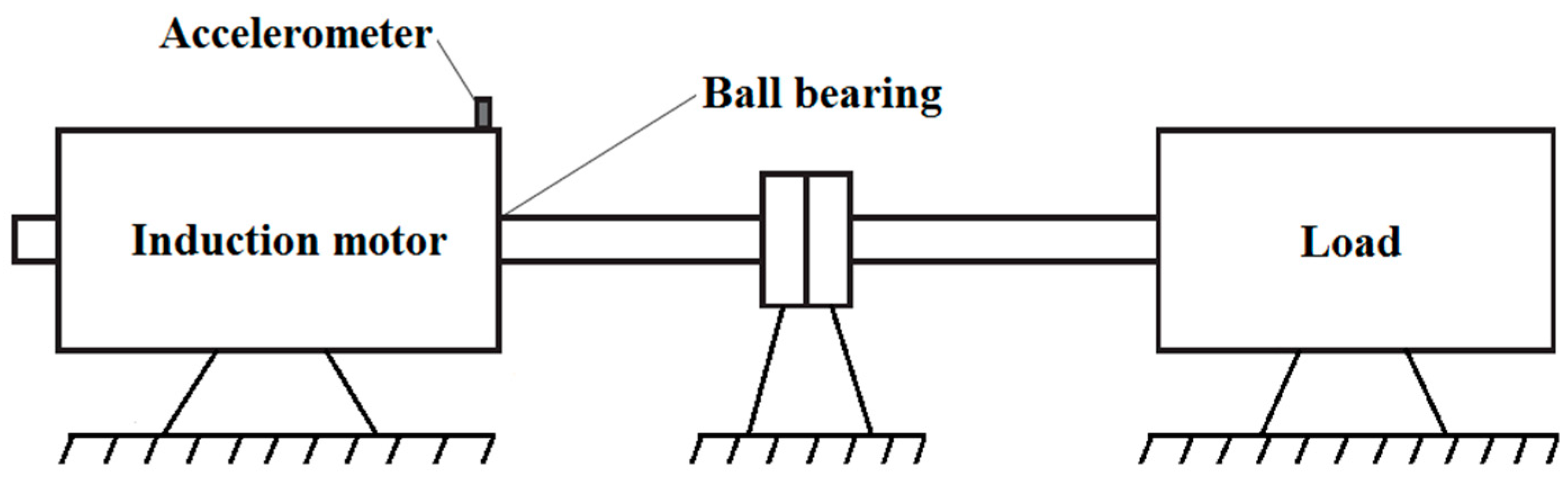
11]. This vibration data has become a standard reference in the field of FDD in bearings and enables an objective comparison of different techniques developed so far. A ball bearing SKF 6205-2RS JEM (SKF, Gothenburg, Sweden) was installed in a motor-driven system as presented in
Figure 6. The bearing fault frequencies as a multiple of shaft speed are as follows [
15]:
Ball pass frequency, outer race: 5.415;
Ball pass frequency, inner race: 3.585;
Fundamental train frequency (cage speed): 0.3983; and
Ball (roller) spin frequency: 2.357.
An accelerometer with a bandwidth up to 5000 Hz and a 1 V/g output was used to acquire the vibration signals from the bearing. Acceleration was measured in the vertical direction on the housing of the drive-end bearing. The sampling rate of 12,000 Hz is sufficient, keeping in mind that the frequency content of interest does not exceed 5000 Hz. In total, four sets of data were obtained and used:
Under normal conditions;
With inner race faults;
With ball faults; and
With outer race faults.
The faults with diameter from 0.007 to 0.40 inches and depth of 0.011 inches were introduced separately at the bearing elements. The bearing was tested under different loads,
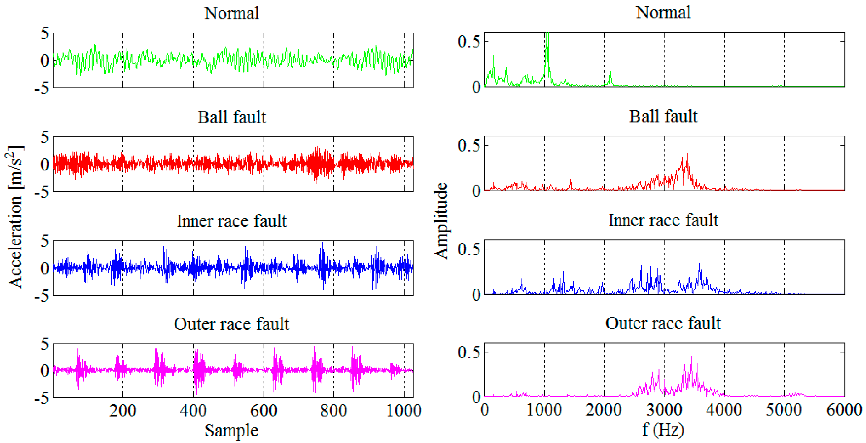
i.e., 0, 1, 2, and 3 hp, while the shaft rotating speeds were 1730, 1750, 1772, and 1797 rpm. Only the smallest fault diameter was selected for this study since we were interested in an early FDD. In order to make the entire technique more robust and less dependent on magnitude, the recorded vibration signals were normalized to zero mean and unit variance. The vibration signals collected from each of the four different conditions are divided into 256 segments of 1024 sample each, as shown in
Figure 7. The segment length was chosen such that it enables real-time implementation of the technique in an industrial environment and also capture the bearing fault frequencies of interest. In total 1024 segments were used, 512 for design and 512 for testing of the new technique for early FDD in bearings. Based on the frequency spectra given in
Figure 7 we can notice that it is easy to detect a bearing fault while its diagnosis is not so straightforward.
2.2. Wavelet Transform
As we already know, a signal can be represented as linear combination of basic functions. A unit impulse function with limited power is limited and non-zero mean is the basic function in the time domain. In the frequency domain, the role of a basic function is assigned to the sinusoidal function with infinite power and zero mean. When using the wavelet transform to transform the signal from the time domain to the time-frequency domain, the basic function is the wavelet. The wavelet is a function of limited power and zero mean [
16], and for which the following is valid:
The wavelet can be moved in time for
samples and scaled by the so-called dilation parameter
. In such a case it is given by:
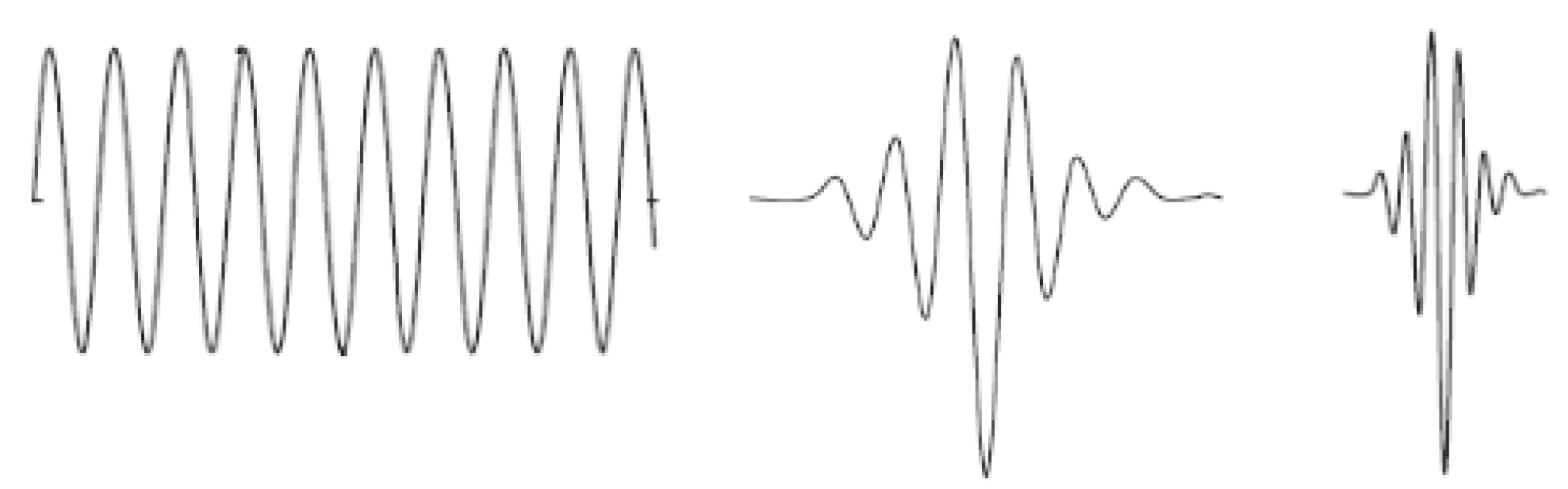
If the dilation parameter changes, the basic wavelet (
) changes its width and, thus, spreads (
) or contracts (
) in the time domain as shown in
Figure 8. In the analysis of non-stationary signals, such a possibility represents a significant advantage, considering the fact that wider wavelets are useful for extraction of slower changes,
i.e., low-frequency components, while narrower wavelets are useful for extraction of faster changes,
i.e., high-frequency components. Following the selection of
and
it is possible to transform segments of the signal
of
samples, and calculate the wavelet transform coefficients in the following way:
Only those frequencies which are within the wavelet frequency band are extracted, i.e., the signal is filtered by the wavelet Using the wavelet coefficients, the original signal can be reconstructed that is inverse wavelet transform. It is also possible to independently reconstruct both filtered and rejected parts of the signal by the wavelet using the so-called detail and approximation coefficients, respectively, which are, of course, a function of the transformation coefficients
Parameters and can be continuous. However this is not so practical since the signal can be transformed and reconstructed by using smaller number of wavelets, i.e., a limited number of discrete values of and . It is known as the discrete wavelet transform (DWT) where parameters and are the powers of 2 and, in that case, frequency bands do not overlap each other. The dilation parameter a, as the power of 2, at each subsequent higher level of transformation, doubles in value in comparison to the value from the previous level. Thus, the signal frequency band from the previous level is split into two halves at every next level, into a higher band which contains finer changes, or details, and a lower band, which is an approximation of the signal from the previous level. This technique is known as the wavelet packet decomposition. We apply the five-level wavelet decomposition of the vibration signals recorded with a sampling frequency of 12,000 Hz that results into the following six frequency sub-bands 0–187.5 Hz, 187.5–375 Hz, 375–750 Hz, 750–1500 Hz, 1500–3000 Hz, and 3000–6000 Hz. After the wavelet decomposition, the standard deviation of the obtained wavelet coefficients in each sub-band is extracted as representative feature that results into a six-dimensional feature vector for each of the analyzed segments.
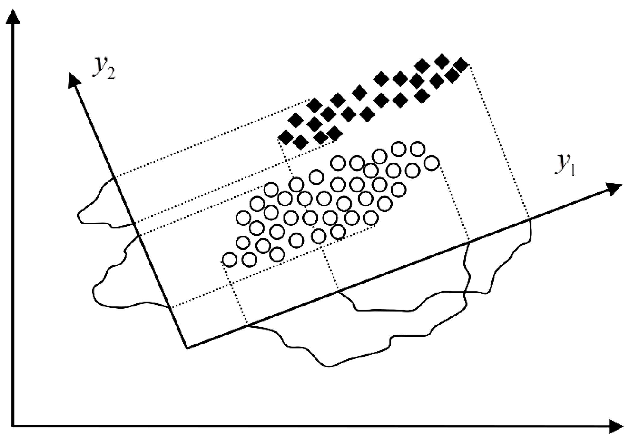
2.3. Dimension Reduction in the Feature Space
Let a feature vector
be transformed into
where
is an
n-dimensional transformation matrix. Mapping of
into the space which is made up by the eigenvectors
of its covariance matrix
is known as the principal component analysis (PCA) [
17]. When reducing the feature space dimension using the PCA the performance of each feature
is characterized by its eigenvalue
, respectively. Thus, by rejecting features, we should first reject those with the smallest eigenvalue. In other words, the rejected features have the smallest variance in the new feature space. In the case shown in
Figure 9 where the dimension is reduced from two to one, the mapped feature
would be rejected based on the PCA as less informative even though it has better discriminatory potential than
.
Unlike the PCA, the dimension reduction based on scatter matrices [
14] is more interesting in this work since it also takes into consideration classification as one of the purposes of the dimension reduction. Let
be the number of classes to be classified and
and
their mean vectors and covariance matrices. Then the within-class scatter matrix is given as:
while the between-class scatter matrix is defined as:
is the joint vector of mathematical expectation for all the classes together,
i.e.:
In addition the mixed scatter matrix can be given as:
Then the problem of dimension reduction is reduced to the identification of the
transformation matrix
which maps the
-dimensional vector
into the
-dimesnional random vector
and also maximizes the criteria
. This criteria is invariant to non-singular linear transformations and results into transformation matrix that takes the following form:
where
,
are the eigenvectors of
which correspond to its
greatest eigenvalues. The dimension reduction based on scatter matrices applied to the case shown in
Figure 9 would result into selection of the mapped feature
. Obviously it is a much better choice than
selected by the PCA in terms of more accurate classification as the main goal of the dimension reduction. Since the rank of
is at most
(
is the number of classes) we can reduce the dimensionality to, at most,
. Having in mind that in our application we are going to deal with a maximum of three classes the dimension will be reduced to two.
2.4. Design of Quadratic Classifiers
Following the dimension reduction to two, as a next step we design quadratic classifiers in order to detect and diagnose different bearing faults. Quadratic classifiers are known as very robust solutions to the classification problems whose statistical features change over time [
14]. In addition, they also provide visual insight into the classification problem. Quadratic classifiers to be designed in the two-dimensional feature subspace
can be defined by the following equation:
The matrix
, vector
and scalar
are the unknowns to be optimally determined. Equation (9) can be represented in a linear form as:
In order to achieve as large as possible between-class and as short as possible within-class scattering we have selected the following function as the optimization criterion [
14]:
where
and
are probabilities and:
and
are the mean vectors and covariance matrices, respectively, of the vector
for each of classes which should be classified. After optimization of the function
, the optimal vector
and, thus, the optimal matrix
and vector
, gets the following form:
while the optimal scalar is:
which finishes the design procedure of quadratic classifiers. Based on the designed classifiers a decision about bearing state can be made as it will be demonstrated in the next section.
3. Results and Discussion
In order to extract representative features, and before we apply the wavelet transform, it is necessary to choose both the basic wavelet type and the number of resolution levels into which the vibration signal segments will be decomposed. After analysis of a few types of the basic wavelets, the fourth-order Daubechies wavelet was selected. It demonstrated the best discriminatory potential and resulted into the fault detection accuracy that was higher by 2%–5% compared with other basic wavelets. This type of wavelet has very good localizing properties in the time-frequency domain due to its shape and frequency characteristics [
18] and, thus, is very suitable for this particular application. Following the five-level wavelet decomposition, the standard deviation of the obtained wavelet coefficients in each sub-band is extracted as representative feature in the time-frequency domain. Note that the standard deviation is used here to quantify the average and relative energy in each sub-band because the vibration signals were previously normalized to zero mean and unit variance. In total, six features were extracted for each of 1024 analyzed segments. So now each original segment recorded in the time domain is represented by its feature vector
that consists of standard deviations of the wavelet coefficients in six sub-bands. The extracted features for all four classes together with their statistics are given in
Table 1.
Obviously, in the presence of a bearing fault there is a shift in energy in the vibration signals from lower to higher sub-bands. In
Figure 7 and
Figure 10, and
Table 1, it can be noticed that most of the extracted features have a certain potential for the fault detection but not for the fault diagnosis. Therefore it is necessary to find their optimal combination in order to achieve a better separability between different classes of bearing condition. That is usually done by a mapping of the existing feature space into a new one whose dimension can be reduced without any significant loss of information, which makes the classification process much simpler. Although the PCA is one of the most widely used techniques for reduction of the feature space dimension in this paper we apply the technique based on scatter matrices [
14] since it is more suitable for classification problems, as described in
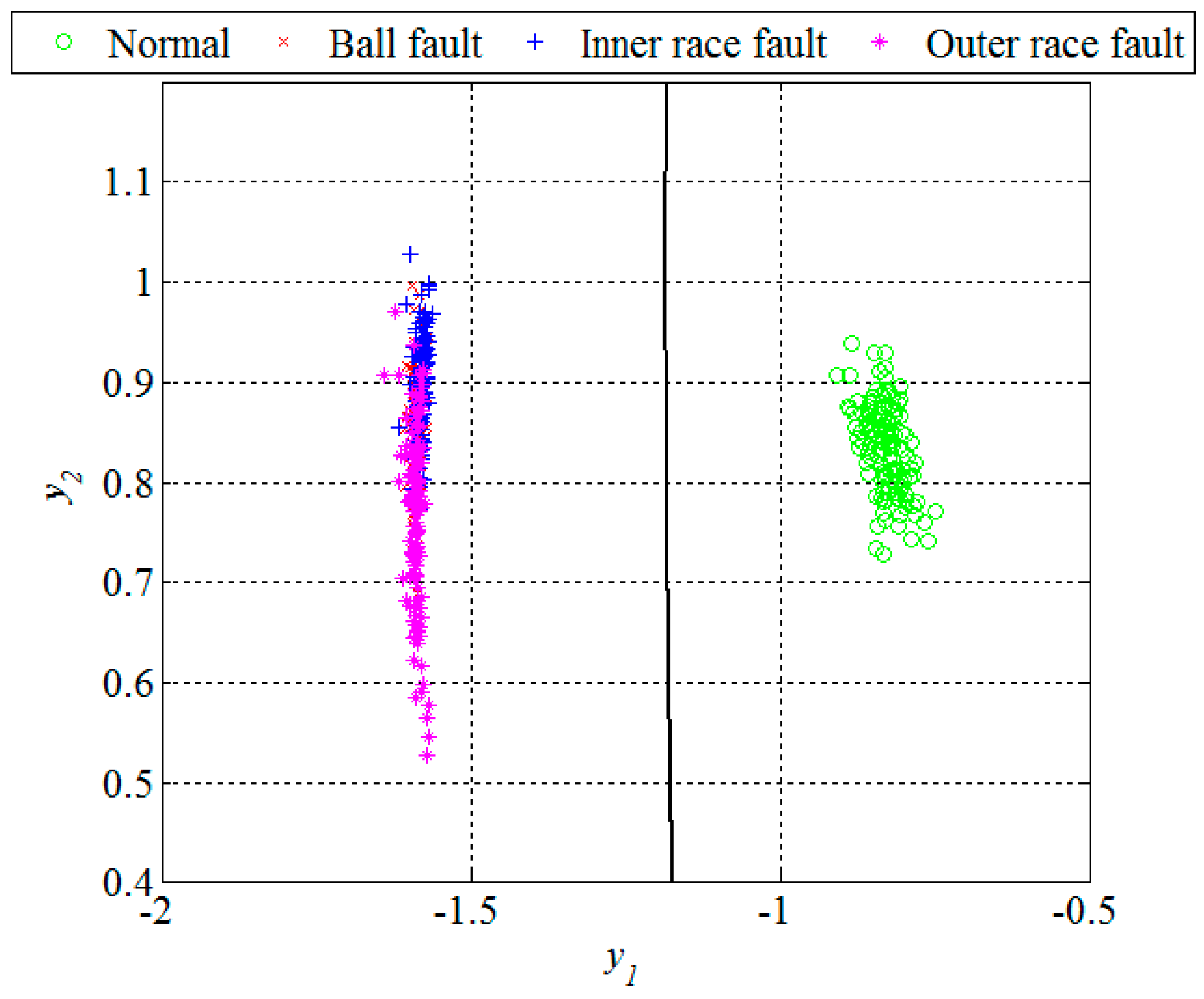
Section 2.3. At first, we reduce the feature space dimension to enable the fault detection and then repeat the same procedure in order to diagnose the detected fault as shown in
Figure 11 and
Figure 12. In this way separabilty between different classes is increased compared with
Figure 10. After the dimension reduction, we designed suitable quadratic classifiers following the procedure described in
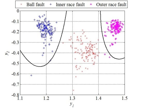
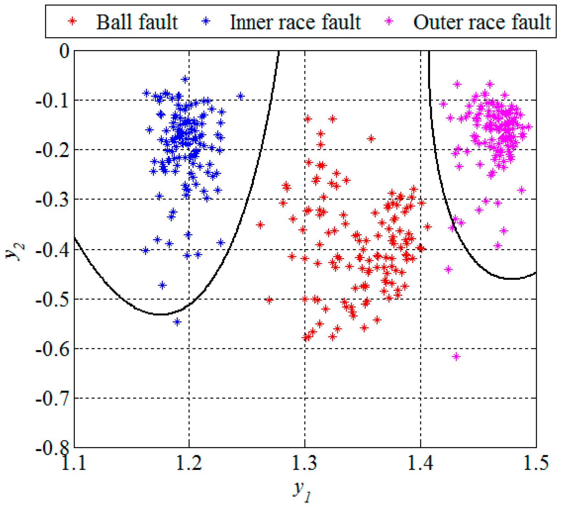
Section 2.4, which is also the last step in design of the new technique for early FDD. The first quadratic classifiers shown in
Figure 11 separates normal from faulty condition, i.e., performs the fault detection, while the other two quadratic classifiers shown in
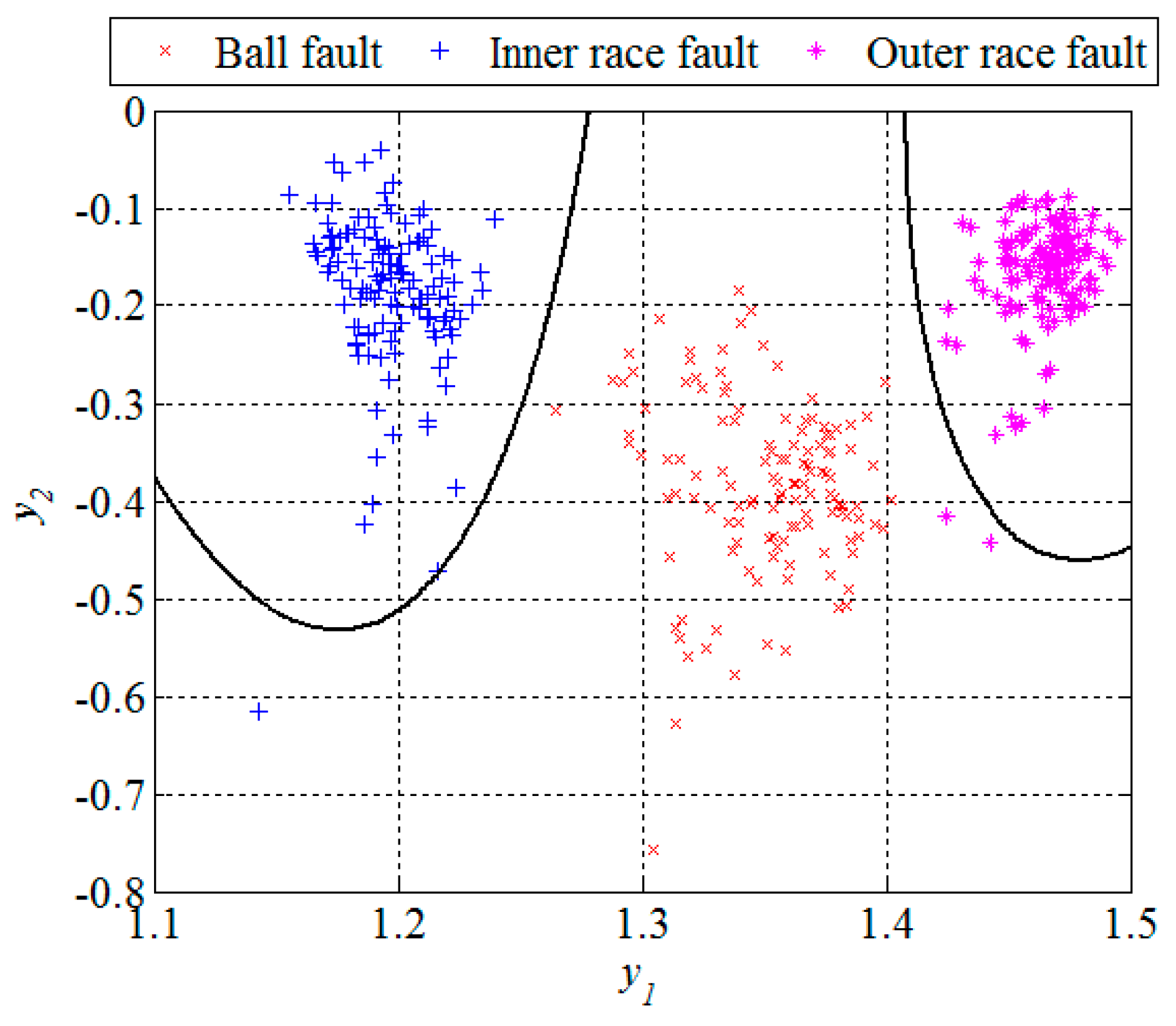
Figure 12 are able to separate all three different bearing faults from each other and, thus, perform the fault diagnosis.
The classification results can be given by a confusion matrix which compares the classification results with ground truth information, as is shown in
Table 2. Based on
Figure 12 and the confusion matrix, we can conclude that all the segments from the ball fault class were correctly classified. However, the remaining two classes contained in total three segments which were incorrectly classified,
i.e., classified as they belong to the ball fault class. Statistical performances, such as sensitivity, specificity, and accuracy of the new technique are estimated based on these classification results. The sensitivity is defined as a ratio between the number of correctly classified segments and the total number of the segments for each of the classes separately. The specificity is also calculated for each of these three classes separately and represents the ratio between the number of correctly classified features of the other two classes and the total number of the segments of these two classes. The accuracy is calculated as the ratio between the total number of correctly classified segments and the total number of the segments in all three classes together. For segments of the design set, the accuracy of 99.2 was achieved, while other statistical performances are shown in
Table 3.
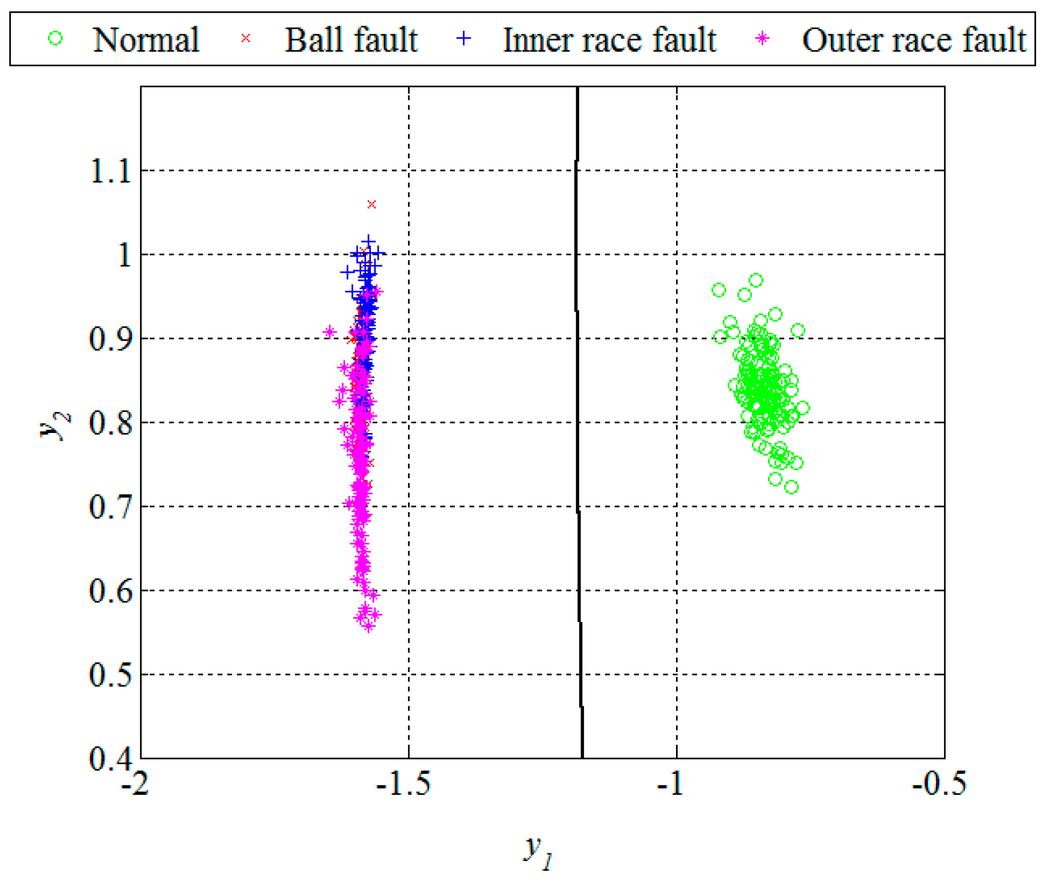
Unlike in the previous two figures, where the design set of 512 segments is shown,
Figure 13 and
Figure 14 show the remaining set of 512 segments used to test the performance of the new technique for early FDD as well. The confusion matrix and statistical performances for the testing set are given in
Table 4 and
Table 5, respectively. The total accuracy of the new technique for early FDD in bearings is 98.9%. Usually, quadratic classifiers are robust and do not result in overtraining when the number of estimated parameters is much less than the number of analyzed samples, as in this case. However, it is a good practice to cross-validate these quadratic classifier in order to ensure its stability. A five-fold cross-validation was performed and it resulted in cross-validation loss,
i.e., the error of the out-of-fold samples, of 1.4%. Even though it is slightly higher than the classification error of 1.1% it gives a confidence that the classifier is reasonably stable.
Taking into account the results of other techniques tested on the same vibrations signals [
18], the new technique demonstrated very good performance, which is either better than, or comparable to, other available techniques which usually deploy much more complex algorithms, as can be seen from
Table 6. In addition, in this work only the segments with the smallest fault diameter were used because we were interested in incipient FDD. It should also be emphasized that the vibration signals were normalized before further processing. In that way we managed to overcome one of the main disadvantages of other techniques in terms of application in a real production environment since most of them also depend on the amplitude of the vibration signals. However, the amplitude has been found as unreliable in real applications since it varies even with healthy bearings, e.g., depending on their load. The vibration data obtained from the CWRU Bearing Data Center have quite a high signal to noise ratio, as can be noticed in
Figure 7. In order to successfully deal with much heavier noise, deployment of the technique in a real production environment at Tetra Pak will most probably require extraction of some additional features, such as those obtained based on the kurtogram [
19] and the sparsogram [
20] of the vibration signals. The kurtogram, based on the short time Fourier transform or finite impulse response filters, limits its accuracy in extracting transient characteristics from a noisy signal. However, the improved kurtogram, which incorporates more precise filters, such as those based on the wavelet packets [
21], can filter out noise much better and precisely match the fault characteristics.


