
Measurement of M2-Curve for Asymmetric Beams by Self-Referencing Interferometer Wavefront Sensor

1
College of Engineering, Huaqiao University, Quanzhou 362021, China
2
Fujian Provincial Academic Engineering Research Centre in Industrial Intelligent Techniques and Systems, Huaqiao University, Quanzhou 362021, China
Sensors 2016, 16(12), 2014; https://doi.org/10.3390/s16122014
Submission received: 17 October 2016
/
Revised: 15 November 2016
/
Accepted: 23 November 2016
/
Published: 29 November 2016
(This article belongs to the Section Physical Sensors)
Abstract
:For asymmetric laser beams, the values of beam quality factor and are inconsistent if one selects a different coordinate system or measures beam quality with different experimental conditionals, even when analyzing the same beam. To overcome this non-uniqueness, a new beam quality characterization method named as M2-curve is developed. The M2-curve not only contains the beam quality factor and in the x-direction and y-direction, respectively; but also introduces a curve of versus rotation angle α of coordinate axis. Moreover, we also present a real-time measurement method to demonstrate beam propagation factor M2-curve with a modified self-referencing Mach-Zehnder interferometer based-wavefront sensor (henceforth SRI-WFS). The feasibility of the proposed method is demonstrated with the theoretical analysis and experiment in multimode beams. The experimental results showed that the proposed measurement method is simple, fast, and a single-shot measurement procedure without movable parts.
1. Introduction
Laser beam characterization plays an important role for laser theoretical analysis, designs, and manufacturing, as well as medical treatment, laser welding, and laser cutting and other applications. Therefore, an effective evaluation parameter and its corresponding reliable measurement method for quantifying beam quality are necessary. Among various charactering laser beam quality approaches, the most commonly and widely used approach is the beam propagation factor, simply called ‘beam quality M2 factor’ which was first developed by Siegman [1,2] in 1990. The M2 factor is defined as the ratio of the beam parameter product of an actual beam to that of an ideal Gaussian beam (TEM00) at the same wavelength. That proposal was immediately adopted by the International Organization for Standardization (ISO). The standard draft, ISO/TC172/SC9/WG1, for laser beam characterization and its measurement method, was published in 1991 [3]. Now ISO published the latest version of M2 factor measurement Standard ISO11146-1/2/3 [4,5,6], which standardized laser beam characterization by defining all relevant quantities of laser beams including in measurement method instructions. Now M2 factor undoubtedly becomes an acceptable characterization parameter for beam quality characterization in the laser community [7,8,9,10,11,12,13,14].
The definition of the beam propagation ratio M2 for simple and general astigmatic beams and the instruction for its measurement can be found in the Standard ISO11146 [4,5,6]. The beam quality M2 factor is determined by the beam width as a function of propagation distance (z) or propagation location of the test beams using hyperbolic fitting approaches. Here, the beam intensity distributions of the test beam measured with a moving CCD camera in various planes is suggested, which allows the determination of the beam widths by using second-order moments of the beam intensity distributions and hence the M2 value. However, using this scanning CCD-based method for M2 value is quite time-consuming due to the requirements of multiple measurements, consequently, it is unsuitable to characterize the fast dynamics of a laser beam system. In the past decades, some techniques [15,16,17,18,19,20,21,22,23,24] have been developed to measure the dynamic beam quality M2 factor, such as the Hartmann wavefront sensor [15,16], but it was shown to yield inaccurate results for multimode beams [17,18]. Other methods to perform M2 comply with ISO11146 techniques, for example, multi-plane imaging using distortion diffraction gratings [19], optical field reconstruction using modal decomposition [20,21], and spatial light modulator method [22]. The self-reference interferometer wavefront sensor (SRI-WFS) method [23,24] is another effective method for real-time measurement of M2 factor which was developed recently. In general, SRI-WFS is based on a point diffraction interferometer, and its reference wave is generated by the pinhole diffraction with a pinhole filter and it no longer needs an artifacts reference beam, therefore, it is called “self-referencing” [25,26]. The SRI-WFS are usually used as a wavefront diagnosis tool for wavefront phase measurement. However, it cannot measure amplitude (or intensity) at the same time [25,26]. In Reference [24], a modified Mach-Zehnder point diffraction interferometer is developed for reconstructing complex amplitudes including in phase and amplitude (or intensity), and beam quality, M2 factor, can be calculated starting from the complex amplitude field of the test beams by using numerical method conforming to the ISO11146 standard [24].
For the asymmetric laser beams such as simple astigmatic beam and complex astigmatic beam [27,28], and are usually used to evaluate the beam quality in the x-direction and the y-direction, respectively [4,5,6]. However, we found that the values of and may change or are inconsistent if the coordinate axis is rotated. In other words, they are coordinate system dependent and change under different experimental conditions even when analyzing the same beam. Therefore, just using the simple parameters of and to characterize the beam quality of an asymmetric beam, such as a simple astigmatic beam and complex astigmatic beam, are not comprehensive or objective [9,29]. In references [30,31,32], a new beam characterization method, beam quality M2-matrix, is developed. It not only contains the beam quality terms, and , to evaluate the beam quality in x-direction and y-direction, but also introduces another cross term, Mxy, which is used to characterize the cross-relationship between x-direction and y-direction [30,31]. The M2-matrix has more general physical meaning and wider application scope both for asymmetric beams and astigmatic beam [32].
In this paper, a new beam quality characterization method, beam quality M2-curve, for an asymmetric laser beam is developed. The M2-curve not only contains the beam quality factor and in the x-direction and y-direction, respectively; but also introduces a curve of versus rotation angle α of coordinate axis. Moreover, we also present a real-time measurement method to demonstrate beam propagation factor M2-curve with a modified self-referencing Mach-Zehnder interferometer based-wavefront sensor (henceforth SRI-WFS). By using the SRI-WFS, a full characterization of laser beams both amplitude or intensity profile and wavefront phase are reconstructed from a single fringe pattern with Fourier transform (FT) based spatial phase modulation technology [33]. The beam quality M2-curve can be obtained starting from the complex field of the test laser beam by using the virtual caustic method conforming to the ISO standard method [4]. The feasibility of the proposed method is demonstrated with the theoretical analysis and experiment in asymmetric (Hermite-Gaussian-like mode) beams. The article is arranged as follows: The first section is the introduction. The theoretical analysis and derivation of SRI-WFS based complex amplitude reconstruction method is presented in Section 2. According to the Standard ISO11146, the formula derivation process for determining beam quality M2-curve starting from the reconstructed complex amplitude is showed in Section 3. In Section 4, the experimental results of beam quality M2-curve with the proposed SRI-WFS method are demonstrated. Finally, the conclusions are derived from this work.
2. Self-Referencing Interferometer Wavefront Sensor
In this section, a new complex amplitude reconstruction method based on self-referencing Mach-Zehnder interferometer wavefront sensor (SRI-WFS) is presented. Firstly, the SRI-WFS experiment configuration is introduced. Secondly, we give the basic theory of complex amplitude method based on SRI-WFS, including in the theoretical derivation process and fringe pattern analysis method for reconstructing the complex amplitude of the test beam.
2.1. Experiment Setup of SRI-WFS
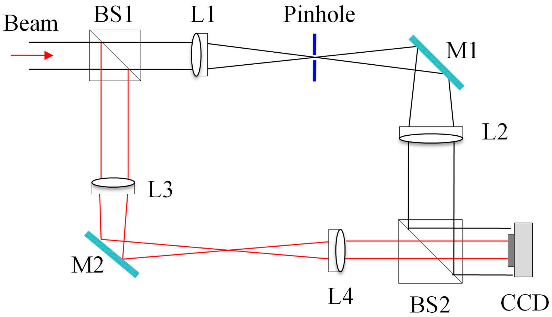
The experimental setup of SRI-WFS, which can be seen as a modified Mach-Zehnder radial shearing interferometer [34,35,36], is shown in Figure 1. This optical system consists of two beam-splitters, BS1 and BS2; a spatial filter, pinhole; two mirrors, M1 and M2; a two-lens positive telescope imaging systems which consisted of two lens, L1 and L2, with focal lengths of f1 = 100 mm and f2 = 300 mm, respectively; and another two-lens positive telescope imaging systems which consisted of two lens, L3 and L4, with focal lengths of f3 = 300 mm and f4 = 100 mm, respectively. A pinhole plate, functioning as a low-pass spatial filter, is placed at the common focal plane of Lens L1 and L2. The signal and reference waves formed interference pattern in the CCD plane. Here we define, g = f2/f1 = f3/f4, and the magnification of SRI-WFS is defined as G = g2. Compared to the tradition radial shearing interferometer configuration, in our experimental setup as shown in Figure 1, we made an improvement by simultaneously using a pinhole filter and a telescope system in each arm of SRI-WFS to generate a promising reference wave.
2.2. Reconstruction of Complex Amplitude Field
For simplicity, we denote the field of the incident test beam as,
where r and ϕ are radial and circular coordinates, respectively; u(r, ϕ) denotes the amplitude and φ(r, ϕ) is the phase information of incident test beam. As shown in Figure 1, the incident beam was split into two beams by the beam-splitter BS1, the reflected beam, and transmitted beam, which acted as signal wave and reference wave, respectively. The reflected beam travels along the invert telescope which consists of lens L3 and L4, and forms a constructed beam and served as a signal wave,
Here, g is the amplification factor of the invert telescope and it is defined as g = f3/f4; R in the reflectivity of BS1. The signal wave contains all the information (including in the amplitude u(gr, ϕ) and the phase φ(gr, ϕ)) of the tested beam E(r, ϕ). The transmitted beam served as a reference wave which can be deduced by Fourier optics theory [37,38,39,40],
where u(r/g, ϕ) represents the amplitude of the reference wave; and (r/g, ϕ) is the wavefront phase of the reference wave; ⊗ is the two-dimensional convolution operator. T(r/g, ϕ) is the Fourier transform of the pinhole with diameter dpin, and it is given by [40],
Here J1 is a first-order Bessel function of the first kind.
The signal wave Es(gr, ϕ) and the reference wave Er(r/g, ϕ) interfere in their superposition area (gr, ϕ). Therefore, the fringe pattern produced by the signal wave Es(gr, ϕ) and the reference wave Er(r/g, ϕ) captured by the CCD can be expressed as,
where κ denotes the linear carrier-frequency coming from an angle between the reference and signal waves, which is formed by slightly tilting beam-splitter BS2.
Considering the contracted signal wave and enlarged reference wave in the SRI-WFS system, we redefine the overlapping area, (rg, ϕ), responding to the field of the signal wave, as a new coordinate domain (r′, ϕ). The field of signal wave can be shown as (r′, ϕ), and the reference wave is shown as E(r′/g2, ϕ). Therefore, the Equation (5) can be rewritten as,
where G = g2 is the magnification of the SRI-WFS. For simplicity, we define the overlapping area (x/G, y/G) as new coordinate domain (x, y) and its intensity distribution in the CCD plane can be written into a general form of the fringe pattern, as follows,
where a(x, y) ∝ Es2(x, y) + Er2(x/G, y/G) is the background intensity, and b(x, y) ∝ 2us(x, y)ur(x/G, y/G) is the modulation intensity of fringe pattern; κx and κy are the carrier-frequency components along x-direction and y-direction, respectively. Therefore, the complex amplitude of modulation (CAM) function [41] of the interferogram as shown in Equation (7) can be easily extracted by spatial phase modulation (SPM) technology, proposed firstly by M. Takeda [33]. The CAM function contains both information of the wavefront phase φ(x, y) and amplitude Es(x, y) of the test beams.
Taking the Fourier transform in two-dimension for the interference pattern [33,42,43],
where FT{ } denotes the Fourier transform, X and Y are the spatial frequency variables, and δ(X, Y) is the Dirac’s delta function, A(X, Y) and B(X, Y) presents the frequency-spectrum of a(x, y) and b(x, y), respectively. The second and third term in Equation (8) are two Dirac’s functions placed in (κx, κy) and (κx, κy) around the low spatial frequency A(X, Y), respectively. By using of a band pass filter, it is possible to extracts the Dirac delta function δ(X − κx, Y − κy). Then, tacking the inverse two-dimension Fourier transform of the Dirac’s delta function δ(X − κx, Y − κy), that is, obtaining the CAM function, as follows [24],
In this equation, it can be seen that it is similar to the description of complex amplitude of the test wave which is expressed in Equation (1). If the magnification G of SRI-WFS is large enough, the term Er(x/G, y/G) will approach to a uniform plane wave, that is, the amplitude tends to ur(0, 0) and the phase component tends to an ideal plane φ(0, 0). Taking into account the amplitude is a relative value in practical application, and the coefficient ur(0, 0) in the Equation (9) can be rewritten as a constant C. Thus, the complex amplitude distribution of test laser beam can be expressed as [24],
3. Determination of M2-Curve
3.1. Measurement Method for Beam Quality Factor M2 Based on the Complex Amplitude Distribution [24]
Once the complex amplitude field E(x, y, 0) of the test laser beam is obtained, according to the diffraction integral theory [37,44], the complete complex amplitude fields E(x, y, z) at z planes after propagation distance z can be calculated using a double fast Fourier transform algorithm [44],
where z is the propagation distance, k is wave number, λ is wavelength of test laser beam, ηx = x/λz, ηy = y/λz are the spatial frequencies, respectively. The direct (FT) and inverse (FT−1) Fourier transform are calculated using a Fast Fourier Transform algorithm. Furthermore, in accordance with the ISO standard [4,5,6], the complex amplitude fields E(x, y, z) can be used to determine the beam parameters relevant for beam propagation, i.e., beam widths wx(z) and wy(z). Performing a hyperbolic fit to the beam width along the beam transmission axis,
where wx,y is the beam width in the x-direction or y-direction; ax,y, bx,y and cx,y are the hyperbolic fitting coefficients, and the subscript x and y correspond to the values along the x-direction or y-direction, respectively. Then the waist radius wx0,y0, divergence half angle θx,y and beam propagation factor can be calculated from the following expressions [4],
According to above analysis (Section 2.1, Section 2.2 and Section 3.1), as long as the phase φ(x, y) and the amplitude u(x, y) of the test laser beam are obtained, it is possible to calculate the beam quality M2 factor, specifically, the values of and along x-direction and y-direction of the test beams, respectively.
3.2. M2-Curve
The output beam of a multimode-laser stable cavity with rectangular geometry in many transverse modes can be written as an incoherent superposition of Hermite-Gaussian (HG) beams [45,46]. Usually the spatial modes are separable; the complex amplitude field distribution of HG modes, at the plane z = 0, can be written as [45],
where the phase term is ignored, is the waist radius of the fundamental mode HG00; and Hm and Hn denotes the Hermite-polynomial of order m in x-direction and order n in y-direction, respectively. HG modes are one set of orthogonal eigenfunctions of the scalar Helmholtz wave equation. Due to the completeness of this eigenfunction set, an arbitrary transverse wave field E(x, y, z) can be expanded into a superposition of HG modes [46],
with
where the asterisk denotes complex conjugation operator; cmn is the complex-valued expansion coefficients, cmn = Cmnexp(φmn), including in the modal amplitude Cmn = |cmn| and phase φmn = angle(cmn).
As the analysis above, generally, the intensity profile of the output beam emitted by a multimode stable cavity is non-rotational symmetric or asymmetric beams, as shown in Figure 2. According to Sigman’s theories [1,2], the quality of the laser beam is evaluated by in x-direction and in y-direction. However, we found that the values of and are non-unique if we rotate coordinate the axis in an astigmatic laser beam. Consequently, just using the simple parameters and to characterize the beam quality of an asymmetric beam is not comprehensive or objective [9,29,30].
Similarly to the traditional definitions form of the beam widths in the general astigmatic beam [4], we have
and
and
and
where and are the centroid coordinates of the power density distribution which defined as the first-order moment of the power density distribution of the test beams. Therefore, the corresponding beam divergence half angles are given by [4],
Therefore, the beam widths and the beam divergence half angles of the original and rotated beam (with a rotation angle α) have the following relationships which are given by the Equations (28)–(31), respectively; as following [30,32],
Utilizing the Equations (28)–(31), it is easy to derive the following expressions,
In this case, we can derive a new beam propagation ratio M2(α) with rotation angle α to characterize the rotated beam and it can be given as,
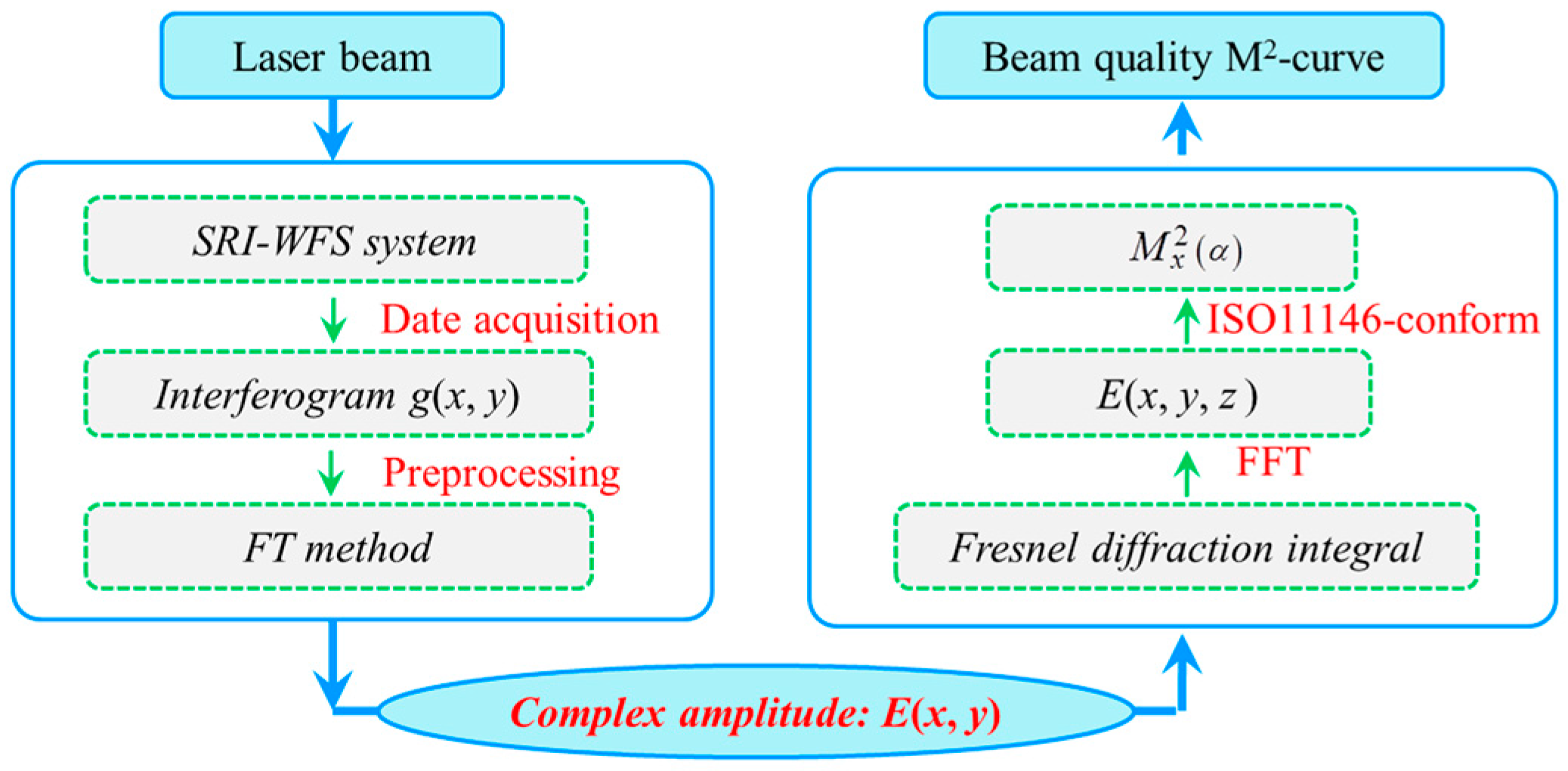
where and are waist radius and divergence half angle in the x-direction with a rotation angle α of coordinate axis, respectively. M2 can obtain different values if the rotation angle α charges with the coordinate axis, that is, a track of the M2 values versus the rotation angle (α) of the beam coordinate axis will be form and named M2-curve which is unique to a specific tested beam. It can be seen from the Equation (35) that the M2-curve takes into account changes in angle and can give a track of the M2 values which is compared to the rotation angle α of the beam coordinate axis. That is, the M2-curve contains all the values of beam quality M2 in all directions. The traditional M2 factor in x-direction and in y-direction are just special cases of the M2-curve in a special direction of the tested beam, precisely in two orthogonal directions (x-axis and y-axis). Therefore, the M2-curve has a more comprehensive physical meaning and is more objective for characterizing the beam quality because it can be uniquely determined for a particular tested beam. In other words, there is a one-to-one mapping relationship between a particular tested beam and its sharp of M2-curve. According to the above analysis in Section 2 and Section 3, we can summarize the flow chart of the M2-curve determined by the SRI-WFS method, as shown in Figure 3.
4. Experiment Results and Discussions
The beams from a diode pump solid state laser (DPSSL) with 532 nm wavelength are used as test beam. The excitation of mode mixture in the DPSSL are Hermite-Gaussian-like modes (shorted as TELMmn) is achieved by adjusting the tilt angle of the cavity mirrors [45]. The experiment setup of SRI-WFS for completely reconstructing the complex amplitude field of a laser beam is depicted in Figure 1, and it has been demonstrated that it can be used for beam quality measurements in real-time and the details of SRI-WFS system can be seen in [24]. Two invert telescopes with telescope factor g = 3, consisted of achromatic lens L1–L4 with focal length f1 = f4 = 100 mm and f2 = f3 = 300 mm, respecting the magnification G = 9 of SRI-WFS. A pinhole plate with diameter dpin = 25 μm is used to generate a reference wave. A CCD camera, model MVIC-II-1MM, with 1024 × 1280 pixels and 5.2 micron in each pixel, is positioned at the imaging plane to record interferogram in real time. The CCD sampled-data are sent to the personal computer system (PC) for further processing.
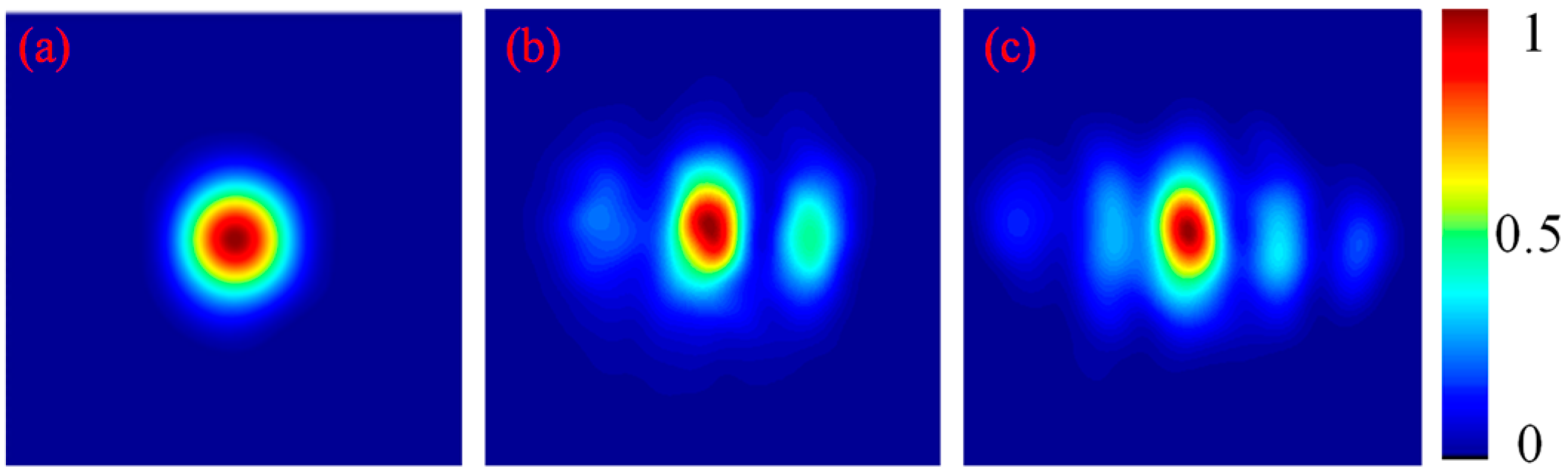
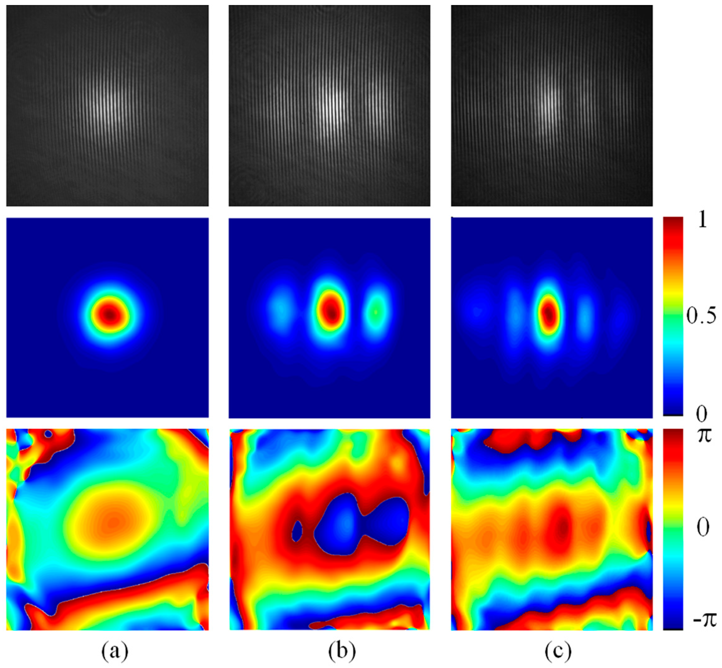
Adjusting a slight tilt angle in the cavity mirrors, we can obtain different mix-mode beam outputs whose intensity profiles are similar to the Hermite-Gaussian mode in TEMmn. For the convenience of the following analysis, we denote these mix-mode beams as Hermite-Gaussian-like modes in TELMmn to distinguish with the pure Hermite-Gaussian modes in TEMmn. As shown in Figure 4, three intensity profiles corresponding to Hermite-Gaussian-like modes in TELM00, TELM20, and TELM40, respectively, are used as the test beams in our experiments. Corresponding interferograms formed with SRI-WFS are shown in Figure 5 (up row). The reconstructed intensity profiles (middle row) and the reconstructed wrapped phase distribution (low row) of the test beams are also shown in Figure 5. Each reconstructed distributions of amplitude and phase for the test beams are extracted from a single interferogram according to Equations (7)–(10). Considering the limited of conditions in our laboratory, we only investigate the intensity distribution for comparative analysis. For a quantitative comparison of the measurement and reconstruction intensity profile, two-dimension cross-correlation coefficient Cc is used as a metric [24]. Here Cc is defined as the cross-correlation between the images of measurement intensity distribution IM(x, y) and reconstruction intensity distribution IR(x, y), and Cc = 1 is indicated that the measured intensity profile and reconstructed intensity profiles match perfectly. In our experiment, the Cc of the reconstructed and measurement intensities for the Hermite-Gaussian-like modes in TELM00, TELM20 and TELM40 are 0.999, 0.998 and 0.997, respectively.
There are several causes for the deviation of the reconstruction intensity and the measured intensity: (1) optical components such as inaccurate errors of telescope system and misalignment in the SRI-WFS system lead to beam distortion; (2) the intensity of the reference wave hardly becomes completely flat with the limited magnification of SRI-WFS in practice; (3) filtering error in the Fourier transform method for interferogram analysis; etc. As long as reconstructing the complex amplitude field E(x, y, 0) of the test beams, the field E(x, y, z) at different plane of z-axis direction (with different propagation length z) can be determined easily according to the Equation (11), and the intensities distribution I(x, y, z) = |E(x, y, z)|2 are also determined uniquely. According to the Standard ISO11146, the beam width wxz can be determined by the second moment of the obtained intensity distributions, as described in Equations (19)–(22). The beam width wxz of test beams in x-direction of Hermite-Gaussian-like modes TELM00, TELM20, and TELM40 can be calculated directly from the intensity distribution I(x, y, z) at different propagation location z. Moreover, according to the Equations (13) and (28)–(31), the beam widths wxzα and the beam divergence half angles θxzα with different rotation angle α of the coordinate axis also can be obtained. Figure 6 shows the results of the beam width wxzα in the x-direction of Hermite-Gaussian-like modes (a) TELM00; (b) TELM20 and (c) TELM40 versus propagation distance z and the different rotation angle α of coordinate axis. Here, the rotation angles α are settled to 10, 20, 30, 40, 50, 60, 70, 80 and 90°; respectively.
It can be seen from Figure 6 that with the different rotation angle α, for example, α= 10, 20, 30, 40, 50, 60, 70, 80, and 90°; the beam widths wx, the beam waist radius wx0, beam divergence half angles θx, and waist positions z0 of the tested beams are all very different. It is further evidenced by the results of the normalized waist radius wxα(z0) and beam divergence half angles θx in the x-directions for Hermite-Gaussian-like modes (TELM00, TELM20, and TELM40) versus rotation angle of coordinate axis α, as shown in Figure 7. That is, with the changing rotation angle of the coordinate axis of the tested beam in actual measurement, the waist radius wx0 and divergence half angle θx are ever-changes and these different will directly result in the non-unique of the values of M2 factor. Obviously, it is consistent with the previous analysis and the motivation of this paper. Moreover, it also indicates that using the simple M2 factor, in x-direction and in y-direction just two special cases (in the two orthogonal directions) of the test beams but missing the most of information in the other random rotation angles α of the test beams.
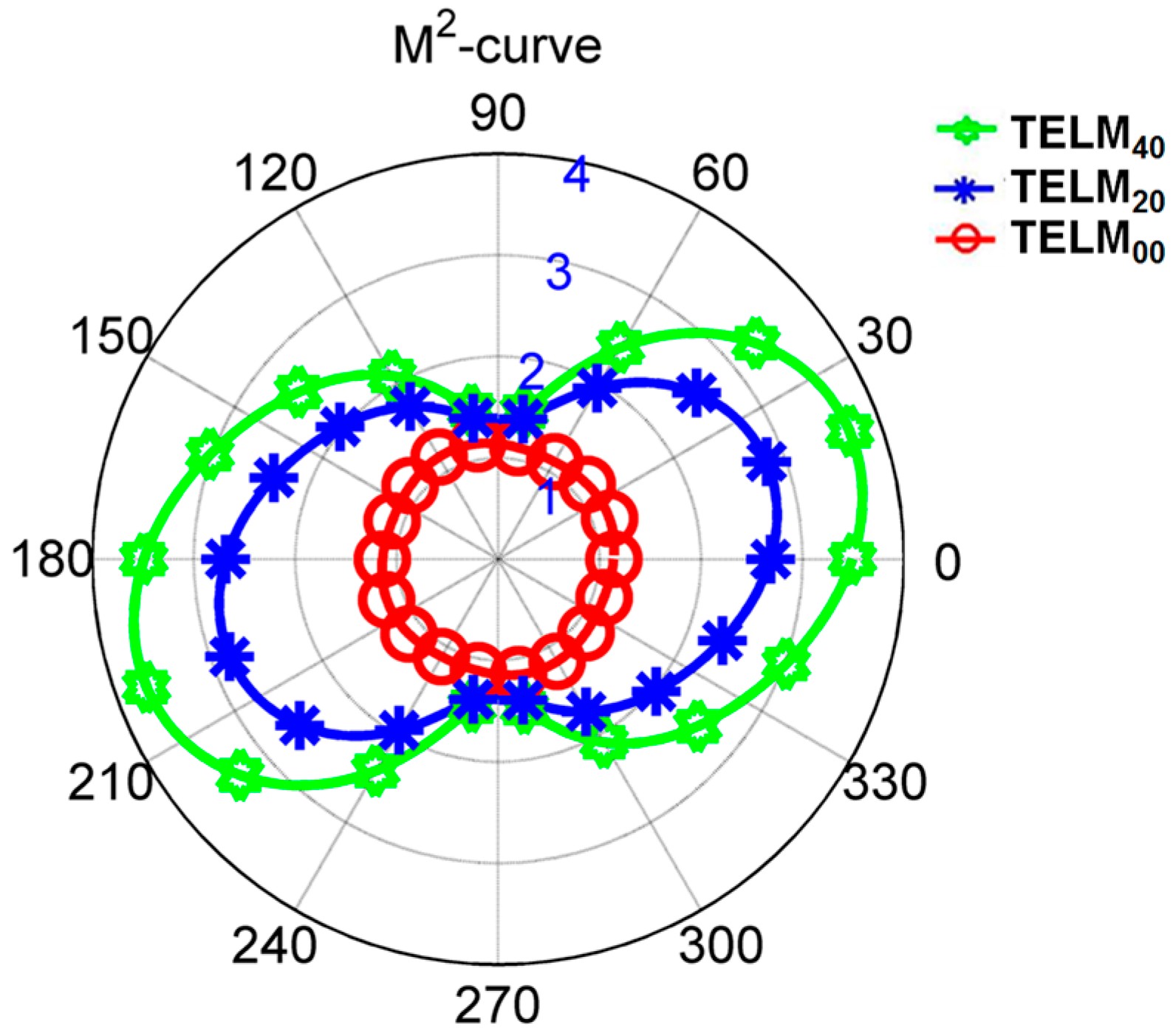
The results of the M2-curves of the test beams (Hermite-Gaussian-like modes TELM00, TELM20, and TELM40) are shown in Figure 8. Note that all the M2-curves for Hermite-Gaussian-like modes TELM00, TELM20, and TELM40 are asymmetric. The M2-curve is maybe a circle, an ellipse, or an 8-shaped pattern. Moreover, the length values, from the original point to the cross-point at the curve, denote the M2 values along this rotation angle α. For example, as shown in Figure 8, the values of the test beams, Hermite-Gaussian-like modes TELM00, TELM20 and TELM40 along α = 0 direction, which corresponding to the traditional M2 factor along x-direction of the tested beams, are 1.06, 2.62 and 3.72, respectively. Moreover, when the rotation angle α is equal to 90°, corresponding to along the y-direction for the tradition M2 factor. In this case, the values of are 1.08 for TELM00, 1.27 for TELM20, and 1.37 for TELM40, respectively. For comparative analysis, we also measured the beam propagation factor M2 values using the traditional ISO11146 standard based beam quality analyzer (BQA) developed in our previous work [25], and the results are shown in Table 1. It shows that the beam quality M2 factors with ISO11146 standard based method are = 1.04, = 2.54 and = 3.56 along the x-direction and = 1.06, = 1.20 and = 1.32 along the y-direction for Hermite-Gaussian-like modes TELM00, TELM20, and TELM40, respectively. Table 1 also shows the measurement errors between the M2 factor values of Hermite-Gaussian-like modes TELM00, TELM20, and TELM40 with the proposed SRI-WFS method and the ISO1116 standard based BQA. The maximum measured deviation of the two methods are 4.49% for and 5.83% for along x-axis and y-axis, respectively. It can be seen from Table 1 that the results of both measurement methods are well in agreement.
As shown in Figure 8, the M2-curve include in all M2 information (including in the traditional M2 factor values) in all random rotation angle α of the coordinate axis. From this sense, M2-curve is an extension method for characterization of beam quality. Moreover, its shape will be uniquely determined for a particular test beam. Consequently, it provides a more comprehensive and more objective physical meaning for actual applications.
5. Conclusions
The non-uniqueness of characterization of laser beam quality with the traditional M2 factor can be overcome by using the M2-curve. The M2-curve has more general physical meaning and wider application scope both for asymmetric beams and astigmatic beams. The M2-curve not only contains the beam quality terms, and , to evaluate the beam propagation quality in the x-direction and y-direction, respectively; but also introduces a curve of which is used to characterize beam propagation factor versus the rotation angle α of coordinate axis. Moreover, the measurement method of the M2-curve based on modified SRI-WFS is also put forward which is used to demonstrate the potential of the proposed method, M2-curve, for charactering asymmetric beams.
Acknowledgments
This work is supported by the grants from National Natural Science Foundation of China (No. 61605048), Natural Science Foundation of Fujian Province, China (No. 2016J01300), Fujian Scientific Research Platform for Innovation, China, (No. 2013H2002), and the Scientific Research Funds of Huaqiao University (No. 15BS413). Yongzhao Du thanks Guoying Feng (Sichuan University, China) for supporting this work and providing helpful discussion, and Max Wiedmann for improving the writing and expression in the manuscript.
Author Contributions
Yongzhao Du conceived and designed the experiments, performed the experiments, analyzed the data and wrote the paper.
Conflicts of Interest
The authors declare no conflict of interest.
References
- Siegman, A.E. New developments in laser resonators, in Optical Resonators. Proc. SPIE 1990, 1224, 2–14. [Google Scholar]
- Siegman, A.E. Defining, measuring, and optimizing laser beam quality. Proc. SPIE 1993, 1868, 2–13. [Google Scholar]
- International Standardization for Standardization. Terminology and Test Methods ISO/TC172/SC/WG1; ISO: Geneva, Switzerland, 1991. [Google Scholar]
- International Standardization for Standardization. ISO 11146-1 Lasers and Laser-Related Equipment—Test Methods for Laser Beam Widths, Divergence Angles and Beam Propagation Ratios—Part 1: Stigmatic and Simple Astigmatic Beams; ISO: Geneva, Switzerland, 2005. [Google Scholar]
- International Standardization for Standardization. ISO 11146-2, Lasers and Laser-Related Equipment—Test Methods for Laser Beam Widths, Divergence Angles and Beam Propagation Ratios—Part 2: General Astigmatic Beams; ISO: Geneva, Switzerland, 2005. [Google Scholar]
- International Standardization for Standardization. ISO 11146-3, Lasers and Laser-Related Equipment—Test Methods for Laser Beam Widths, Divergence Angles and Beam Propagation Ratios—Part 3: Intrinsic and Geometrical Laser Beam Classification, Propagation and Details of Test Methods; ISO: Geneva, Switzerland, 2004. [Google Scholar]
- Bouafia, M.; Bencheikh, H.; Bouamama, L.; Weber, H. M2 quality factor as a key to mastering laser beam propagation. Proc. SPIE 2004, 5456, 130–140. [Google Scholar]
- Paschotta, R. Beam quality deterioration of lasers caused by intracavity beam distortions. Opt. Express 2006, 14, 6069–6074. [Google Scholar] [CrossRef] [PubMed]
- Feng, G.-Y.; Zhou, S. Discussion of comprehensive evaluation on laser beam quality. Chin. J. Laser 2009, 36, 1643–1653. [Google Scholar]
- Newburgh, G.A.; Michael, A.; Dubinskii, M. Composite Yb:YAG/SiC-prism thin disk laser. Opt. Express 2010, 18, 17066–17074. [Google Scholar] [CrossRef] [PubMed]
- Borgentun, C.; Bengtsson, J.; Larsson, A. Full characterization of a high-power semiconductor disk laser beam with simultaneous capture of optimally sized focus and far-field. Appl. Opt. 2011, 50, 1640–1649. [Google Scholar] [CrossRef] [PubMed]
- Xiang, Z.; Wang, D.; Pan, S.; Dong, Y.; Zhao, Z.; Li, T.; Ge, J.; Liu, C.; Chen, J. Beam quality improvement by gain guiding effect in end-pumped Nd:YVO4 laser amplifiers. Opt. Express 2011, 19, 21060–21073. [Google Scholar] [CrossRef] [PubMed]
- Scaggs, M.; Haas, G. Real time monitoring of thermal lensing of a multikilowatt fiber laser optical system. In Proceedings of the Laser Resonators, Microresonators, and Beam Control XIV, San Francisco, CA, USA, 22–25 January 2012.
- Gong, M.L.; Qiu, Y.; Huang, L.; Liu, Q.; Yan, P.; Zhang, H.T. Beam quality improvement by joint compensation of amplitude and phase. Opt. Lett. 2013, 38, 1101–1103. [Google Scholar] [CrossRef] [PubMed]
- Schäfer, B.; Mann, K. Determination of beam parameters and coherence properties of laser radiation by use of an extended Hartmann-Shack wave-front sensor. Appl. Opt. 2002, 41, 2809–2817. [Google Scholar] [CrossRef] [PubMed]
- Schäfer, B.; Lübbecke, M.; Mann, K. Hartmann-Shack wave front measurements for real time determination of laser beam propagation parameters. Rev. Sci. Instrum. 2006, 77, 053103. [Google Scholar] [CrossRef]
- Neubert, B.J.; Huber, G.; Scharfe, W. On the problem of M2 analysis using Shack-Hartmann measurements. J. Phys. D Appl. Phys. 2001, 34, 2414–2419. [Google Scholar] [CrossRef]
- Sheldakova, J.V.; Kudryashov, A.V.; Zavalova, V.Y.; Cherezova, T.Y. Beam quality measurements with Shack-Hartmann wavefront sensor and M2-sensor: Comparison of two methods. In Proceedings of the Laser Resonators and Beam Control IX, San Jose, CA, USA, 22–24 January 2007.
- Lambert, R.W.; Cortés-Martínez, R.; Waddle, A.J.; Shephard, J.D.; Taghizadeh, M.R.; Greenaway, A.H.; Hand, D.P. Compact optical system for pulse-to-pulse laser beam quality measurement and applications in laser machining. Appl. Opt. 2004, 43, 5037–5046. [Google Scholar] [CrossRef] [PubMed]
- Schmidt, O.A.; Schulze, C.; Flamm, D.; Brüning, R.; Kaiser, T.; Schröoter, S.; Duparré, M. Real-time determination of laser beam quality by modal decomposition. Opt. Express 2011, 19, 6741–6748. [Google Scholar] [CrossRef] [PubMed]
- Flamm, D.; Schulze, C.; Brüning, R.; Schmidt, O.A.; Kaiser, T.; Schröter, S.; Duparré, M. Fast M2 measurement for fiber beams based on modal analysis. Appl. Opt. 2012, 51, 987–996. [Google Scholar] [CrossRef] [PubMed]
- Schulze, C.; Flamm, D.; Duparré, M.; Forbes, A. Beam-quality measurements using a spatial light modulator. Opt. Lett. 2012, 37, 4867–4869. [Google Scholar] [CrossRef]
- Offerhaus, H.L.; Edwards, C.B.; Witteman, W.J. Single shot beam quality (M2) measurement using a spatial Fourier transform of the near field. Opt. Commun. 1998, 151, 65–68. [Google Scholar] [CrossRef]
- Du, Y.-Z.; Feng, G.-Y.; Li, H.; Cai, Z.; Zhao, H.; Zhou, S. Real-time determination of beam propagation factor by Mach-Zehnder point diffraction interferometer. Opt. Commun. 2013, 287, 1–5. [Google Scholar] [CrossRef]
- Feldman, M.; Mockler, D.J.; English, R.E.; Byrd, J.L., Jr.; Salmon, J.T. Self-referencing Mach-Zehnder interferometer as a laser system diagnostic. In Proceedings of the Active and Adaptive Optical Systems, San Diego, CA, USA, 22–24 July 1991.
- Rhoadarmer, T.A. Development of a self-referencing interferometer wavefront sensor. Proc. SPIE Adv. Wavefront Control Methods Devices Appl. II 2004, 5553, 112–126. [Google Scholar]
- Nemes, G.; Siegman, A.E. Measurement of all ten second-order moments of an astigmatic beam by the use of rotating simple astigmatic (anamorphic) optics. J. Opt. Soc. Am. A 1994, 11, 2257–2263. [Google Scholar] [CrossRef]
- Kochkina, E.; Wanner, G.; Schmelzer, D.; Tröbs, M.; Heinzel, G. Modeling of the general astigmatic Gaussian beam and its propagation through 3D optical systems. Appl. Opt. 2013, 52, 6030–6040. [Google Scholar] [CrossRef] [PubMed]
- Deng, G.; Feng, G.; Li, W.; Zhang, T.; Liao, H.; Zhou, S. Experimental study of beam quality factor M2 matrix for non-circular symmetry beam. Chin. J. Laser 2009, 36, 2014–2018. [Google Scholar] [CrossRef]
- Li, W.; Feng, G.; Huang, Y.; Deng, G.; Huang, Y.; Chen, J.; Zhou, S. Matrix formulation of the beam quality of the Hermite-Gaussian beam. Laser Phys. 2009, 19, 1–6. [Google Scholar] [CrossRef]
- Li, W.; Feng, G.-Y.; Huang, Y.; Li, G.; Yang, H.-M.; Xie, X.-D.; Chen, J.-G.; Zhou, S.-H. M2 factor matrix for two-dimensional Hermite-Gaussian beam. Acta Phys. Sin. 2009, 58, 2461–2466. [Google Scholar]
- Liu, X.-L.; Feng, G.-Y.; Li, W.; Tang, C.; Zhou, S.-H. Theoretical and experimental study on M2 factor matrix for astigmatic elliptical Gaussian beam. Acta Phys. Sin. 2013, 62, 194202. [Google Scholar]
- Takeda, M.; Ina, H.; Kobayashi, S. Fourier transform method of fringe pattern analysis for computer-based topography and interferometry. J. Opt. Soc. Am. 1982, 72, 156–160. [Google Scholar] [CrossRef]
- Kohler, D.R.; Gamiz, V.L. Interferogram reduction for radial-shear and local-reference-holographic interferograms. App. Opt. 1986, 25, 1650–1652. [Google Scholar] [CrossRef]
- Notaras, J.; Paterson, C. Demonstration of closed-loop adaptive optics with a point-diffraction interferometer in strong scintillation with optical vortices. Opt. Express 2007, 15, 13745–13756. [Google Scholar]
- Notaras, J.; Paterson, C. Point-diffraction interferometer for atmospheric adaptive optics in strong scintillation. Opt. Commun. 2008, 281, 360–367. [Google Scholar] [CrossRef]
- Goodman, J.W. Introduction to Fourier Optics, 2nd ed.; McGraw-Hill: New York, NY, USA, 1968; pp. 63–90. [Google Scholar]
- Smartt, R.N.; Stell, W.H. Theory and Application of Point-Diffraction Interferometers. Jpn. J. Appl. Phys. 1975, 14, 351–356. [Google Scholar] [CrossRef]
- Koliopoulos, C.; Kwon, O.; Shagam, R.; Wyant, J.C.; Hayslett, C.R. Infrared point-diffraction interferometer. Opt. Lett. 1978, 3, 118–120. [Google Scholar] [CrossRef] [PubMed]
- Mercer, C.R.; Creath, K. Liquid-crystal point-diffraction interferometer for wave-front measurement. Appl. Opt. 1996, 35, 1633–1642. [Google Scholar] [CrossRef] [PubMed]
- Lago, E.L.; dela Fuente, R. Amplitude and phase reconstruction by radial shearing interferometry. Appl. Opt. 2008, 47, 372–377. [Google Scholar] [CrossRef]
- Bone, D.J.; Bachor, H.-A.; Sandeman, R.J. Fringe-pattern analysis using a 2-D Fourier transform. Appl. Opt. 1986, 25, 1653–1660. [Google Scholar] [CrossRef] [PubMed]
- Roddier, C.; Roddier, F. Interferogram analysis using Fourier transform techniques. Appl. Opt. 1987, 26, 1668–1673. [Google Scholar] [CrossRef] [PubMed]
- Mendlovic, D.; Zalevsky, Z.; Konforti, N. Computation considefactorns and fast algorithms for calculating the diffraction integral. J. Mod. Opt. 1997, 44, 407–414. [Google Scholar] [CrossRef]
- Kogelnik, H.; Li, T. Laser beams and resonators. Appl. Opt. 1996, 5, 1550–1567. [Google Scholar] [CrossRef] [PubMed]
- Siegman, A.E. Lasers; University Science Books: Mill Valley, CA, USA, 1986; pp. 777–811. [Google Scholar]
Figure 1.
Experimental setup of SRI-WFS: BS1, BS2, beam-splitters, L1–L4, lens with the focal length f1 = f4 = 100 mm and f2 = f3 = 300 mm, respectively; pinhole, spatial filtering plate with diameter dpin = 25 μm; M1, M2, reflection mirrors.
Figure 1.
Experimental setup of SRI-WFS: BS1, BS2, beam-splitters, L1–L4, lens with the focal length f1 = f4 = 100 mm and f2 = f3 = 300 mm, respectively; pinhole, spatial filtering plate with diameter dpin = 25 μm; M1, M2, reflection mirrors.

Figure 2.
Asymmetric beam intensity distribution in the laboratory coordinate system.
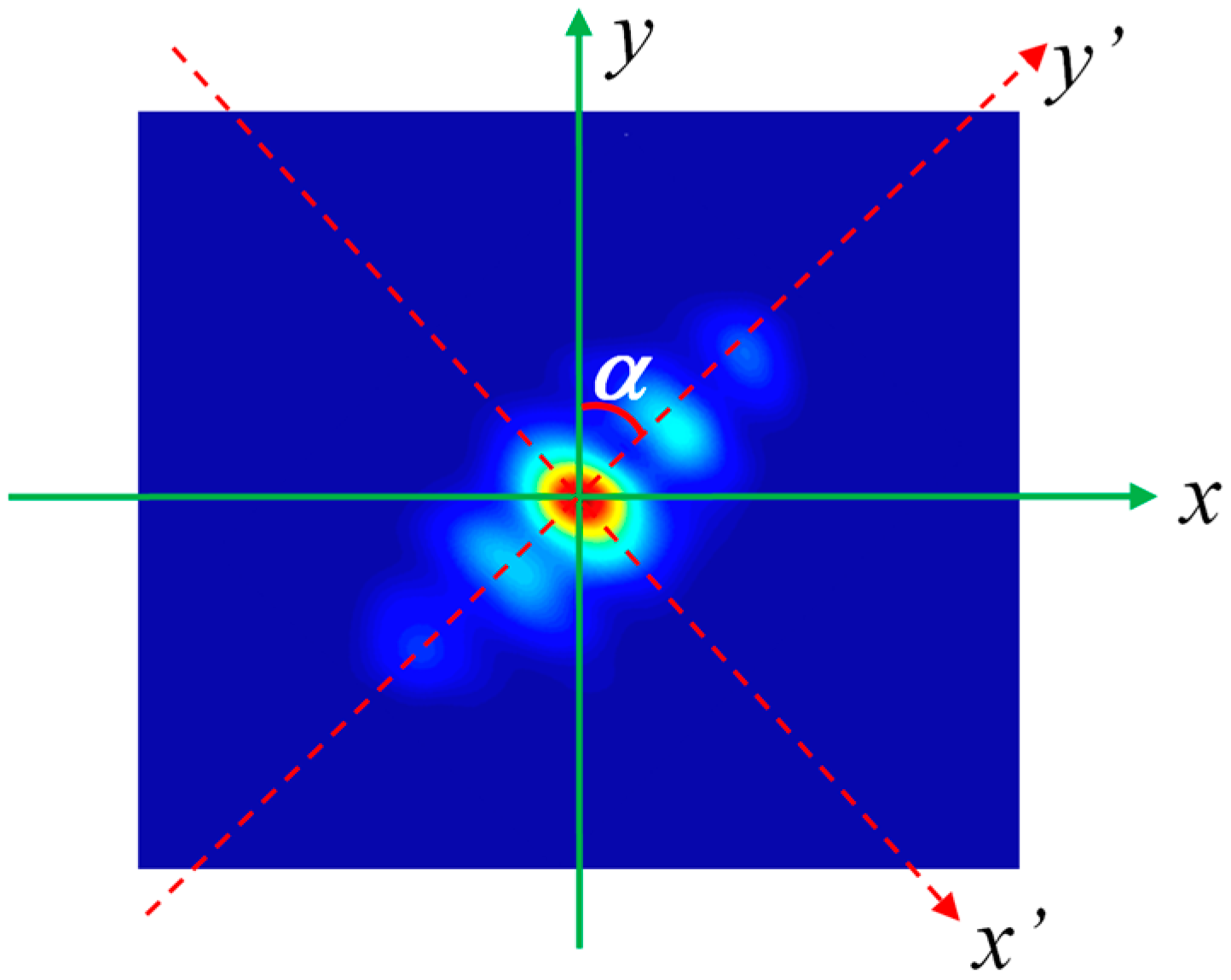
Figure 3.
The flow chart of beam quality M2-curve determined by the proposed SRI-WFS method.

Figure 4.
Measured intensity profiles of Hermite-Gaussian-like modes in (a) TELM00; (b) TELM20 and (c) TELM40.
Figure 4.
Measured intensity profiles of Hermite-Gaussian-like modes in (a) TELM00; (b) TELM20 and (c) TELM40.

Figure 5.
The captured interferogram, reconstructed intensity (a.u.), and wrapped phase maps of Hermite-Gaussian-like modes in (a) TELM00; (b) TELM20 and (c) TELM40. Interferogram (up row), reconstructed intensity profile (middle row), and the reconstructed phase (low row) of the test beams.
Figure 5.
The captured interferogram, reconstructed intensity (a.u.), and wrapped phase maps of Hermite-Gaussian-like modes in (a) TELM00; (b) TELM20 and (c) TELM40. Interferogram (up row), reconstructed intensity profile (middle row), and the reconstructed phase (low row) of the test beams.

Figure 6.
The beam widths wx in x-direction of Hermite-Gaussian-like modes (a) TELM00; (b) TELM20; and (c) TELM40 versus propagation distance. The rotation angle α of the coordinate axis is 10, 20, 30, 40, 50, 60, 70, 80, 90°, respectively.
Figure 6.
The beam widths wx in x-direction of Hermite-Gaussian-like modes (a) TELM00; (b) TELM20; and (c) TELM40 versus propagation distance. The rotation angle α of the coordinate axis is 10, 20, 30, 40, 50, 60, 70, 80, 90°, respectively.
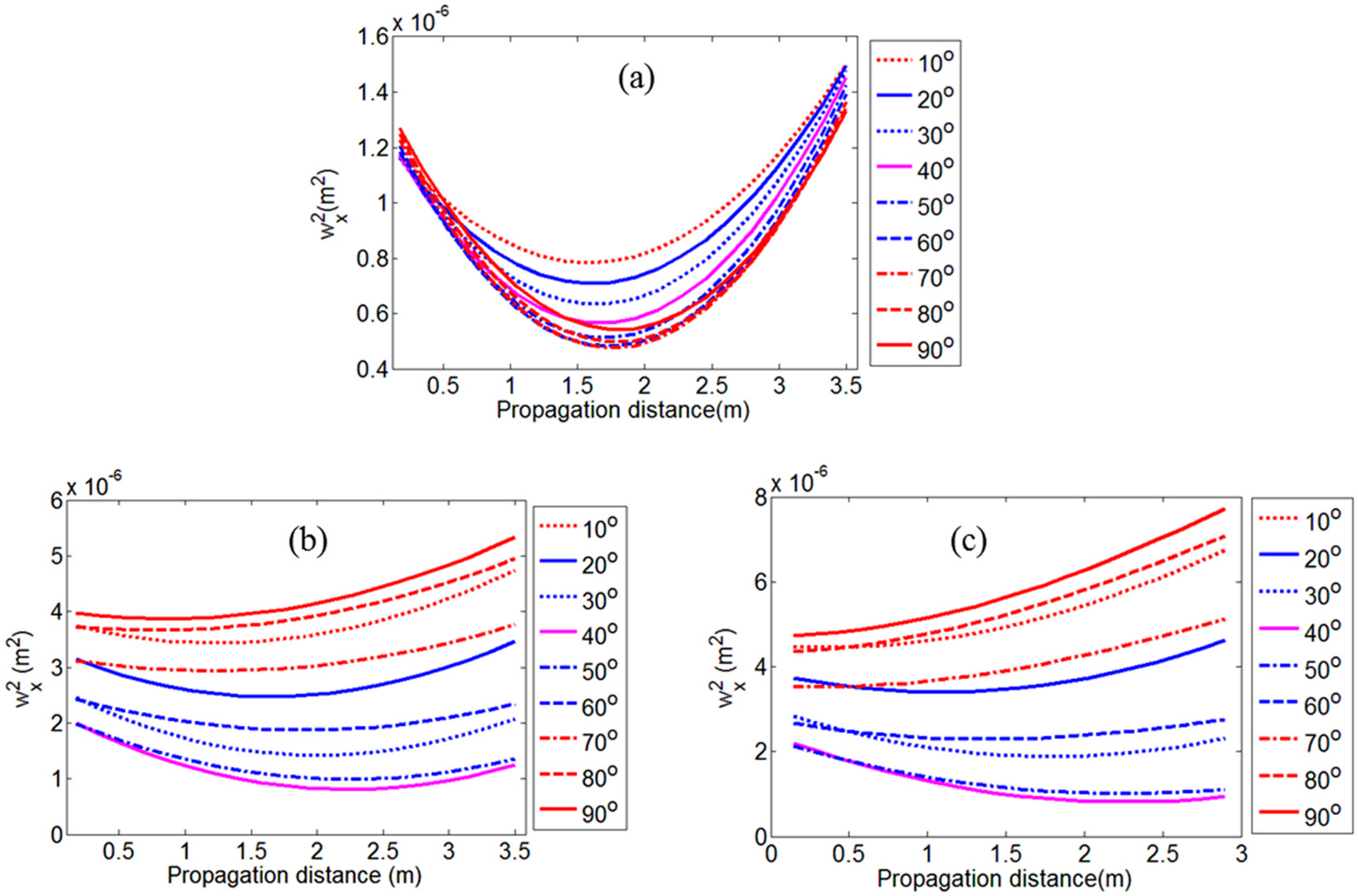
Figure 7.
Normalized waist radius wx0 and divergence half angle θx in x-directions for Hermite-Gaussian-like modes (TELM00, TELM20, and TELM40) versus rotation angle of coordinate axis.
Figure 7.
Normalized waist radius wx0 and divergence half angle θx in x-directions for Hermite-Gaussian-like modes (TELM00, TELM20, and TELM40) versus rotation angle of coordinate axis.
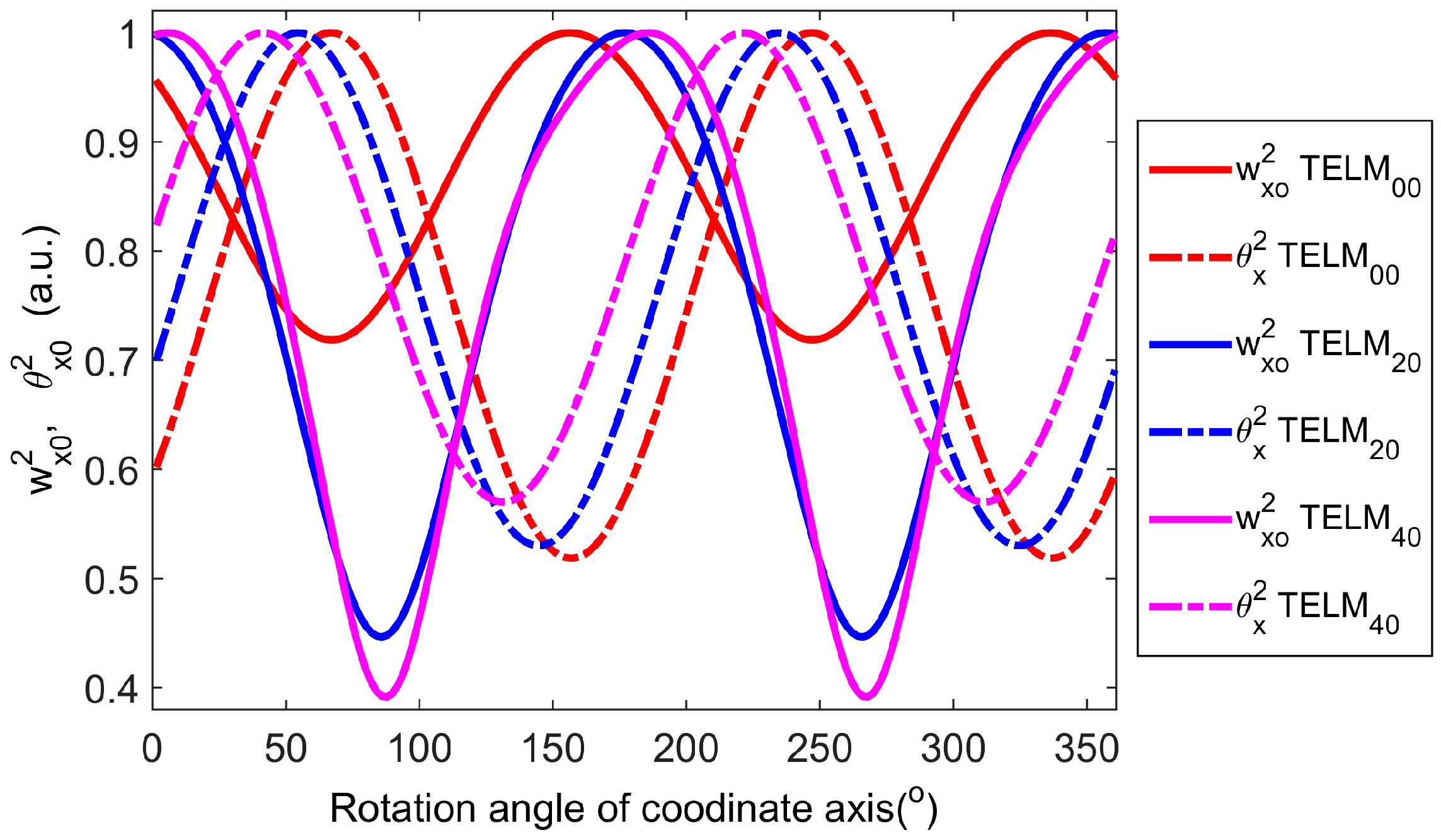
Figure 8.
M2-curves of Hermite-Gaussian-like modes in TELM00, TELM20, and TELM40. Here, the numbers 1, 2, 3, and 4 are the circular scale for the M2-curve.
Figure 8.
M2-curves of Hermite-Gaussian-like modes in TELM00, TELM20, and TELM40. Here, the numbers 1, 2, 3, and 4 are the circular scale for the M2-curve.


Table 1.
The measurement results of M2 factor for Hermite-Gaussian-like modes TELM00, TELM20, and TELM40 with the proposed SRI-WFS method and the ISO1116 standard based beam quality analyzer.
| Beam Quality | ||||||
|---|---|---|---|---|---|---|
| TELM00 | TELM20 | TELM40 | TELM00 | TELM20 | TELM40 | |
| SRI-WFS | 1.06 | 2.62 | 3.72 | 1.08 | 1.27 | 1.37 |
| ISO1116 method | 1.04 | 2.54 | 3.56 | 1.06 | 1.20 | 1.32 |
| Errors (%) | 1.96% | 3.15% | 4.49% | 1.89% | 5.83% | 3.79% |
© 2016 by the author; licensee MDPI, Basel, Switzerland. This article is an open access article distributed under the terms and conditions of the Creative Commons Attribution (CC-BY) license (http://creativecommons.org/licenses/by/4.0/).
Share and Cite
MDPI and ACS Style
Du, Y. Measurement of M2-Curve for Asymmetric Beams by Self-Referencing Interferometer Wavefront Sensor. Sensors 2016, 16, 2014. https://doi.org/10.3390/s16122014
AMA Style
Du Y. Measurement of M2-Curve for Asymmetric Beams by Self-Referencing Interferometer Wavefront Sensor. Sensors. 2016; 16(12):2014. https://doi.org/10.3390/s16122014
Chicago/Turabian StyleDu, Yongzhao. 2016. "Measurement of M2-Curve for Asymmetric Beams by Self-Referencing Interferometer Wavefront Sensor" Sensors 16, no. 12: 2014. https://doi.org/10.3390/s16122014
Note that from the first issue of 2016, this journal uses article numbers instead of page numbers. See further details here.