
Mitigating RF Front-End Nonlinearity of Sensor Nodes to Enhance Spectrum Sensing

Abstract
:1. Introduction
2. System Model and Problem Analysis
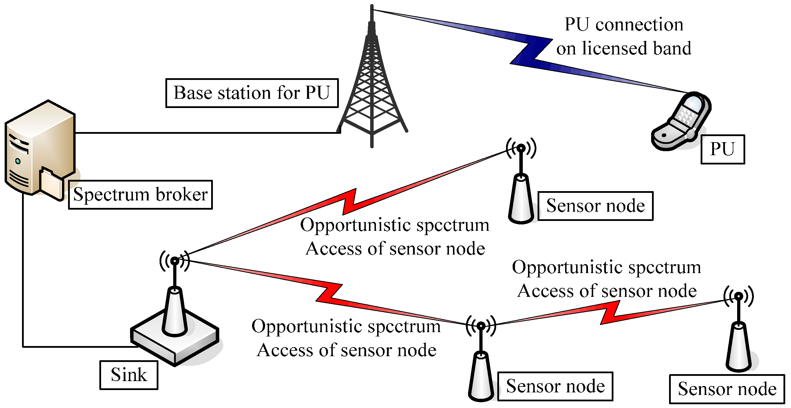
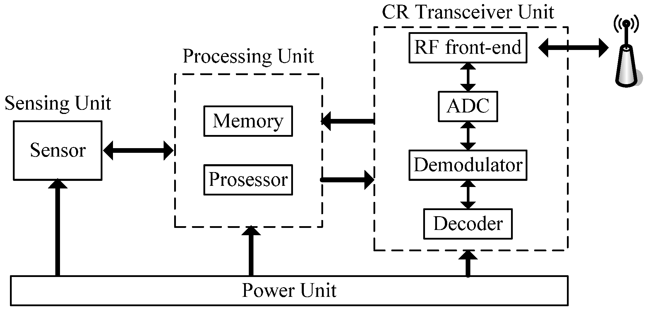
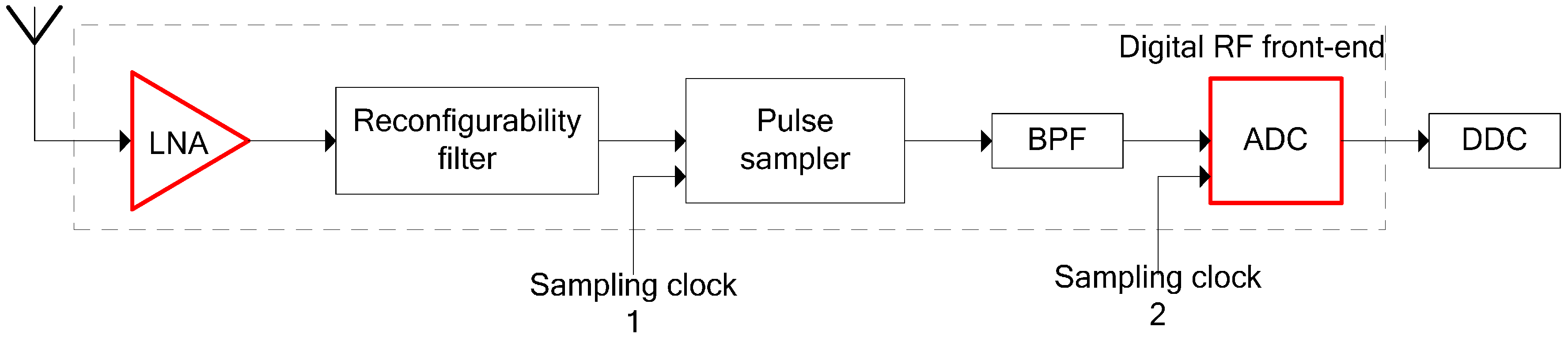
2.1. CR-WSN Architecture
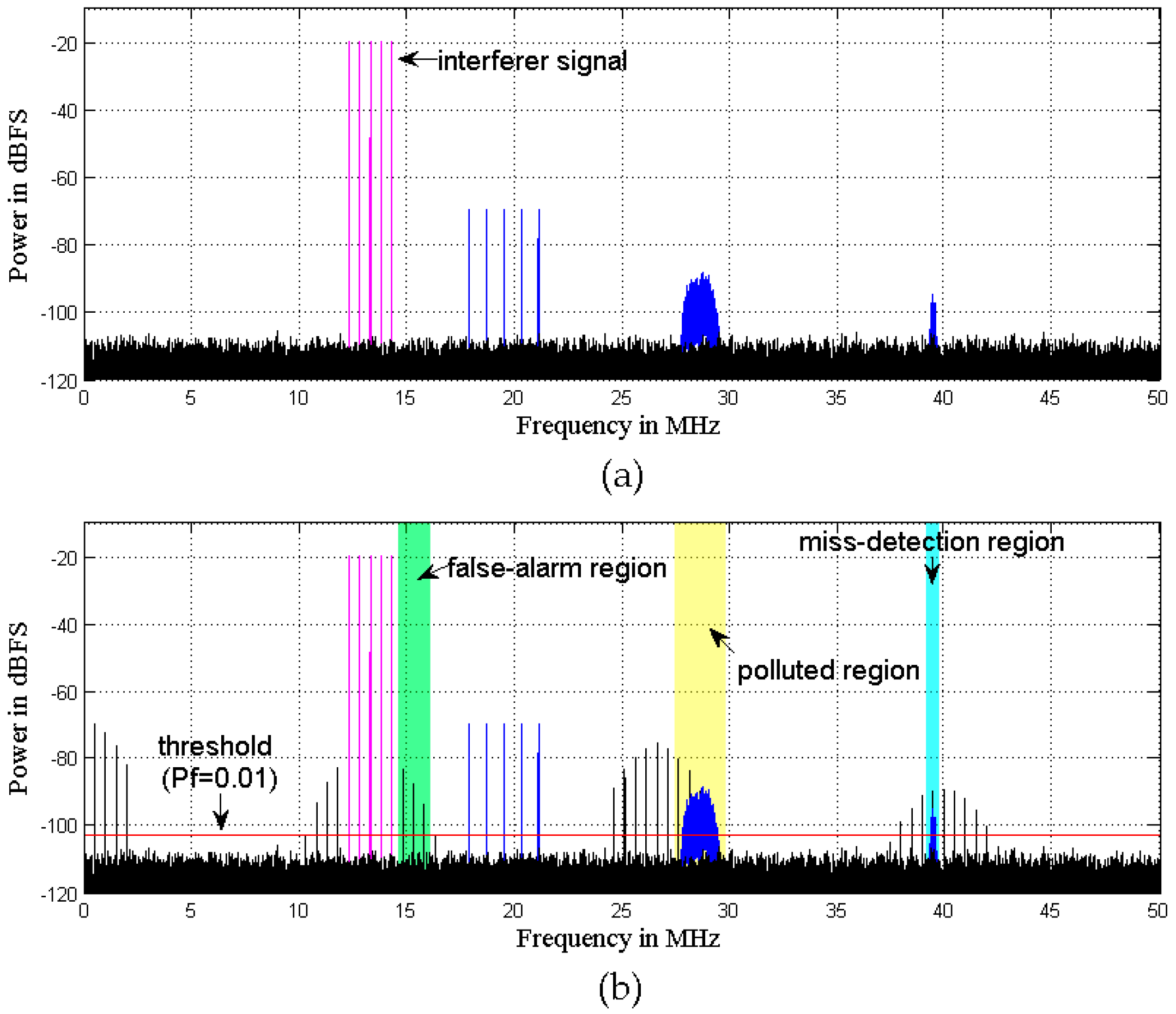
2.2. Challenges in the Spectrum Sensing Method
3. Proposed Mitigation Architecture for RF Front-End Nonlinearity
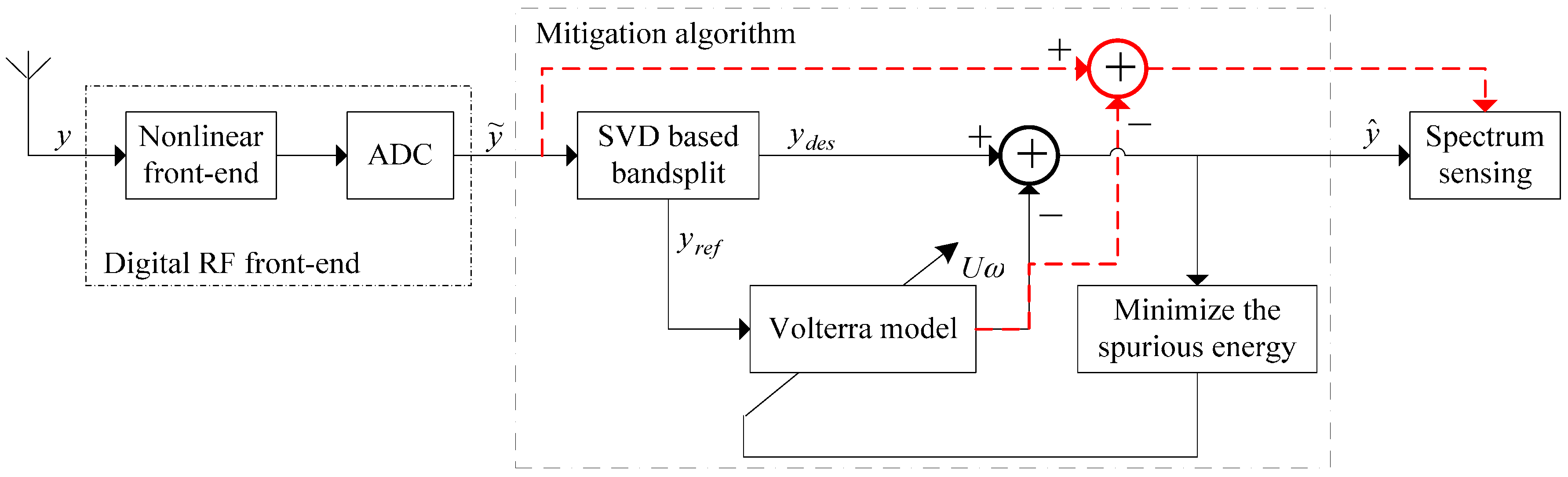
3.1. Mitigation Structure
3.2. SVD-Based Method for Bandsplit Stage
3.3. Adjustment of Volterra Coefficients
- (1)
- Create the distorted signal matrix from distorted signal according to (6);
- (2)
- Extend SVD to matrix ;
- (3)
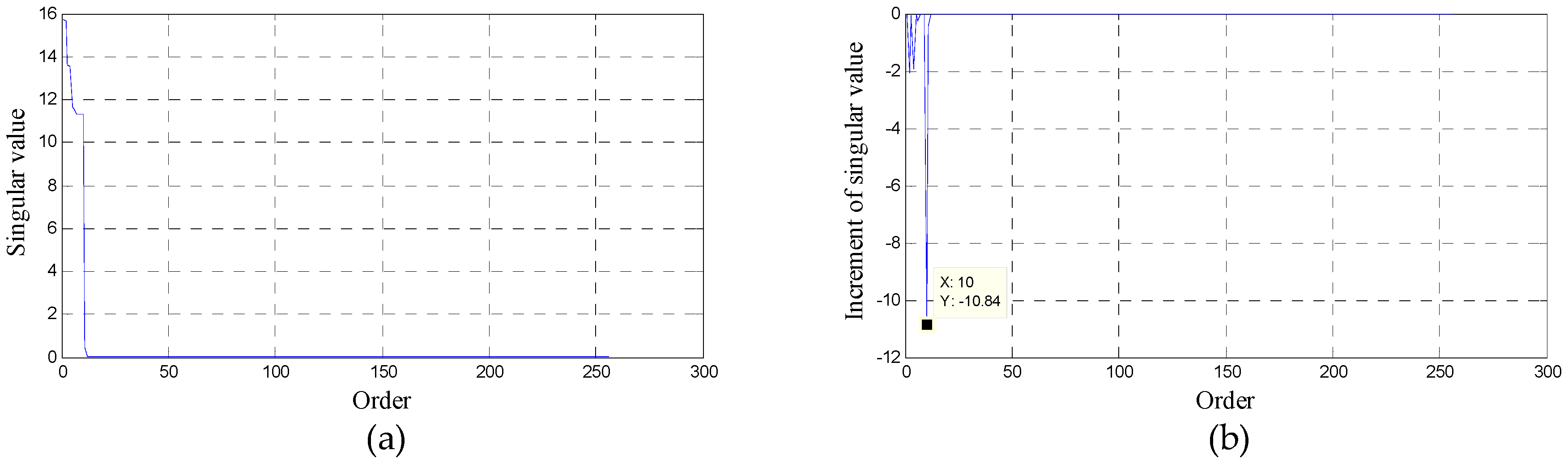
- Choose the effective order according to the minimum increment of singular values and obtain the new main diagonal matrix from (8);
- (4)
- Reconstruct the estimated interferer signal matrix according to (9), and achieve the estimated interferer signal ;
- (5)
- Achieve the main branch signal by subtracting from ;
- (6)
- Calculate from according to (10), and calculate from (16);
- (7)
- Depending on the desire to retain the interferer signal or otherwise, the mitigated output signal can be achieved by (17) or (12).
3.4. Complexity Analysis
- (1)
- Let the data length . Extending SVD to matrix by QR decomposition (The name “QR” is derived from the use of the letter Q to denote orthogonal matrices and the letter R to denote right triangular matrices.), the required calculations include: times addition, times multiplication, times division, and times square-root. Here, is the number of QR iterations.
- (2)
- iterations of subtraction are required to choose the effective order .
- (3)
- The required iterations of addition and multiplication for reconstructing the estimated interferer signal are and , respectively.
- (4)
- To obtain , iterations of multiplication are needed.
- (5)
- The required iterations of addition and multiplication of the automoment matrix generation module are and , respectively.
- (6)
- The automoment matrix inversion is implemented by LU decomposition (The name “LU” is derived from the use of the letter L to denote upper triangular matrices and the letter U to denote lower triangular matrices.). The required iterations of addition and multiplication are and , respectively.
- (7)
- To calculate , iterations of addition and iterations of multiplication are needed.
- (8)
- To calculate from (16), the required iterations of addition and multiplication are and , respectively.
- (9)
- Real-time mitigation of nonlinear distortions is performed according to (17). The required iterations for both addition and multiplication are .
4. Simulation Experiments and Analysis of Results
4.1. Verification Test Using Simulation Signals
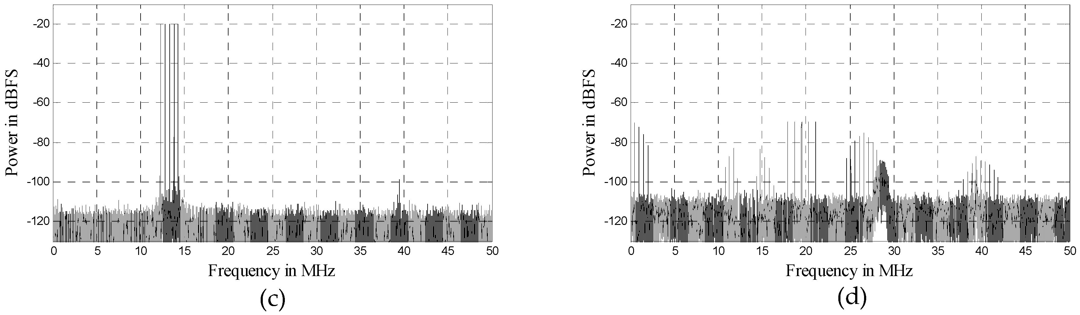
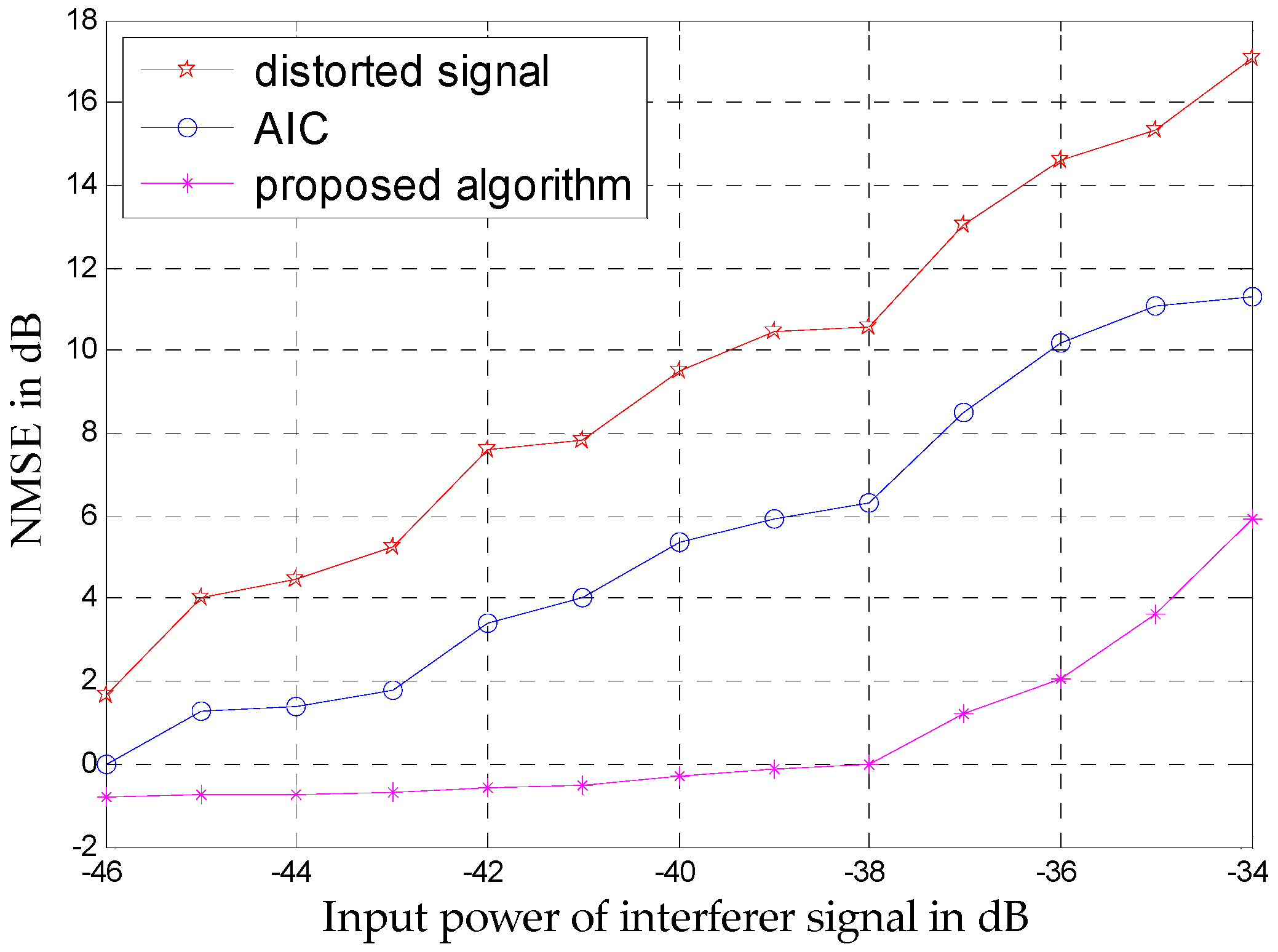
4.2. Verification Test Using Actual RF Measurements
5. Conclusions
- (1)
- A SVD-based bandsplit method is adopted instead of using bandpass/bandstop filter pairs. Thus, the coarse energy detector is not needed to achieve spectral sensing information about the level and spectral location of strong blocking signals. More importantly, the SVD-based method can effectively avoid the problem of poor compensation performance at blocker band edges due to the bandpass filter transition bands.
- (2)
- The proposed algorithm adopts the Volterra model and obtains the Volterra coefficients simply by solving a linear equation. There is no need to use AFs, and the selection of the iteration step-size as well as the problems of the convergence and complexity of LMS can be circumvented.
Acknowledgments
Author Contributions
Conflicts of Interest
Abbreviations
| CR-WSN | Cognitive Radio Wireless Sensor Network |
| RF | Radio Frequency |
| AIC | Adaptive Interference Cancellation |
| SVD | Singular Value Decomposition |
| MEMS | Micro-Electro-Mechanical Systems |
| WSN | Wireless Sensor Network |
| ISM | Industrial Scientific Medical |
| CR | Cognitive Radio |
| SU | Secondary User |
| PU | Primary User |
| LNA | Low Noise Amplifier |
| IM | Intermodulation |
| XM | Crossmodulation |
| SOI | Signal of Interest |
| DSP | Digital Signal Processing |
| AF | Adaptive Filter |
| LMS | Least Mean Square |
| FCC | Federal Communications Commission |
| BS | Base Station |
| SDR | Software-Defined Radio |
| BPF | Bandpass Filter |
| ADC | Analog-to-Digital Converter |
| DDC | Digital Down Converter |
| I/Q | In-phase/Quadrature |
| ED | Energy Detection |
| CFAR | Constant Probability of False Alarm |
| BER | Bit Error Ratio |
| SFDR | Spurious-Free Dynamic Range |
| QAM | Quadrature Amplitude Modulation |
| NMSE | Normalized Mean Squared Error |
| ROC | Receiver Operating Characteristics |
| SNR | Signal-to-Noise Ratio |
References
- Jennifer, Y.; Biswanath, M.; Dipak, G. Wireless sensor network survey. Comput. Netw. 2008, 52, 2292–2330. [Google Scholar]
- FCC. Spectrum Policy Task Force Report; Technical Report ET Docket, No. 02-155; Federal Communications Commission: Washington, DC, USA, 2002; Volume 40, pp. 147–158.
- Lu, D.-J.; Huang, X.-X. Application of cognitive radio in Wireless Sensor Networks. Bull. Adv. Technol. Res. 2009, 3, 18–22. [Google Scholar]
- Gyanendra, P.J.; Seung, Y.N.; Sung, W.K. Cognitive Radio Wireless Sensor Networks: Applications, Challenges and Research Trends. Sensors 2013, 13, 11196–11228. [Google Scholar]
- Vijay, G.; Ben Ali Bdira, E.; Ibnkahla, M. Cognition in wireless sensor networks: A perspective. IEEE Sens. J. 2011, 11, 582–592. [Google Scholar] [CrossRef]
- Bicen, A.O.; Gungor, V.C.; Akan, O.B. Delay-sensitive and multimedia communication in cognitive radio sensor networks. Ad Hoc Netw. 2012, 10, 816–830. [Google Scholar] [CrossRef]
- Han, J.A.; Jeon, W.S.; Jeong, D.G. Energy-efficient channel management scheme for cognitive radio sensor networks. IEEE Trans. Veh. Technol. 2011, 60, 1905–1910. [Google Scholar] [CrossRef]
- Li, B.; Sun, M.-W.; Li, X.-F. Energy detection based spectrum sensing for cognitive radios over time-frequency doubly selective fading channels. IEEE Trans. Signal Process. 2015, 63, 402–417. [Google Scholar] [CrossRef]
- Subramaniam, S.; Reyes, H.; Kaabouch, N. Spectrum occupancy measurement: An autocorrelation based scanning technique using USRP. In Proceedings of the 2015 IEEE 16th Annual Wireless and Microwave Technology Conference (WAMICON), Cocoa Beach, FL, USA, 13–15 April 2015.
- Reyes, H.; Subramaniam, S.; Kaabouch, N.; Wen, C.-H. A spectrum sensing technique based on autocorrelation and Euclidean distance and its comparison with energy detection for cognitive radio networks. Comput. Electr. Eng. 2015, 52, 319–327. [Google Scholar] [CrossRef]
- Moghaddam, S.S.; Kamarzarrin, M. A Comparative Study on the Two Popular Cognitive Radio Spectrum Sensing Methods: Matched Filter Versus Energy Detector. Am. J. Mob. Syst. Appl. Serv. 2015, 1, 132–139. [Google Scholar]
- Xu, S.; Zhao, Z.; Shang, J. Spectrum Sensing Based on Cyclostationarity. In Proceedings of the IEEE Workshop on Power Electronics and Intelligent Transportation System (PEITS), Guangzhou, China, 2–3 August 2008; pp. 171–174.
- Zeng, Y.; Liang, Y.-C. Eigenvalue-based spectrum sensing algorithms for cognitive radio. IEEE Trans. Commun. 2009, 57, 1784–1793. [Google Scholar] [CrossRef]
- Wang, Y.-H.; Li, Y.-H.; Yuan, F.; Yang, J. A cooperative spectrum sensing scheme based on trust and fuzzy logic for cognitive radio sensor networks. Int. J. Comput. Sci. Issues 2013, 10, 275–279. [Google Scholar]
- Allén, M.; Marttila, J.; Valkama, M.; Makinen, S.; Kosunen, M.; Ryynanen, J. Digital linearization of direct-conversion spectrum sensing receiver. In Proceedings of the IEEE Global Conference on Signal Information Processing, Austin, TX, USA, 3–5 December 2013; pp. 1158–1161.
- Grimm, M.; Allen, M.; Marttila, J.; Valkama, M.; Thoma, R. Joint mitigation of nonlinear RF and baseband distortions in wideband direct-conversion receivers. IEEE Trans. Microw. Theory Tech. 2014, 62, 166–182. [Google Scholar] [CrossRef]
- Razavi, B. Cognitive radio design challenges and techniques. IEEE J. Solid-State Circuits 2010, 45, 1542–1553. [Google Scholar] [CrossRef]
- Mahrof, D.; Klumperink, E.A.M.; Haartsen, J.C.; Nauta, B. On the effect of spectral location of interferers on linearity requirements for wideband cognitive radio receivers. In Proceedings of the DYSPAN, Singapore, 6–9 April 2010; pp. 1–9.
- Rebeiz, E.; Shahed, A.; Valkama, M.; Cabric, D. Suppressing RF front-end nonlinearities in wideband spectrum sensing. In Proceedings of the CROWNCom, Washington, DC, USA, 8–10 July 2013; pp. 87–92.
- Rebeiz, E.; Ghadam, A.S.H.; Valkama, M.; Cabric, D. Spectrum Sensing Under RF Non-Linearities Performance Analysis and DSP-Enhanced Receivers. IEEE Trans. Signal Process. 2015, 63, 1950–1964. [Google Scholar] [CrossRef]
- Fettweis, G.; Lohning, M.; Petrovic, D.; Windisch, M.; Zillmann, P.; Rave, W. Dirty RF: A new paradigm. In Proceedings of the IEEE 16th International Symposium on Personal, Indoor and Mobile Radio Communications (PIMRC), Berlin, Germany, 11–14 September 2005; pp. 2347–2355.
- Valkama, M.; Ghadam, A.S.H.; Anttila, L.; Renfors, M. Advanced digital signal processing techniques for compensation of nonlinear distortion in wideband multicarrier radio receivers. IEEE Trans. Microw. Theory Tech. 2006, 54, 2356–2366. [Google Scholar] [CrossRef]
- Grimm, M.; Sharma, R.K.; Hein, M.; Thomä, R. DSP-based mitigation of RF front-end non-linearity in cognitive wideband receivers. Frequenz J. RF Eng. Telecommun. 2012, 66, 303–310. [Google Scholar] [CrossRef]
- Allén, M.; Marttila, J.; Valkama, M.; Grimm, M.; Thomä, R. Digital post-processing based wideband receiver linearization for enhanced spectrum sensing and access. In Proceedings of the 9th International Conference on Cognitive Radio Oriented Wireless Networks and Communications (CROWNCOM), Oulu, Finland, 2–4 June 2014; pp. 520–525.
- Taparugssanagorn, A.; Umebayashi, K.; Lehtomaki, J.; Pomalaza-Raez, C. Analysis of the effect of nonlinear low noise amplifier with memory for wideband spectrum sensing. In Proceedings of the 1st International Conference on 5G for Ubiquitous Connectivity (5GU), Akaslompolo, Finland, 26–28 November 2014; pp. 87–91.
- Safatly, L.; El-Hajj, A.; Kabalan, K.Y. Blind and robust spectrum sensing based on RF impairments mitigation for cognitive radio receivers. In Proceedings of the International Conference on High Performance Computing & Simulation (HPCS), Bologna, Italy, 21–25 July 2014; pp. 820–824.
- Dupleich, D.; Grimm, M.; Schlembach, F.; Thoma, R.S. Practical aspects of a digital feedforward approach for mitigating non-linear distortions in receivers. In Proceedings of the 11th International Conference on Telecommunication in Modern Satellite, Cable and Broadcasting Services (TELSIKS), Nis, Serbia, 16–19 October 2013; pp. 170–177.
- Axell, E.; Leus, G.; Larsson, E.G.; Poor, H.V. Spectrum sensing for cognitive radio: State-of-the-art and recent advances. IEEE Signal Process. Mag. 2012, 29, 101–116. [Google Scholar] [CrossRef]
- Rugh, W.J. Nonlinear System Theory: The Volterra/Wiener Approach; The John Hopkins University Press: Baltimore, MD, USA, 1981. [Google Scholar]
- Dobrzanska, A.; Ordynski, J. Digital distortion compensation for wideband direct digitization RF receiver. In Proceedings of the 13th International Conference on New Circuits and Systems Conference (NEWCAS), Grenoble, France, 7–10 June 2015; pp. 1–4.
- Haykin, S. Adaptive Filter Theory, 3rd ed.; Prentice-Hall: Upper Saddle River, NJ, USA, 1996. [Google Scholar]
- Akan, O.B.; Karli, O.B.; Ergul, O. Cognitive Radio Sensor Networks. IEEE Netw. 2009, 7, 34–40. [Google Scholar] [CrossRef]
- Murty, R.; Chandra, R.; Moscibroda, T.; Bahl, P. SenseLess: A database-driven white spaces network. IEEE Trans. Mob. Comput. 2012, 11, 189–203. [Google Scholar] [CrossRef]
- Yang, W.-X.; Jiang, J.-S. Study on the singular entropy of mechanical signal. Chin. J. Mech. Eng. 2000, 36, 9–13. [Google Scholar] [CrossRef]
- Zhang, C.-M.; Yao, S. On the research of weight iterative improvement method for morbid state linear systems. J. Anqing Teach. Coll. (Nat. Sci.) 2004, 10, 78–79. [Google Scholar]


| Operator | Computational Complexity |
|---|---|
| Addition | |
| Multiplication | |
| Division | |
| square-root |
© 2016 by the authors; licensee MDPI, Basel, Switzerland. This article is an open access article distributed under the terms and conditions of the Creative Commons Attribution (CC-BY) license (http://creativecommons.org/licenses/by/4.0/).
Share and Cite
Hu, L.; Ma, H.; Zhang, H.; Zhao, W. Mitigating RF Front-End Nonlinearity of Sensor Nodes to Enhance Spectrum Sensing. Sensors 2016, 16, 1999. https://doi.org/10.3390/s16121999
Hu L, Ma H, Zhang H, Zhao W. Mitigating RF Front-End Nonlinearity of Sensor Nodes to Enhance Spectrum Sensing. Sensors. 2016; 16(12):1999. https://doi.org/10.3390/s16121999
Chicago/Turabian StyleHu, Lin, Hong Ma, Hua Zhang, and Wen Zhao. 2016. "Mitigating RF Front-End Nonlinearity of Sensor Nodes to Enhance Spectrum Sensing" Sensors 16, no. 12: 1999. https://doi.org/10.3390/s16121999