2.1. Cytometric Pulse Generation and Fluorescence Spectral Overlap
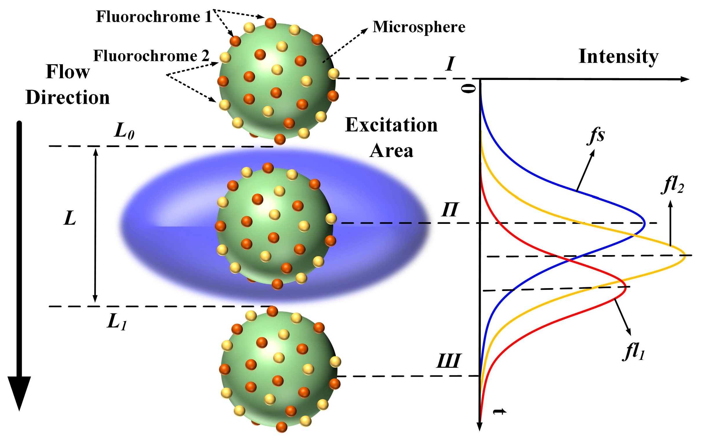
In flow cytometry, fluorescence signals are often referred to as “cytometric pulses” or “waveforms”, because they are the result of the rapid transit of a fluorescently labeled cell through a tightly focused laser beam with a Gaussian profile. As shown in
Figure 1, the microsphere moves along the flow direction through the excitation area (blue ellipsoid,
Figure 1). A Gaussian-like trace reflects the resulting signal, where the forward-scattered emission begins to increase at time
Ι (the microsphere flows across the upper limb
L0 into the excitation area), peaks at time
Π, and decreases as the microsphere moves from time
Π to time
Ш (the microsphere flows across the lower limb
L1).
Therefore, the original signals
fl1 and
fl2 are mathematically expressed as:
where
fs is the forward-scattered pulse;
K,
A, and
B are constants representing the heights of the curve peaks;
t0,
t0 − Δ
t1, and
t0 − Δ
t2 represent the peak positions; and σ represents the curve width.
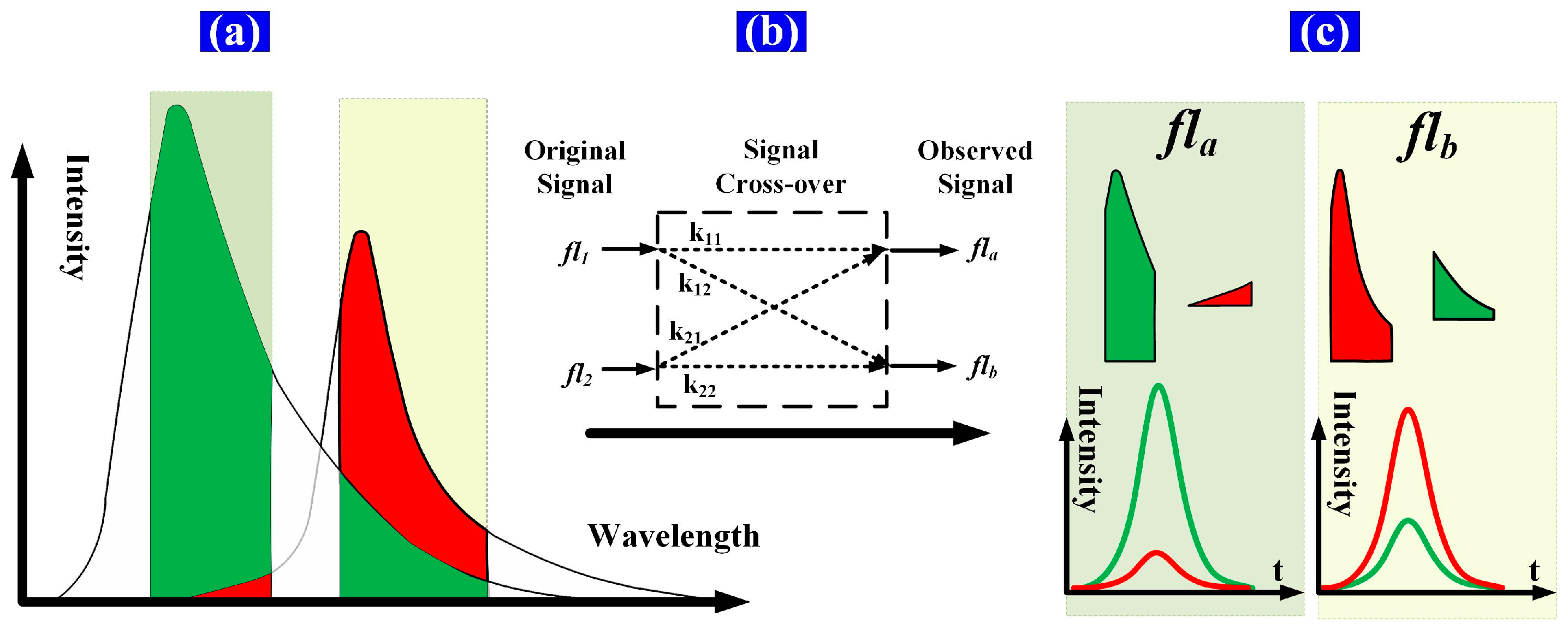
Spectral overlap, or “spillover”, results from the use of fluorescent dyes that are measurable in more than one detector. This spillover is correlated by a constant known as the spillover coefficient. Spectral overlap is illustrated schematically in
Figure 2. Two fluorochromes with different lifetimes are excited simultaneously and then detected using detector channels having fixed bandwidths. The time-intensity Gaussian-like cytometric pulses (
fs,
fl1, and
fl2) are generated as the microspheres flow through the extinction area. Then, the spectrum of each fluorochrome is detected by a different detector channel having a fixed bandwidth. Both the peak value and the peak location of the detected signal (time-intensity cytometric pulse) of each detector channel are influenced by the spectral overlap due to the different fluorochrome lifetimes. That is, the time delays between the observed fluorescence signals (
fla,
flb) and
fs are influenced by the spectral overlap [
12,
13,
14,
15].
In addition, considering the influence of autofluorescence, the dim expression of the exogenous fluorophores adds a number of spectral overlap. Autofluorescence is due to many cellular constituents, rather than a single fluorochrome with a single exponential decay, and it is difficult to distinguish the influence of this behavior from the observed fluorescence spectrum. However, the autofluorescence is dependent on certain cell constituents, it is relatively stable, and its dim intensity barely shifts the peak locations of the fluorescence pulse signals, even with multi-exponential decay. Therefore, the autofluorescence can be fully handled with the emission fluorescence. In what follows, the autofluorescence overlap are regarded as elements of the emission fluorescence for the lifetime calculations of cells labeled with single- or two-color fluorochromes.
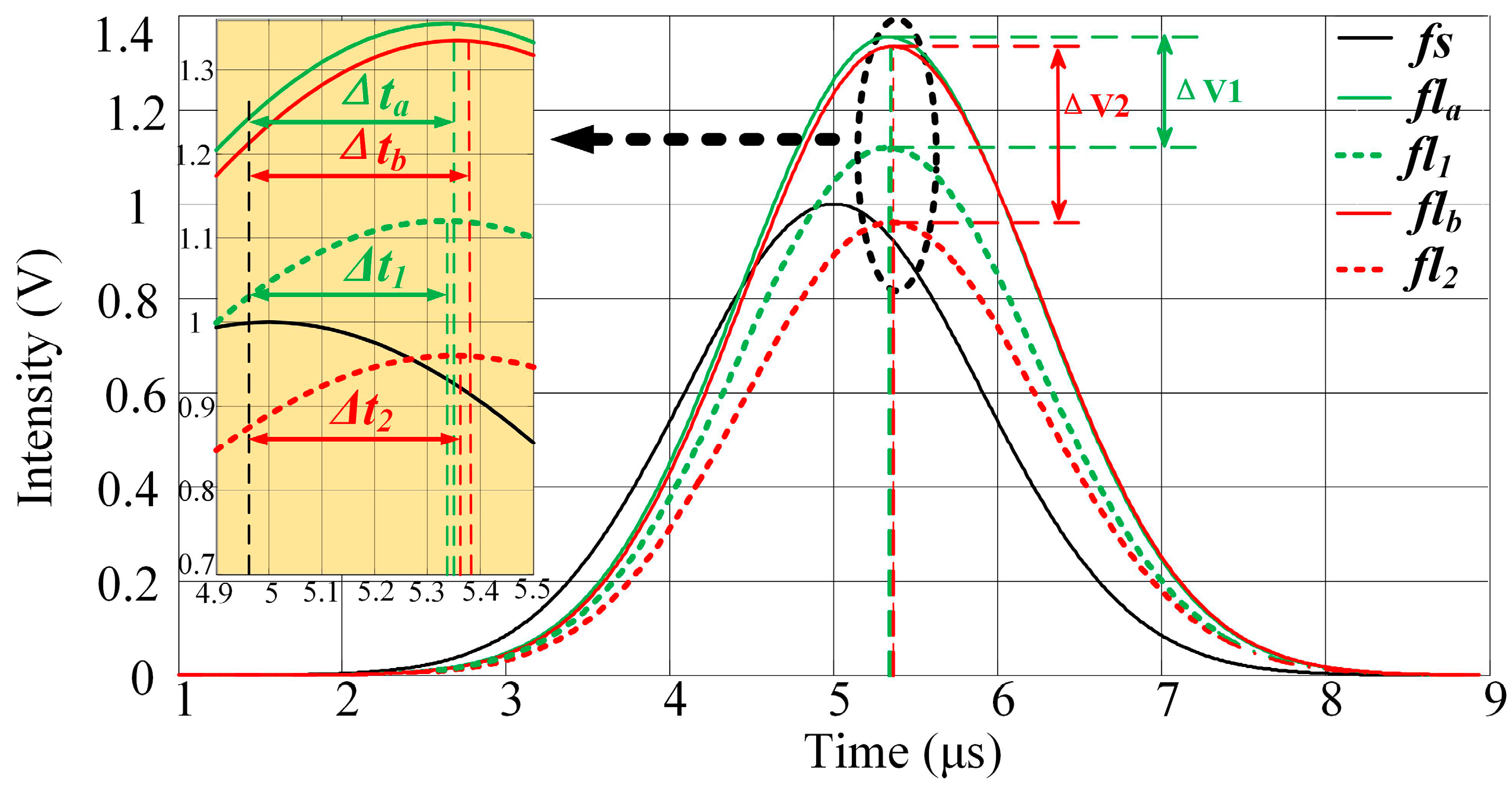
The signals after crossover (
fla,
flb) are shown in
Figure 3 and described by Equation (2) below. The expected results of the detector channels are
k11fl1 and
k22fl2. However, the peak values and peak locations of the observed signals are influenced by signal crossover. The peak values of the observed signals increase with the addition of parts of the crossover signals. The peak-value errors (
Epa,
Epb) introduced through crossover can be calculated using Equation (3). Meanwhile, the peak locations of
fl1 and
fl2 differ, and the
fla and
flb peak locations move to the left or right when parts of the crossover signals are added. The peak-location errors (
Eta,
Etb) introduced through crossover can be calculated using Equation (4):
Here,
Pa,
P1,
Pb, and
P2 are the peak values of
fla,
fl1,
flb, and
fl2, respectively.
The peak-value errors and the pulse time delay errors (Δ
ta − Δ
t1, Δ
tb − Δ
t2: the time delays of the peak locations between
fs and the fluorescence pulses (
fl1,
fl2,
fla and
flb)) introduced by the signal crossover are shown in
Figure 3. It is apparent that Δ
V1 and Δ
V2 are significantly larger than Δ
ta − Δ
t1 and Δ
tb − Δ
t2. Note that the peak values of different fluorescence signals can vary widely and fluorescence intensity measurements are impacted by nonlinearity. Therefore, the peak-value errors introduced by crossover are typically large and are difficult to amend. On the other hand, the differences in the pulse time delays between the different fluorescence pulses are significantly smaller. The pulse time delays vary little with signal crossover. Therefore, the influence of crossover can be decreased be using the pulse time delay as a parameter when representing the fluorescence pulse.
2.2. Fluorescence Pulse Time-Delay Estimation
The time delay between the observed fluorescence signal and the forward-scattered signal includes the lifetime and delay introduced by the hardware [
3]. However, only the fluorescence lifetime is relevant for removing the crossover signal from the observed signal in the following sections. Therefore, it is necessary to determine the relationship between the time delay and lifetime. We assume that the fluorescent light is emitted in accordance with the single exponential decay model. The fluorescent-light signal can be expressed as a convolution of the forward-scattered light and the single exponential decay model, such that:
where
L_fl is the fluorescent-light pulse;
L_fs is the forward-scattered light pulse;
K0 is the signal intensity; and τ is the fluorescence lifetime. Then, we can conclude that the phase shift between
L_fl and
L_fs is the phase of
: arctan(ωτ). Therefore, the time delay between the fluorescent-light pulse and the forward-scattered light pulse is equal to τ.
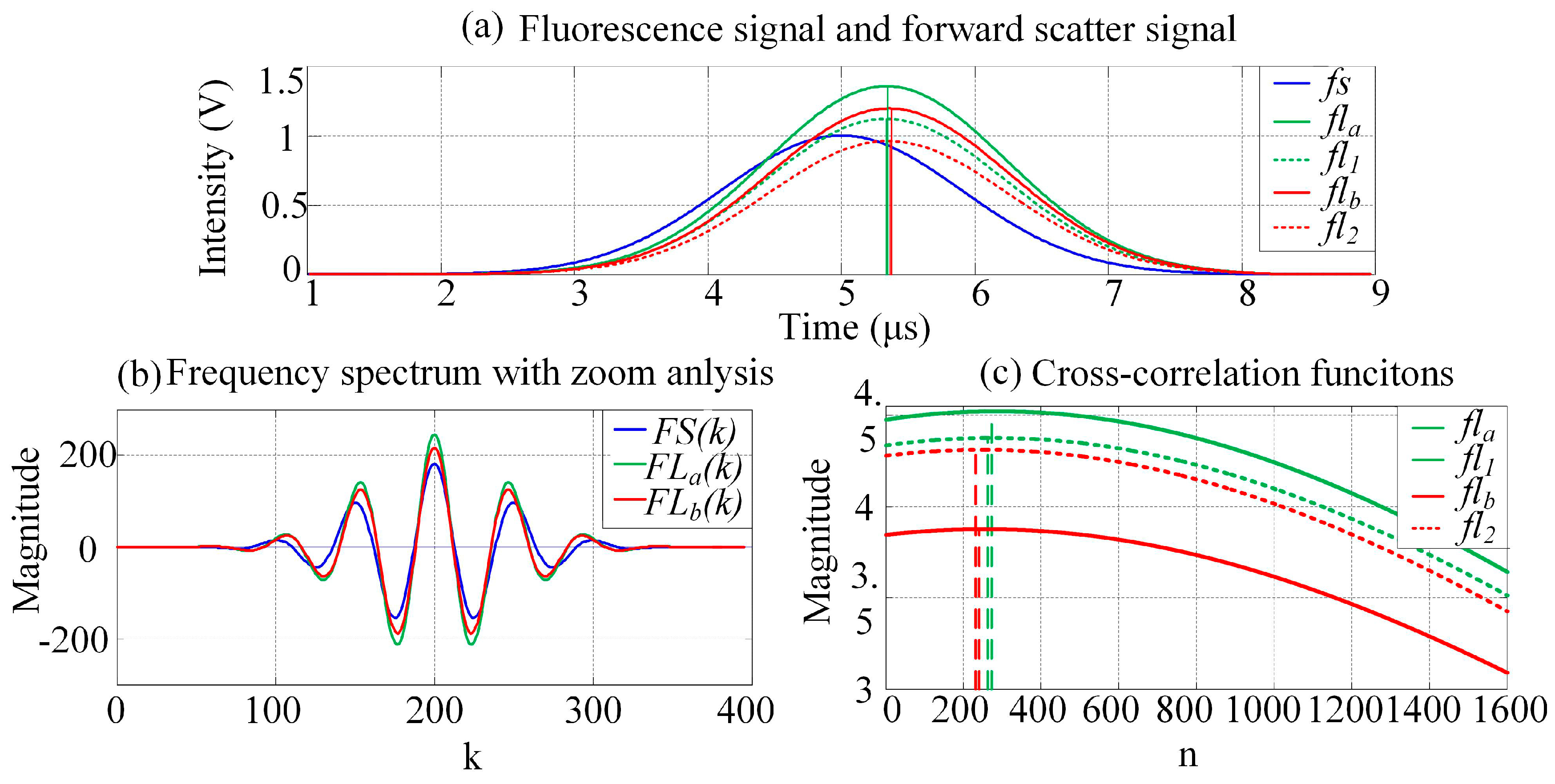
To estimate the time delay of output pulse signals from circuit systems, the cross-correlation function algorithm is applied to restrain the influence of the noise. However, the estimation accuracy with a traditional cross-correlation function is limited by the time interval between adjacent points in the pulse signal, i.e., by the sampling frequency of the analog-to-digital converter (ADC). In this work, zoom analysis of the frequency spectrum within the scope of a certain frequency is executed using the modified chirp Z-transform (MCZT) method, so as to acquire the frequency spectral information with high resolution. The frequency resolution is higher with larger N1, however, more time would be taken for computing. The frequency spectral information is neither limited by the pulse signal length nor the ADC sampling frequency. The fine interpolation of the correlation peak (FICP) algorithm is then used to improve the resolution of the time-domain cross-correlative function. This method avoids modulating the laser at different frequencies and effectively presents a platform for lifetime detection that is easier to practically implement on any standard flow cytometer.
Assuming that the forward-scattered pulse signal
fs(
n) and the fluorescence pulse signal
flm(
n) are data sequences containing
N points, the corresponding zoomed frequency spectra (
FS(
k) and
FLm(
k), respectively) are described by the transform:
where
m = 1, 2, a, b and
k = 0, 1, …,
N − 1.
Based on the sampling theorem,
FS(
k) and
FLm(
k) are periodic functions and the cycle is
N1, while the first and last parts of the functions are conjugate symmetric. With the FICP analysis, the sampling frequency is raised to
N2/
N1 times the initial sampling frequency, when the frequency spectrum cycle is extended from
N1 to
N2 with the insertion of zero. That is, the resolution of the time delay between
fs(
n) and
flm(
n) in the time domain is increased to
N2/
N1 times for the same number of calculations. The complete cross-correlation frequency spectrum is constructed as:
The time delays are distributed within a certain limited range and, similarly, the time delays between
fs(
n) and
flm(
n) fall into a certain limited range. In this case, only a finite number of the first and last parts of the points are required for the calculation. The first and last parts of the cross-correlation function in the time domain,
r1(
n) and
r2(
n), respectively, are calculated from Equations (8) and (9), respectively, as follows:
where
m = 1, 2,
a,
b and
k = 0, 1,
…,
N − 1.
N2 is the length of both
FS(
k) and
FLm(
k) after the zeros are inserted.
The value of
N2 is set arbitrarily, and the resolution of
r1(
n) and
r2(
n) is increased by
N2/
N1. Meanwhile, the integrated cross-correlation function in the time domain
r(
n) is constructed with
r1(
n) and
r2(
n), such that:
The resolution of the cross-correlation peak is improved by increasing the interpolation multiple of the frequency spectrum. That is, the computational accuracy of the time-delay estimation is higher with FICP, particularly for pulse signals of low sampling frequency.
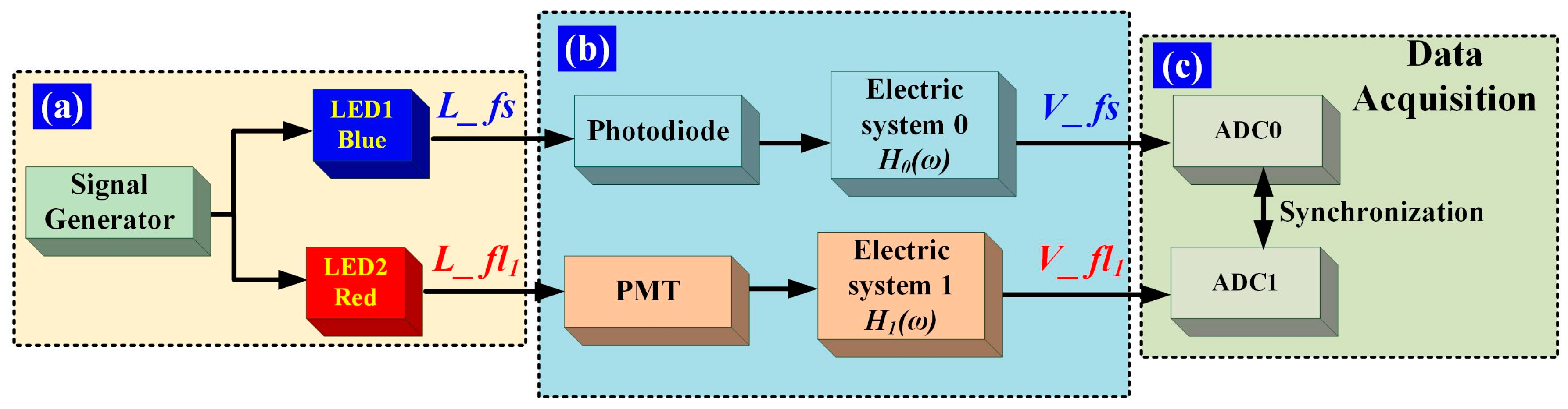
It is necessary to correct for the inherent time delay introduced by the hardware variables, such as the differences in the photoelectric detector, circuitry, and cable. The time delay introduced by the hardware can be eliminated via calibration, which is performed as shown in
Figure 4. Two light-emitting diodes (LEDs) are used as light sources and are pulsed synchronously by a standard function generator with Gaussian waveforms. As shown in
Figure 4a, the Gaussian-shaped light pulses
L_fs and
L_fl1 are used to represent the forward-scattered light pulse and the fluorescent-light pulse of a flow cytometer, respectively.
L_fs and
L_ fl1 are synchronous with the same pulsed signal.
Figure 4b shows the photovoltaic conversion and the electric systems. The corresponding electrical pulse signal is presented in terms of
V_fs and
V_fl1, and then converted to digital signals using ADCs labeled ADC0 and ADC1, respectively, as illustrated in
Figure 4c. The ADC0 and ADC1 clock signals are provided by one crystal oscillator, to ensure that
V_fs and
V_ fl1 are converted simultaneously. The time delay between
V_fs and
V_fl1 can be acquired and taken as the time delay introduced by the photovoltaic conversion and electric systems.
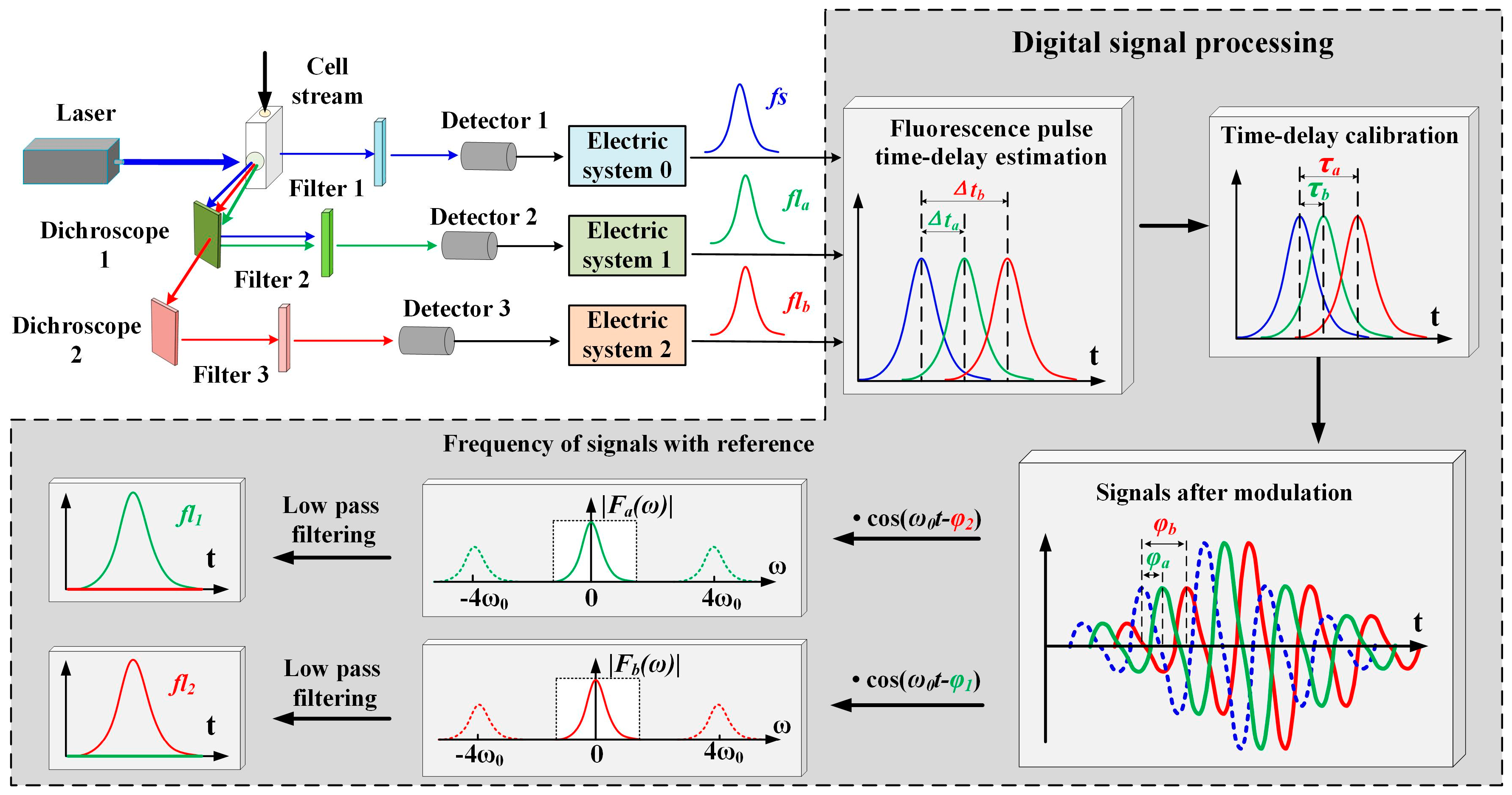
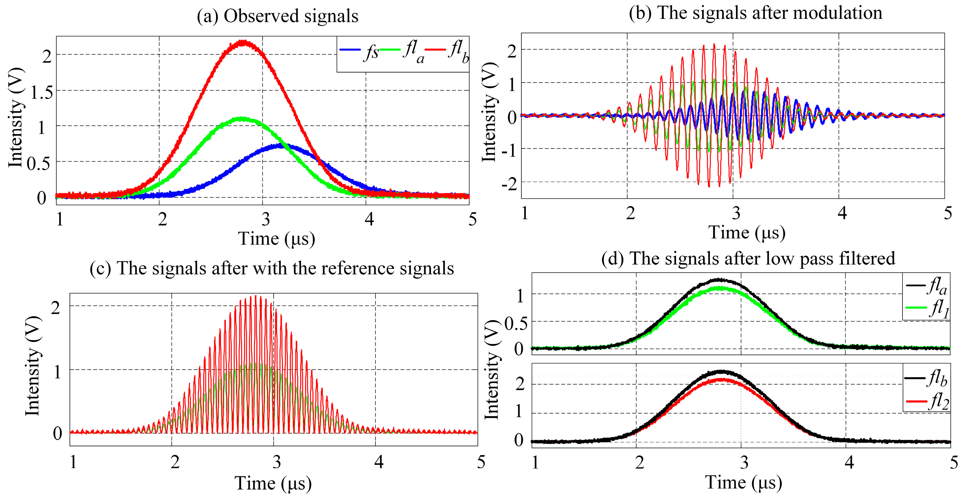
2.3. Representation of Spectrally Overlapping Fluorescence Signals
Spectrally overlapping fluorescence signals are represented using the process shown in
Figure 5. The cells are analyzed as they intersect a laser excitation beam. The fluorescence is measured orthogonally to the laser beam-cell stream intersection point in the flow chamber, using a dichroscope, a filter, a signal detector, and an electric system [
16]. The time delays (Δ
ta, Δ
tb) of the fluorescence pulses (
fla,
flb) are estimated using the above-mentioned FICP arithmetic. As mentioned above, the forward-scattered signal and the fluorescence signal are Gaussian in shape. For a generated signal,
fs,
fla, and
flb can be expressed as shown in Equation (11) [
16,
17,
18].
where,
K1,
C1, and
D1 are the signal intensity,
t0' is the center moment of the scattered signal; τ
a and τ
b are the calculated lifetimes of
fla and
flb, respectively; and
h0(
t),
h1(
t), and
h2(
t) are the transfer functions of electric systems 0, 1, and 2, respectively.
The individual lifetimes τ1 and τ2 are acquired so as to express the phase shift introduced by the lifetime. In order to acquire the individual lifetime components of each fluorochrome, the cells are labeled with one kind of fluorochrome only and tested separately. Then, fl1 and fl2 are detected, and τ1 and τ2 are acquired, respectively, using the MCZT and FICP techniques.
The signals after modulation (
fs_mod,
fla_mod, and
flb_mod) are artificially created using a digital signal processing method, as shown in Equation (12). The modulating signal is a cosine function, and the phase shifts of
fla and
flb introduced by τ
a and τ
b are ϕ
a = arctan(ω
0τ
a) and ϕ
b = arctan(ω
0τ
b), respectively. Considering the relationship between the observed (
fla,
flb) and original signals (
fl1,
fl2), the expressions given in Equation (13) can be acquired. Hence, the phase shifts introduced by τ
1 and τ
2 are ϕ
1 = arctan(ω
0τ
1) and ϕ
2 = arctan(ω
0τ
2), respectively.
Here, K2, C2, C3, C4, D2, D3, and D4 are the signal intensities; t0 is the center moment of fs_mod; and ω0 is the angular frequency of the modulation.
The aim of PTDE is to transform the observed summation signal, which is measured experimentally, into a signal that is dependent on one fluorophore only. Nullifying one of the fluorescence signals by exploiting the fluorophore lifetime is necessary for this to occur. Nullification is accomplished by mixing a cosine reference signal, which is performed by altering the reference signal phase. The reference signal has the same angular frequency as the modulating signal and the reference phase is shifted by an amount ϕ
ref1 = ϕ
2 or ϕ
ref2 = ϕ
1. The mixing results (
fla_mix,
flb_mix) are expressed as:
Finally, the original fluorescence signal (
fl1,
fl2) can be obtained via low-pass filtering, as expressed in Equation (15). Both signals are resolved, but with a loss in amplitude [1/2cos(ϕ
1 − ϕ
2)]:


