
Context-Aware Fusion of RGB and Thermal Imagery for Traffic Monitoring

Abstract
:1. Introduction
2. Related Work
3. Context-Based Image Quality Parameters
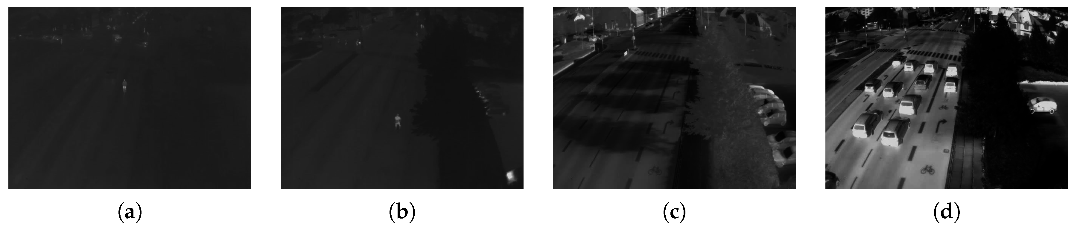
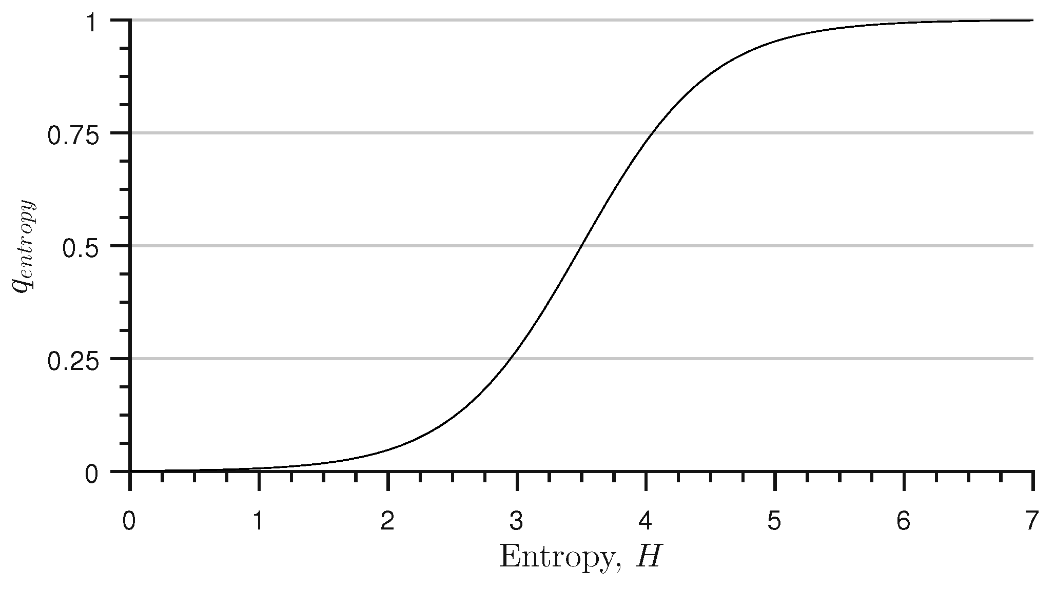
3.1. Predictable Thermal Image Quality Characteristics
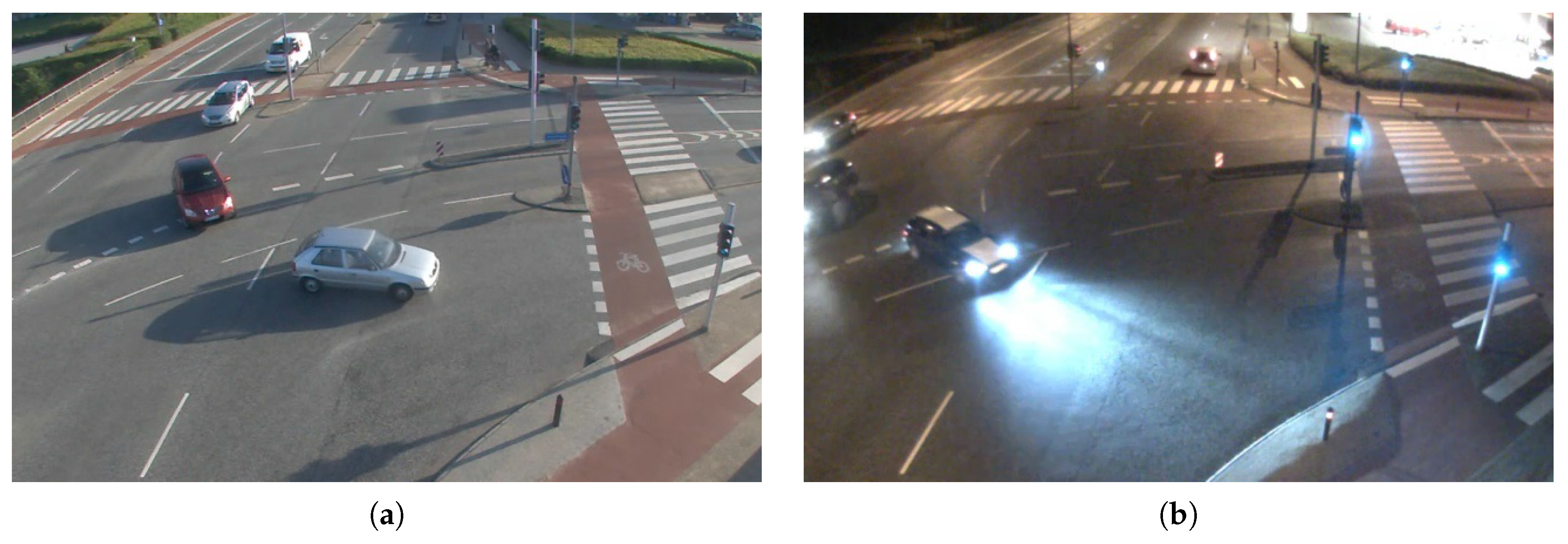
3.2. Predictable RGB Image Quality Characteristics
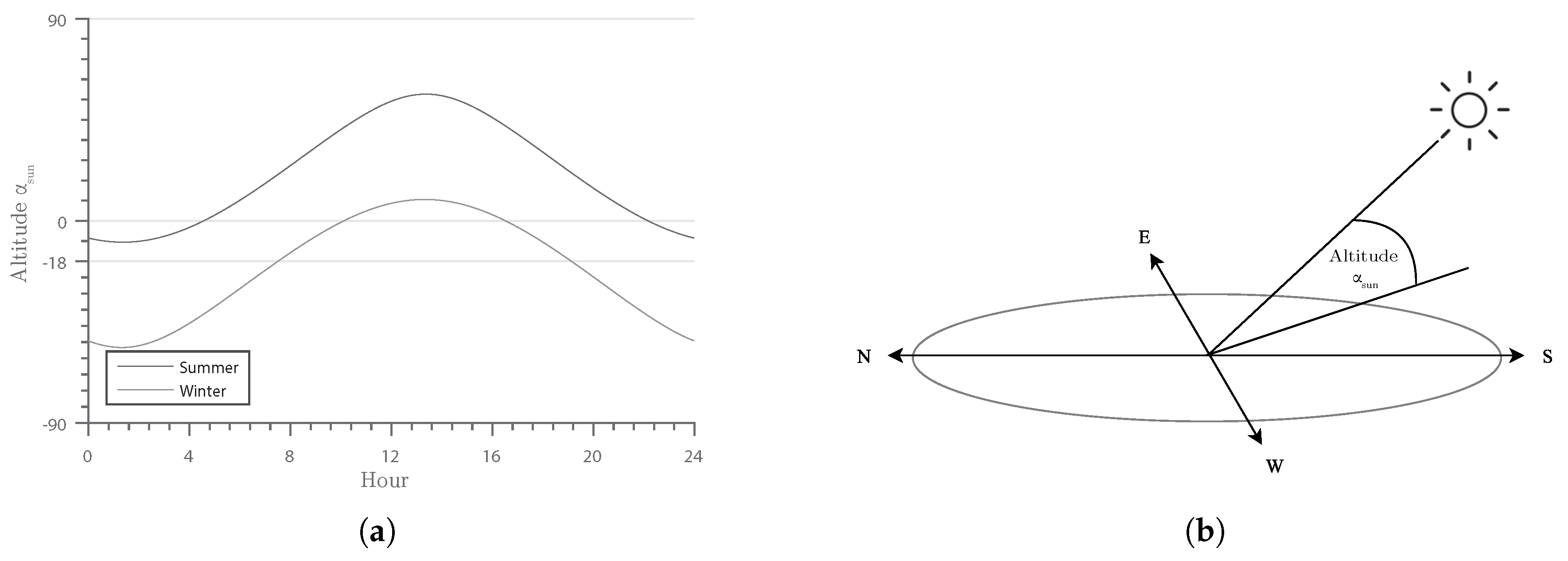
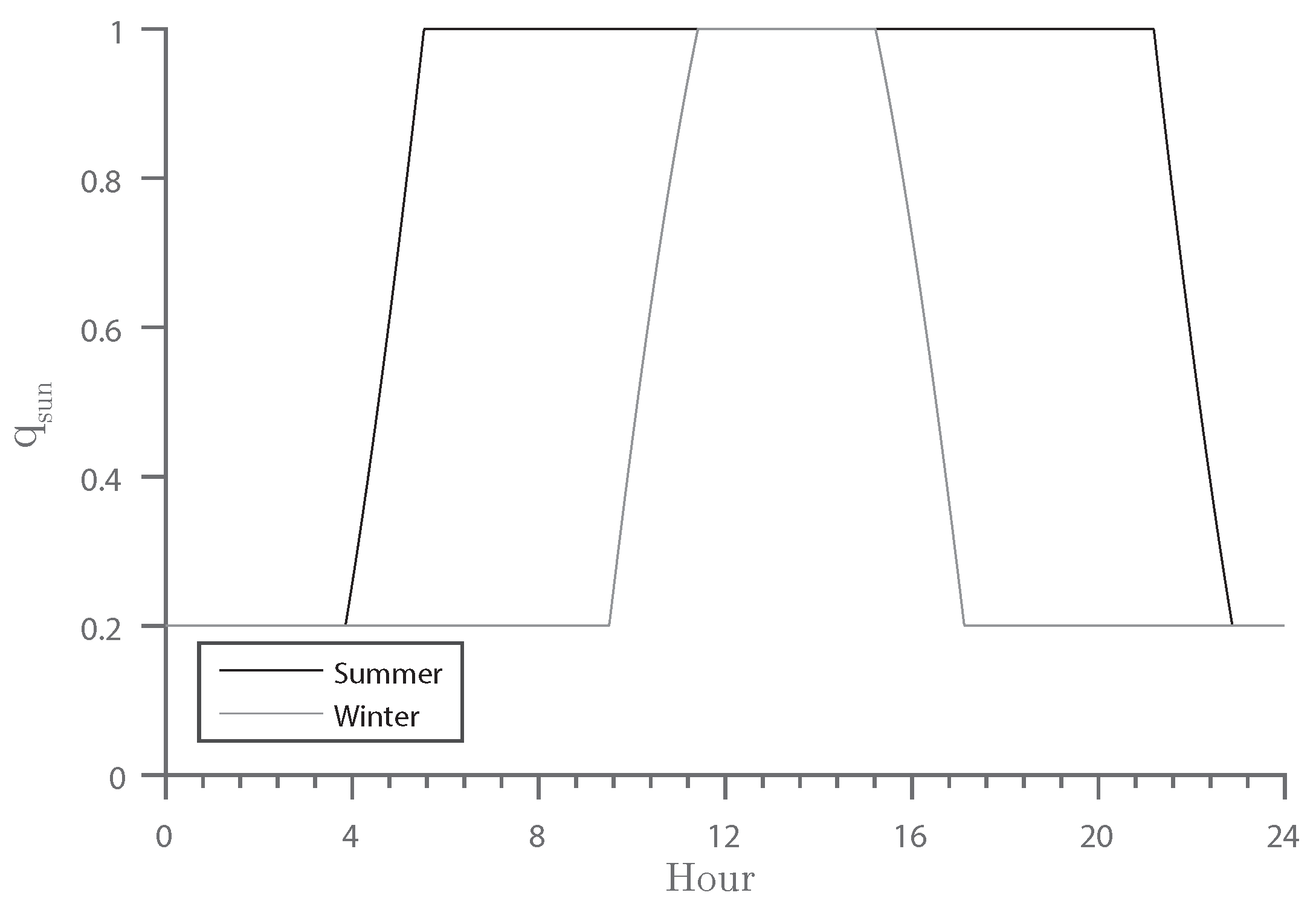
3.2.1. Illumination
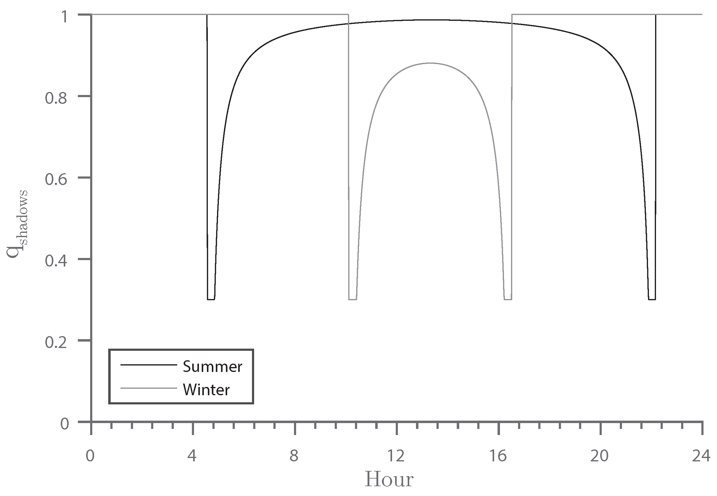
3.2.2. Shadows
3.2.3. Weather Conditions
3.3. Unpredictable Image Quality Characteristics
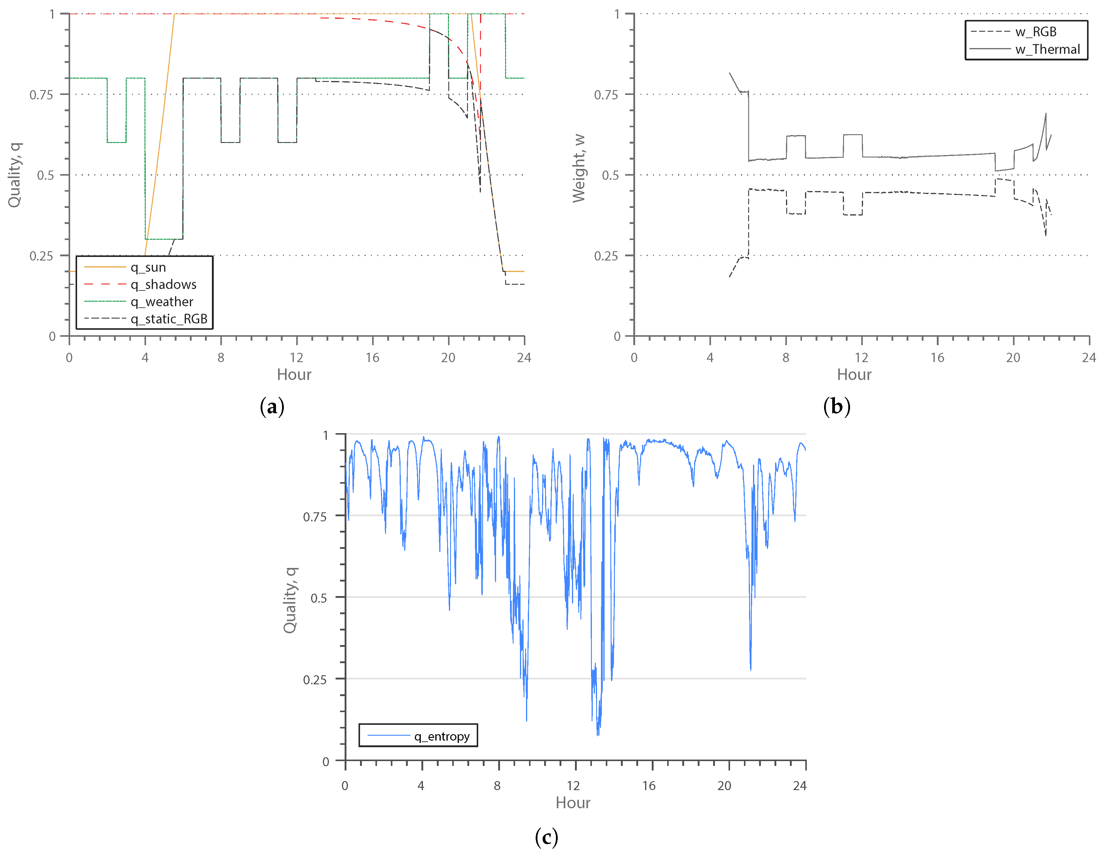
3.4. Combined Quality Characteristics
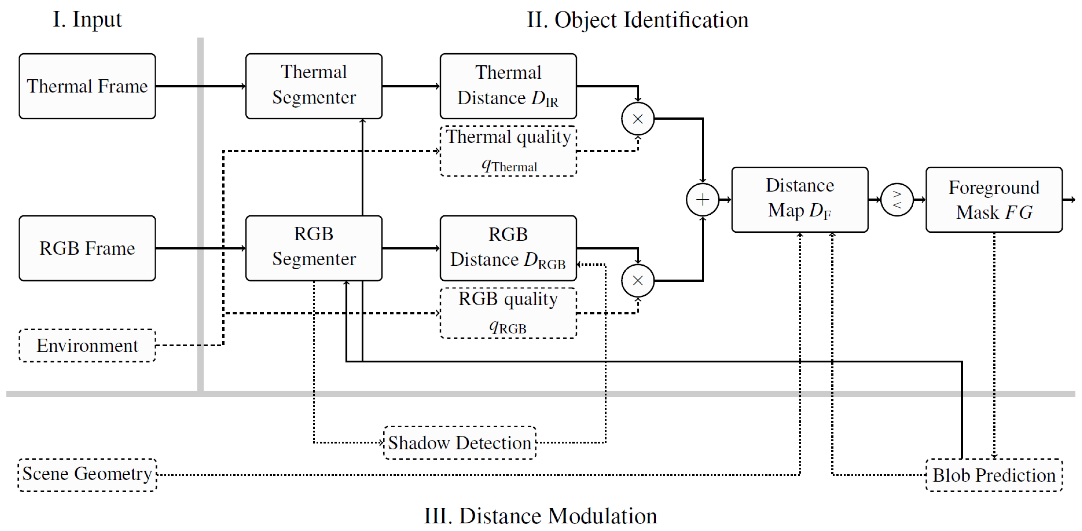
4. Context-Based Fusion
5. Segmentation Algorithm
6. Application to Traffic Monitoring
6.1. Shadow Detection
6.2. Blob Prediction
6.3. Scene Geometry-Based Knowledge
7. Experiments
7.1. The Datasets
7.2. Performance Metrics
7.3. Quantitative Results
- RGB: individual processing of the RGB modality by the proposed method.
- Thermal: individual processing of the thermal modality by the proposed method.
- RGBT: pixel-wise, naive (not context-aware) fusion of RGB and thermal streams.
- Select: confidence-based selection as presented by Serrano-Cuerda et al. [11]
7.4. Special Situation Performance
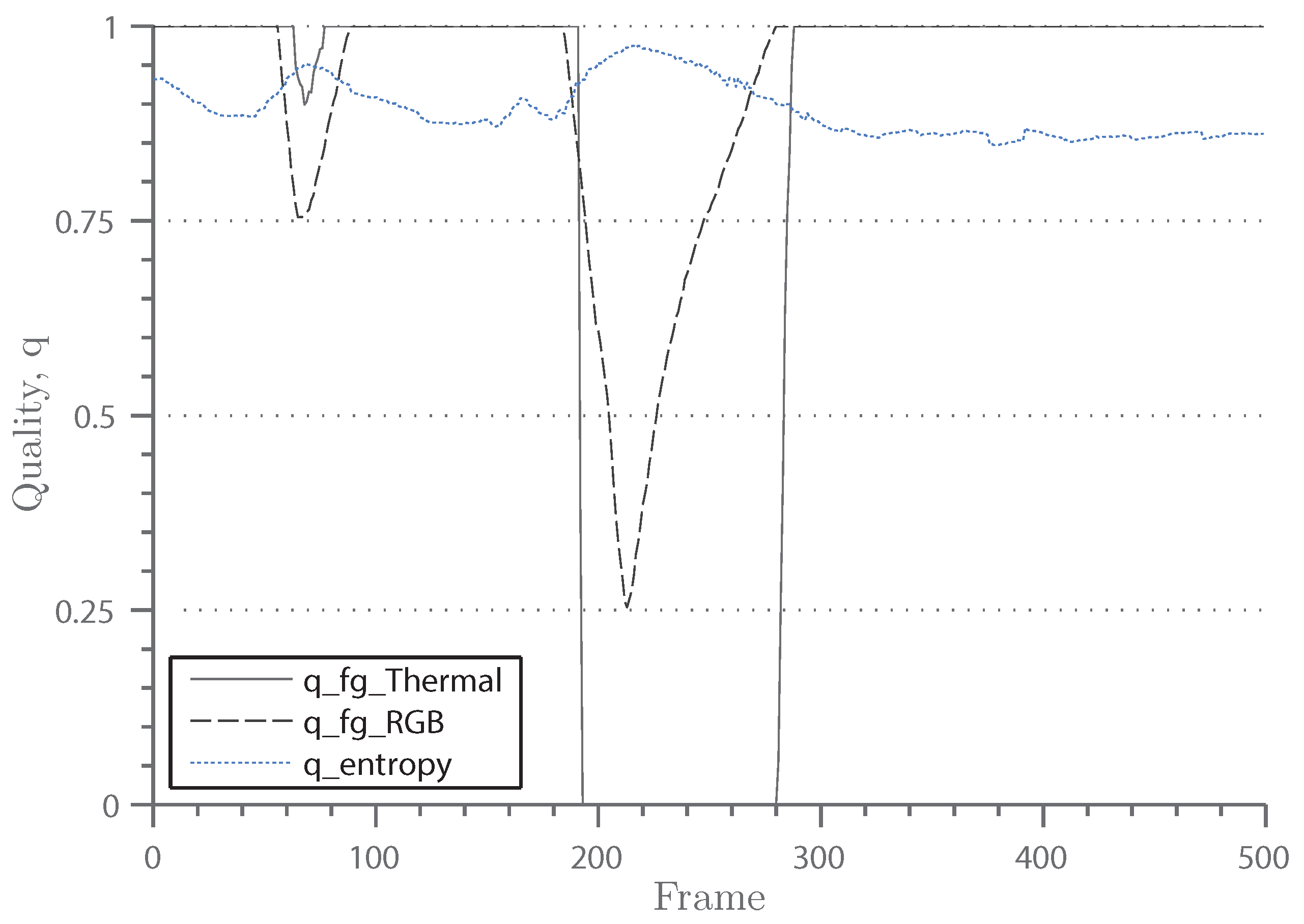
7.4.1. Context Awareness
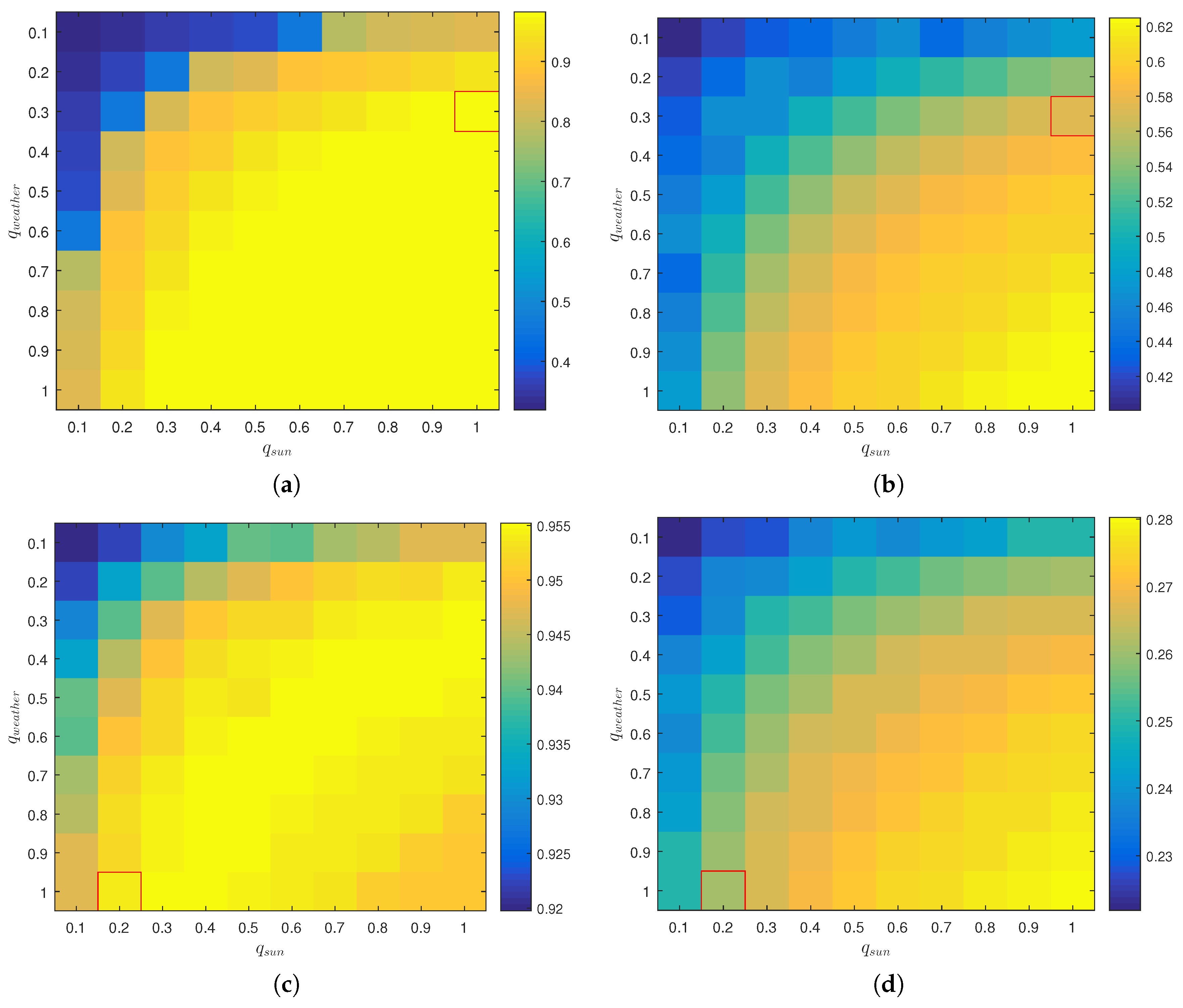
7.4.2. Parameter Sensitivity
7.4.3. Automatic Gain Control
7.4.4. Changing Illumination
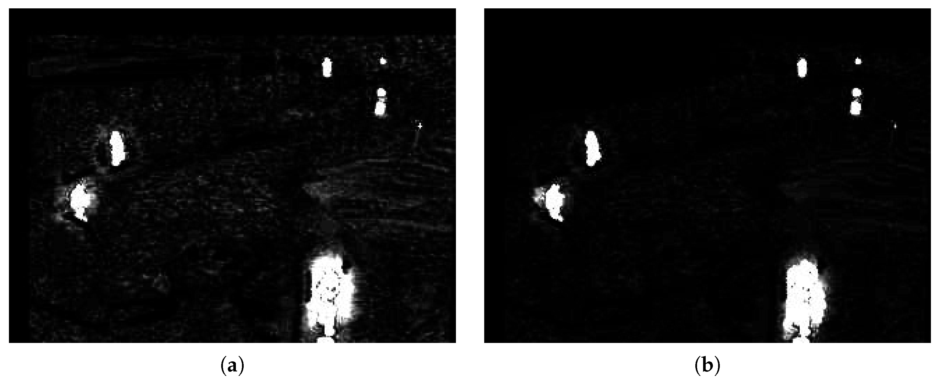
7.4.5. Artifact Reduction
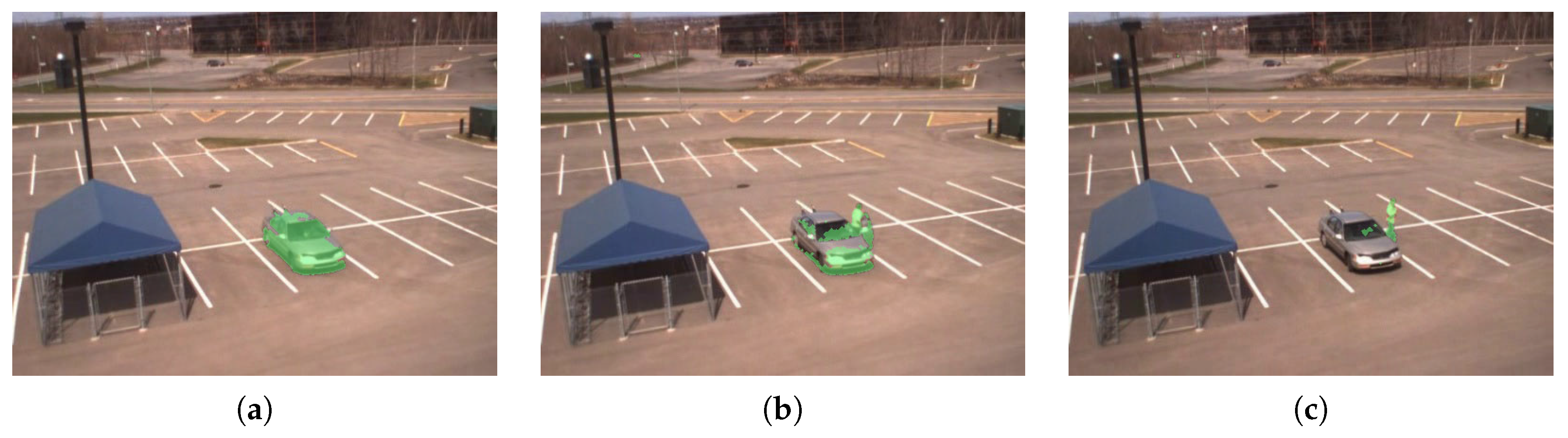
7.4.6. Long-Staying Objects
8. Conclusions and Future Perspectives
Acknowledgments
Author Contributions
Conflicts of Interest
References
- Kastrinaki, V.; Zervakis, M.; Kalaitzakis, K. A survey of video processing techniques for traffic applications. Image Vis. Comput. 2003, 21, 359–381. [Google Scholar] [CrossRef]
- Buch, N.; Velastin, S.A.; Orwell, J. A review of computer vision techniques for the analysis of urban traffic. IEEE Trans. Intell. Transp. Syst. 2011, 12, 920–939. [Google Scholar] [CrossRef]
- Chen, T.H.; Chen, J.L.; Chen, C.H.; Chang, C.M. Vehicle detection and counting by using headlight information in the dark environment. In Proceedings of the Third International Conference on Intelligent Information Hiding and Multimedia Signal Processing (IIHMSP 2007), Kaohsiung City, Taiwan, 26–28 November 2007; pp. 519–522.
- Robert, K. Night-time traffic surveillance: A robust framework for multi-vehicle detection, classification and tracking. In Proceedings of the Sixth IEEE International Conference on Advanced Video and Signal Based Surveillance (AVSS’09), Genova, Italy, 2–4 September 2009; pp. 1–6.
- Zou, Y.; Shi, G.; Shi, H.; Wang, Y. Image sequences based traffic incident detection for signaled intersections using HMM. In Proceedings of the Ninth International Conference on Hybrid Intelligent Systems (HIS’09), Shenyang, China, 12–14 August 2009; pp. 257–261.
- Nieto, M.; Unzueta, L.; Barandiaran, J.; Cortés, A.; Otaegui, O.; Sánchez, P. Vehicle tracking and classification in challenging scenarios via slice sampling. EURASIP J. Adv. Signal Proc. 2011, 2011, 1–17. [Google Scholar] [CrossRef]
- Zou, Q.; Ling, H.; Luo, S.; Huang, Y.; Tian, M. Robust nighttime vehicle detection by tracking and grouping headlights. IEEE Trans. Intell. Transp. Syst. 2015, 16, 2838–2849. [Google Scholar] [CrossRef]
- Strigel, E.; Meissner, D.; Dietmayer, K. Vehicle detection and tracking at intersections by fusing multiple camera views. In Proceedings of the 2013 IEEE Intelligent Vehicles Symposium (IV), Gold Coast, Australia, 23–26 June 2013; pp. 882–887.
- Gade, R.; Moeslund, T.B. Thermal cameras and applications: A survey. Mach. Vis. Appl. 2014, 25, 245–262. [Google Scholar] [CrossRef]
- Hall, D.; Llinas, J. Multisensor Data Fusion; CRC Press: Boca Raton, FL, USA, 2001. [Google Scholar]
- Serrano-Cuerda, J.; Fernández-Caballero, A.; López, M.T. Selection of a visible-light vs. thermal infrared sensor in dynamic environments based on confidence measures. Appl. Sci. 2014, 4, 331–350. [Google Scholar] [CrossRef]
- Kwon, H.; Der, S.Z.; Nasrabadi, N.M. Adaptive multisensor target detection using feature-based fusion. Opt. Eng. 2002, 41, 69–80. [Google Scholar] [CrossRef]
- Conaire, C.O.; O’Connor, N.E.; Cooke, E.; Smeaton, A.F. Comparison of fusion methods for thermo-visual surveillance tracking. In Proceedings of the 9th International Conference on Information Fusion, Florence, Italy, 10–13 July 2006; pp. 1–7.
- Heather, J.P.; Smith, M.I. Multimodal image registration with applications to image fusion. In Proceedings of the 8th International Conference on Information Fusion, Philadelphia, PA, USA, 25–28 July 2005; pp. 372–379.
- Hrkać, T.; Kalafatić, Z.; Krapac, J. Infrared-Visual Image Registration Based on Corners and Hausdorff Distance. In Image Analysis; Springer: Berlin/Heidelberg, Germany, 2007; pp. 383–392. [Google Scholar]
- Istenic, R.; Heric, D.; Ribaric, S.; Zazula, D. Thermal and visual image registration in Hough parameter space. In Proceedings of the 2007 14th International Workshop on Systems, Signals and Image Processing, and the 6th EURASIP Conference Focused on Speech and Image Processing, Multimedia Communications and Services, Maribor, Slovenia, 27–30 June 2007; pp. 106–109.
- Shah, P.; Merchant, S.; Desai, U.B. Fusion of surveillance images in infrared and visible band using curvelet, wavelet and wavelet packet transform. Int. J. Wavelets Multiresolut. Inf. Proc. 2010, 8, 271–292. [Google Scholar] [CrossRef]
- Chen, S.; Leung, H. An EM-CI based approach to fusion of IR and visual images. In Proceedings of the 12th International Conference on Information Fusion (FUSION’09), Seattle, WA, USA, 6–9 July 2009; pp. 1325–1330.
- Lallier, E.; Farooq, M. A real time pixel-level based image fusion via adaptive weight averaging. In Proceedings of the Third International Conference on Information Fusion (FUSION 2000), Paris, France, 10–13 July 2000.
- St-Laurent, L.; Maldague, X.; Prévost, D. Combination of colour and thermal sensors for enhanced object detection. In Proceedings of the 2007 10th International Conference on Information Fusion, Quebec City, QC, Canada, 9–12 July 2007; pp. 1–8.
- Vollmer, M.; Möllmann, K.P. Infrared Thermal Imaging: Fundamentals, Research and Applications; John Wiley & Sons: New York, NY, USA, 2010. [Google Scholar]
- Prati, A.; Mikic, I.; Trivedi, M.M.; Cucchiara, R. Detecting moving shadows: Algorithms and evaluation. IEEE Trans. Pattern Anal. Mach. Intell. 2003, 25, 918–923. [Google Scholar] [CrossRef]
- Michalsky, J.J. The astronomical almanac’s algorithm for approximate solar position (1950–2050). Sol. Energy 1988, 40, 227–235. [Google Scholar] [CrossRef]
- Ridpath, I. A Dictionary of Astronomy, 2nd ed.; Oxford University Press: Oxford, UK, 2012. [Google Scholar]
- National Oceanic and Atmospheric Administration’s National Weather Service. Weather Element List and Suggested Icons. Avilable online: http://w1.weather.gov/xml/currentobs/weather.php (accessed on 28 September 2016).
- Garg, K.; Nayar, S.K. Vision and rain. Int. J. Comput. Vis. 2007, 75, 3–27. [Google Scholar] [CrossRef]
- Hartley, R.; Zisserman, A. Multiple View Geometry in Computer Vision; Cambridge University Press: Cambridge, UK, 2003. [Google Scholar]
- Stauffer, C.; Grimson, W.E.L. Adaptive background mixture models for real-time tracking. In Proceedings of the IEEE Computer Society Conference on Computer Vision and Pattern Recognition, Fort Collins, CO, USA, 23–25 June 1999.
- Yao, L.; Ling, M. An Improved Mixture-of-Gaussians Background Model with Frame Difference and Blob Tracking in Video Stream. Sci. World J. 2014, 2014, 424050. [Google Scholar] [CrossRef] [PubMed]
- Alemán-Flores, M.; Alvarez, L.; Gomez, L.; Santana-Cedrés, D. Line detection in images showing significant lens distortion and application to distortion correction. Pattern Recognit. Lett. 2014, 36, 261–271. [Google Scholar] [CrossRef]
- Davis, J.W.; Sharma, V. Background-subtraction using contour-based fusion of thermal and visible imagery. Comput. Vis. Image Underst. 2007, 106, 162–182. [Google Scholar] [CrossRef]
- Kim, K.; Chalidabhongse, T.H.; Harwood, D.; Davis, L. Real-time foreground–background segmentation using codebook model. Real Time Imaging 2005, 11, 172–185. [Google Scholar] [CrossRef]
- Zivkovic, Z. Improved adaptive Gaussian mixture model for background subtraction. In Proceedings of the 17th International Conference on IEEE Pattern Recognition, 2004 (ICPR 2004), Cambridge, UK, 26–26 August 2004; pp. 28–31.


| Weather Condition [25] | Category | |
|---|---|---|
| Clear | Good conditions | 1.0 |
| Overcast | Low/varying illumination | 0.8 |
| Cloudy | ||
| Light mist, drizzle | ||
| Heavy drizzle, mist | Reflections/moisture | 0.6 |
| Light rain | ||
| Snow | Particle occlusion/precipitation | 0.3 |
| Hail | ||
| Heavy rain | ||
| Thunderstorm | ||
| Fog, haze | Reduced visibility | 0.3 |
| Dust, sand, smoke |
 | ||||
| Day | Night | Auto Gain | Heavy Rain | Snowing |
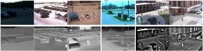 | |||||
| INO ParkingEvening | INO ParkingSnow | INO CoatDeposit | INO TreesAndRunner | OTCBVS 3 | OTCBVS 4 |
| Sequence | Annotated Frames | Average Number of Objects per Frame | Weather Classification | Sun Altitude | |||
|---|---|---|---|---|---|---|---|
| Day | 70 | 6.4 | Good conditions | 1.0 | 1.0 | 0.95 | |
| Night | 70 | 6.9 | Low illumination | 0.8 | 0.20 | 1.0 | |
| Auto Gain | 180 | 9.0 | Moisture | 0.6 | 1.0 | 1.0 | |
| Heavy Rain | 70 | 6.7 | Moisture | 0.6 | 1.0 | 1.0 | |
| Snowing | 70 | 5.6 | Precipitation | 0.3 | 1.0 | 1.0 | |
| INO ParkingEvening | 70 | 2.1 | Good conditions | 1.0 | 0.20 | 1.0 | |
| INO ParkingSnow | 70 | 7.0 | Low illumination | 0.8 | 1.0 | 1.0 | |
| INO CoatDeposit | 70 | 2.8 | Low illumination | 0.8 | 1.0 | 0.98 | |
| INO TreesAndRunner | 70 | 1.0 | Low illumination | 0.8 | 0.50 | 0.30 | |
| OTCBVS 3 | 70 | 3.9 | Low illumination | 0.8 | 1.0 | 0.91 | |
| OTCBVS 4 | 70 | 1.0 | Good conditions | 1.0 | 1.0 | 1.0 |
| Parameter | Value | Description |
|---|---|---|
| α | GMM update rate | |
| K | 5 | Number of components for GMM |
| λ | 4 | Number of standard deviations for background acceptance for GMM |
| T | 1 | Segmentation threshold of the distance map |
| Background update rate for blob-based prediction | ||
| Foreground update rate for blob-based prediction | ||
| τ | Foreground ratio | |
| γ | 5.0 | Foreground deviation weight |
| ρ | 17 | Blob match radius (px) |
| Distance scaling factor for shadow regions | ||
| Distance scaling factor for predicted regions | ||
| Distance scaling factor for neutral regions | ||
| 0.2 | Minimum quality of | |
| 0.3 | Minimum quality of |
| Proposed | RGB | Thermal | RGBT | Select | |
|---|---|---|---|---|---|
| Day | 0.99 | 0.93 | 0.95 | 0.97 | 0.93 |
| 0.30 | 0.09 | 0.31 | 0.29 | 0.09 | |
| Night | 0.84 | 0.78 | 0.48 | 0.89 | 0.78 |
| 0.31 | 0.69 | 0.32 | 0.66 | 0.69 | |
| Auto Gain | 0.94 | 0.86 | 0.73 | 0.91 | 0.81 |
| 0.25 | 0.09 | 0.76 | 0.40 | 0.58 | |
| Heavy Rain | 0.92 | 0.46 | 0.69 | 0.48 | 0.69 |
| 0.22 | 0.26 | 0.11 | 0.27 | 0.11 | |
| Snowing | 0.96 | 0.79 | 0.21 | 0.92 | 0.21 |
| 0.52 | 0.52 | 0.25 | 0.55 | 0.25 | |
| INO ParkingEvening | 0.95 | 0.93 | 0.91 | 0.95 | 0.91 |
| 0.26 | 0.27 | 0.18 | 0.29 | 0.18 | |
| INO ParkingSnow | 0.98 | 0.86 | 0.99 | 0.96 | 0.99 |
| 0.32 | 0.78 | 0.40 | 0.35 | 0.40 | |
| INO CoatDeposit | 0.97 | 0.10 | 0.10 | 0.10 | 0.10 |
| 0.19 | 0.12 | 0.30 | 0.16 | 0.12 | |
| INO TreesAndRunner | 0.94 | 0.88 | 0.84 | 0.93 | 0.84 |
| 0.44 | 0.65 | 0.36 | 0.70 | 0.36 | |
| OTCBVS 3 | 0.95 | 0.75 | 0.94 | 0.90 | 0.78 |
| 0.56 | 0.96 | 0.74 | 0.96 | 0.93 | |
| OTCBVS 4 | 1.00 | 0.94 | 0.78 | 0.99 | 0.78 |
| 0.55 | 0.15 | 0.68 | 0.48 | 0.68 | |
| Average | 0.95 | 0.76 | 0.70 | 0.83 | 0.72 |
| 0.35 | 0.39 | 0.39 | 0.46 | 0.41 |
© 2016 by the authors; licensee MDPI, Basel, Switzerland. This article is an open access article distributed under the terms and conditions of the Creative Commons Attribution (CC-BY) license (http://creativecommons.org/licenses/by/4.0/).
Share and Cite
Alldieck, T.; Bahnsen, C.H.; Moeslund, T.B. Context-Aware Fusion of RGB and Thermal Imagery for Traffic Monitoring. Sensors 2016, 16, 1947. https://doi.org/10.3390/s16111947
Alldieck T, Bahnsen CH, Moeslund TB. Context-Aware Fusion of RGB and Thermal Imagery for Traffic Monitoring. Sensors. 2016; 16(11):1947. https://doi.org/10.3390/s16111947
Chicago/Turabian StyleAlldieck, Thiemo, Chris H. Bahnsen, and Thomas B. Moeslund. 2016. "Context-Aware Fusion of RGB and Thermal Imagery for Traffic Monitoring" Sensors 16, no. 11: 1947. https://doi.org/10.3390/s16111947