
Dicotyledon Weed Quantification Algorithm for Selective Herbicide Application in Maize Crops

 ,
,  , , , and
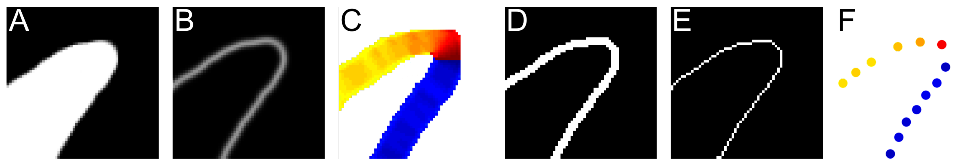
Abstract
:1. Introduction
1.1. Research in Weed Infestation
1.2. Sprayer Systems
1.3. Sensor Systems for Weed Detection
1.4. Plant/Weed Detection Systems
1.5. Contribution and Structure of This Work
2. Materials and Methods
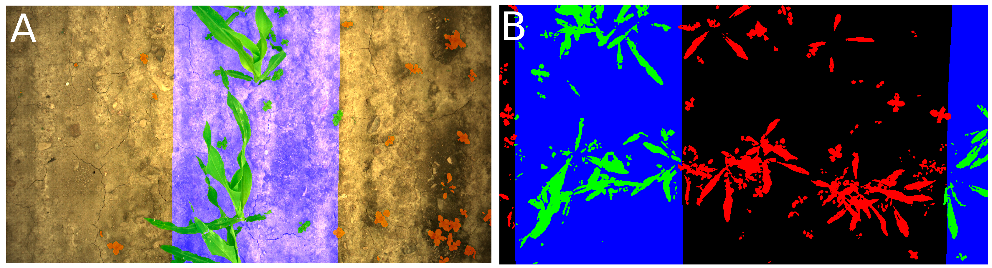
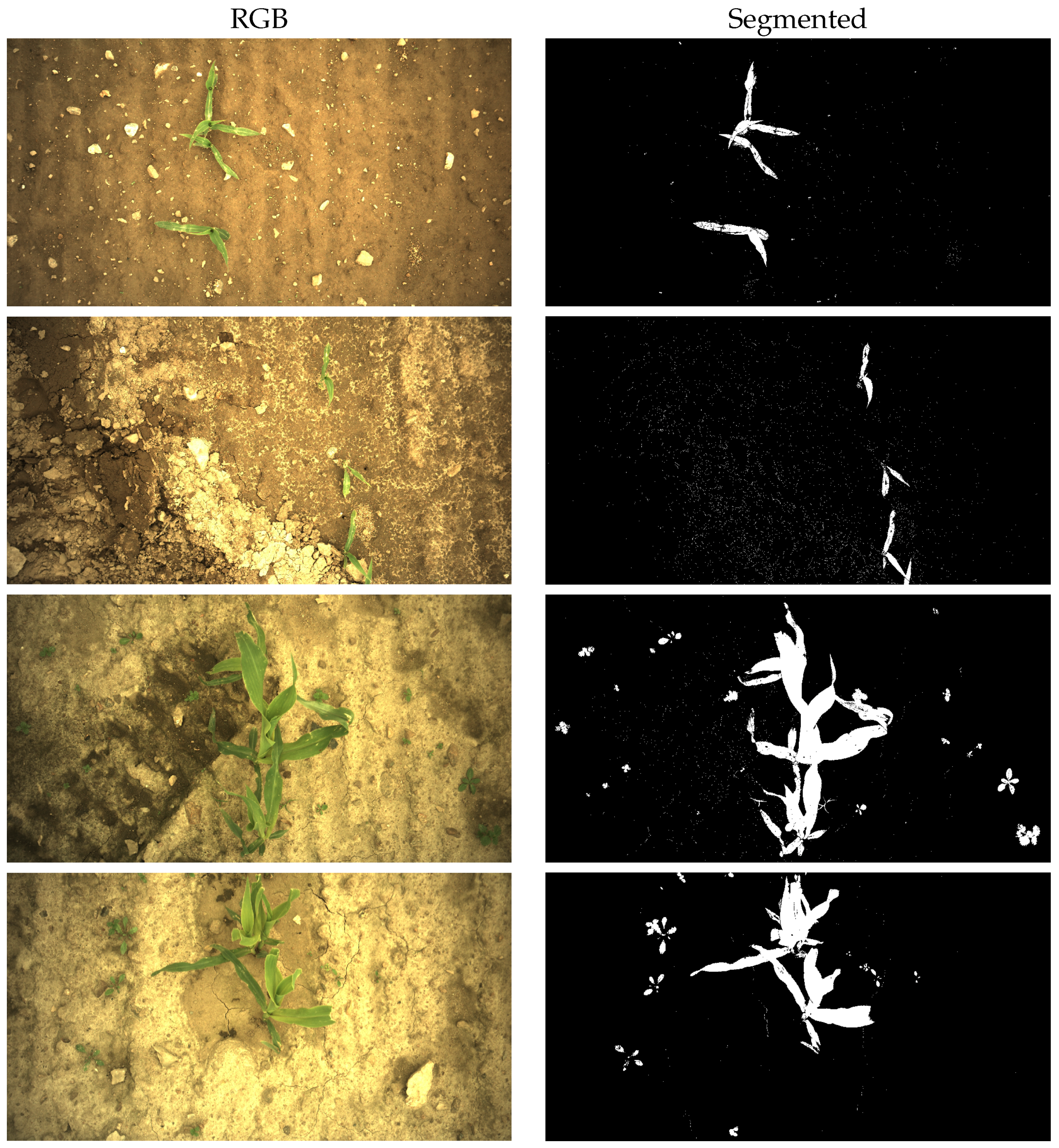
2.1. Image Acquisition and Segmentation
2.2. MoDiCoVi Dicotyledon Weed Quantifying Algorithm
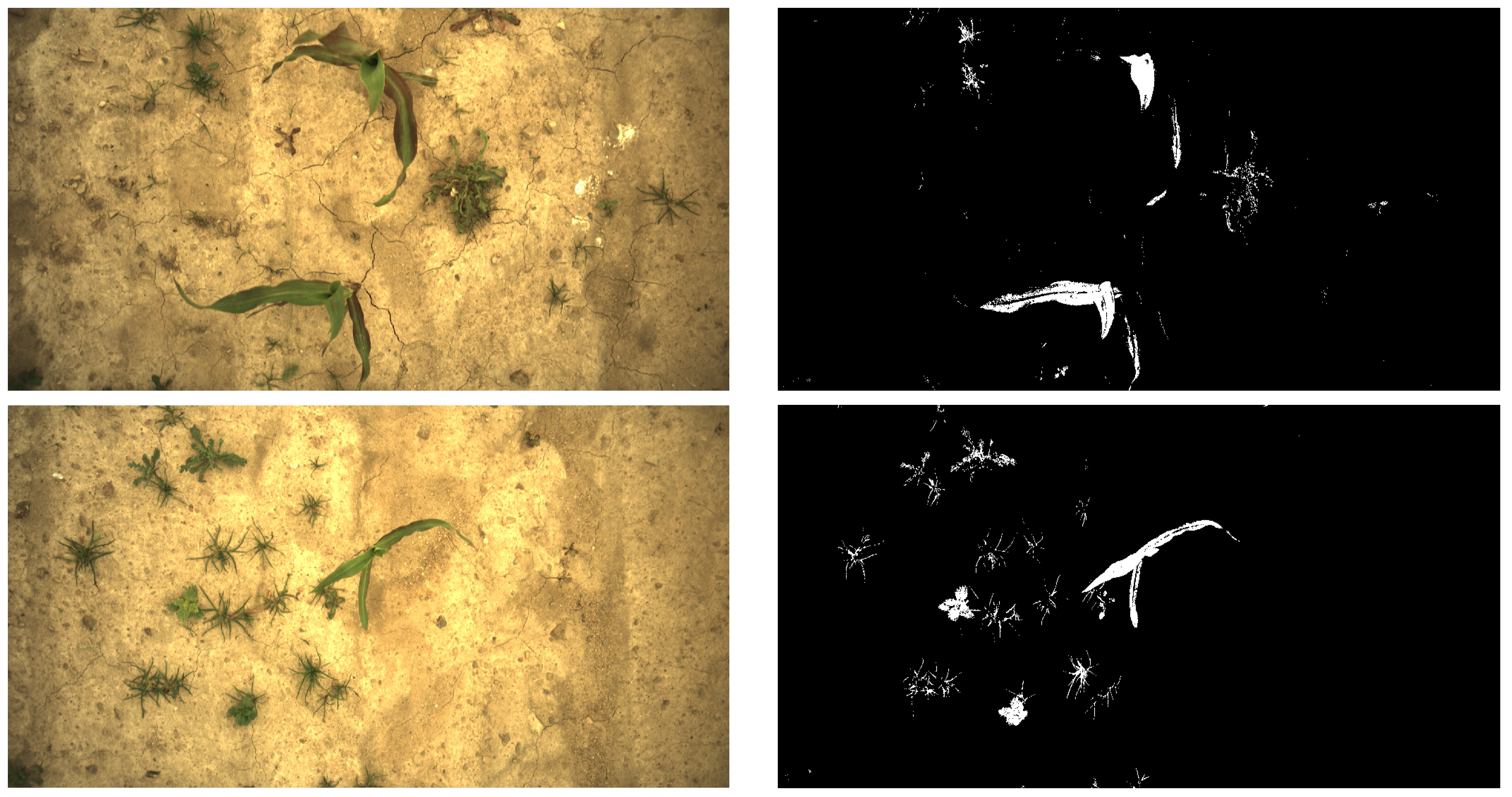
- The Bayer pattern is segmented into a binary vegetation/soil image.
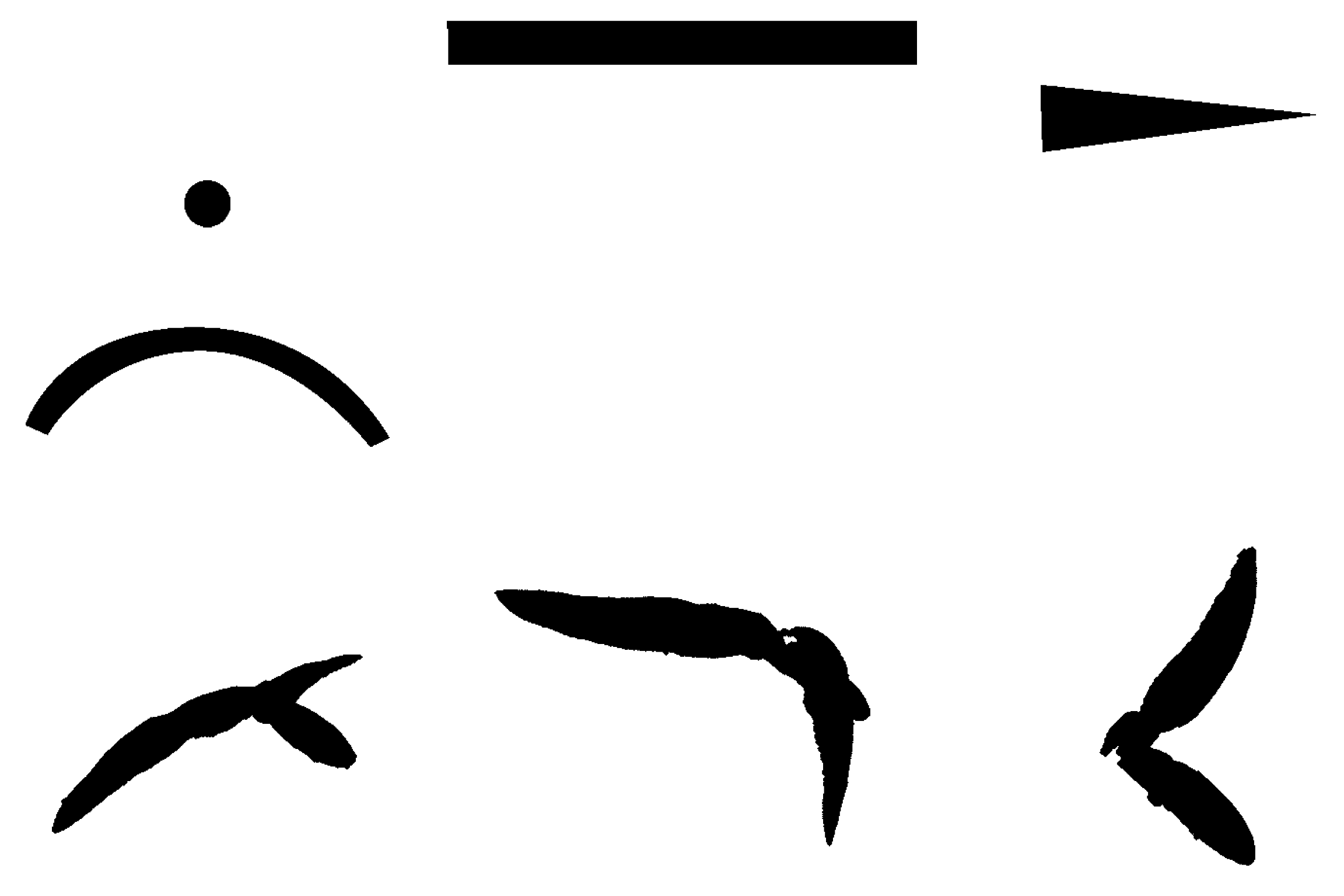
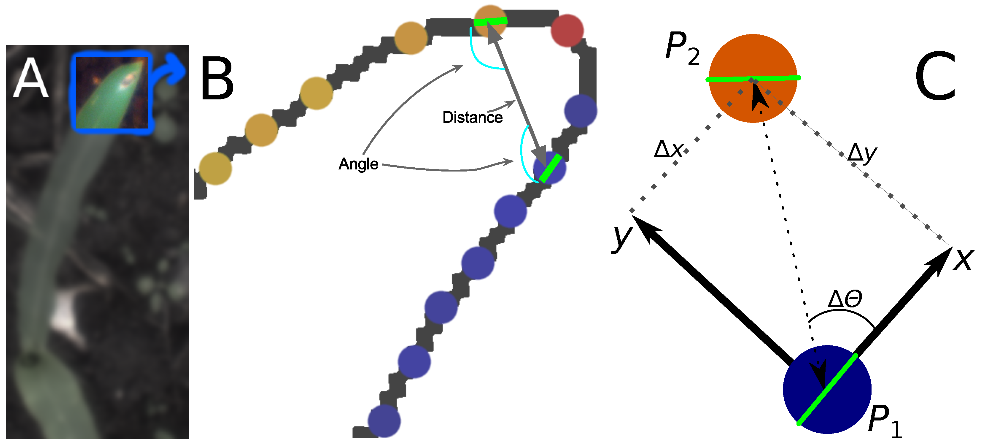
- Contours are located, and a subset of edge segments along the contours is chosen for further analysis.
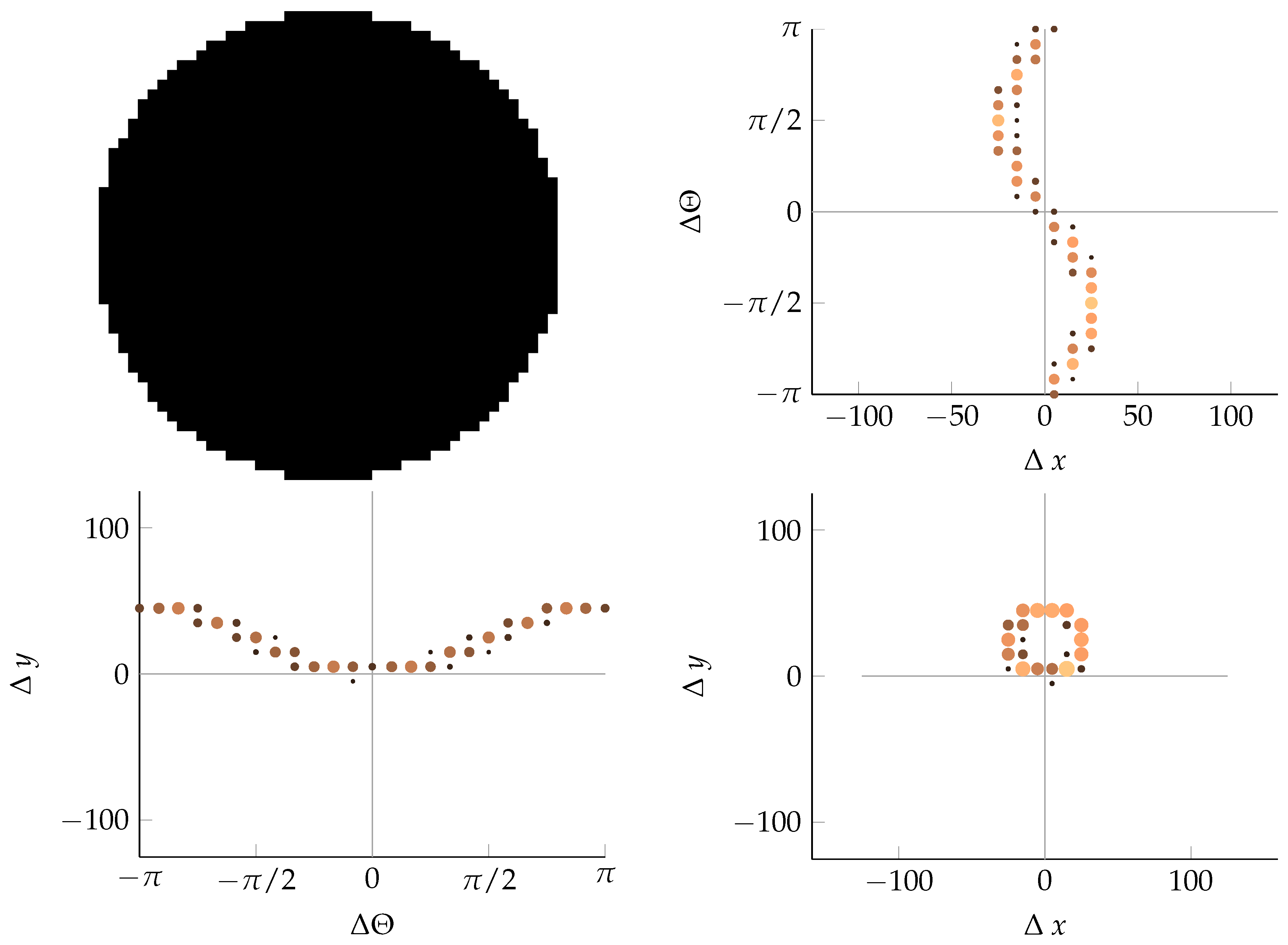
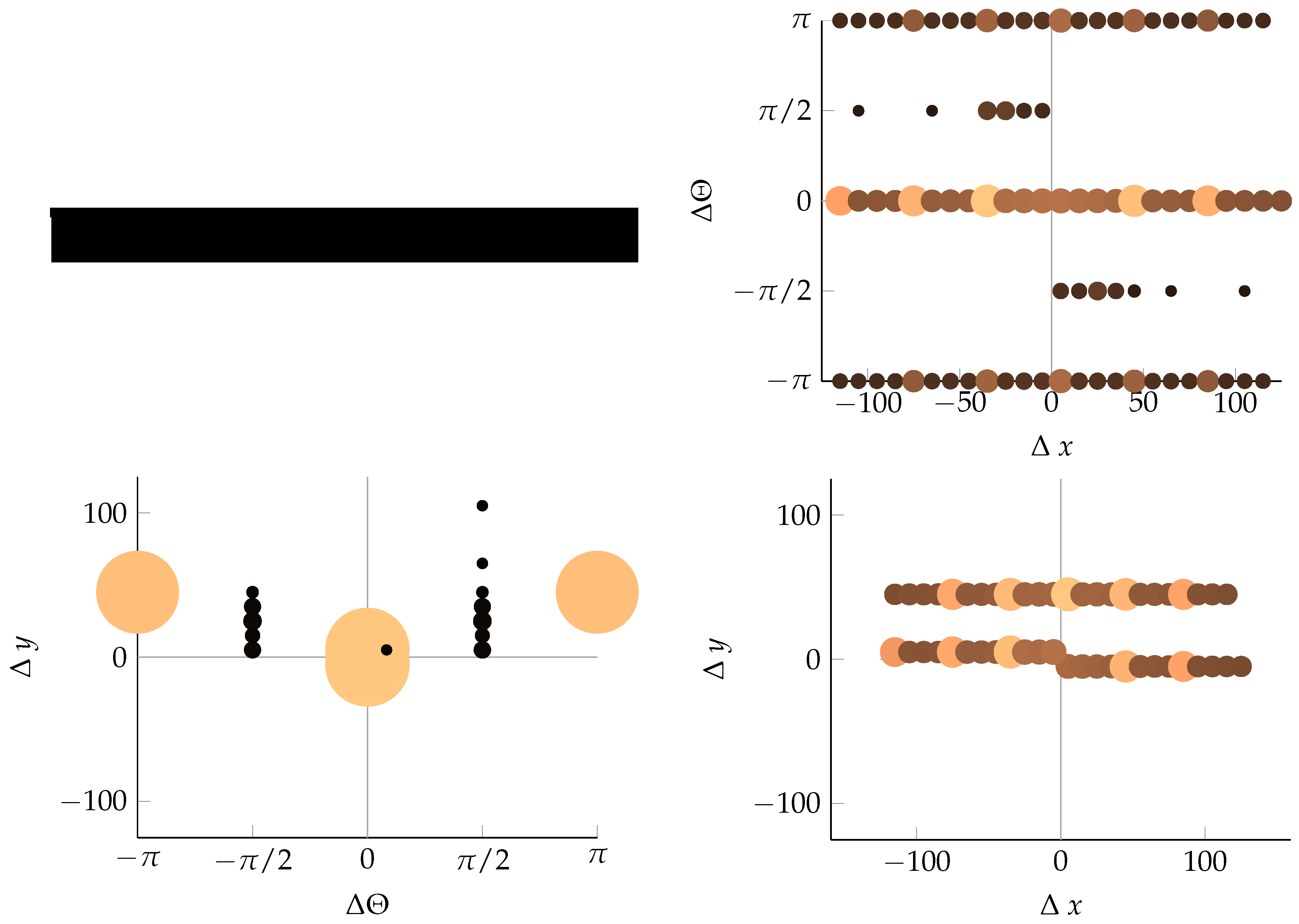
- The relative locations of nearby edge segments are calculated.
- The probability distribution of coordinates of the nearby edge segments is calculated. Using this information, the number of weed pixels in the image is estimated.
2.2.1. Find Directional Edges
2.2.2. Calculating Relative Coordinates of Edge Segments
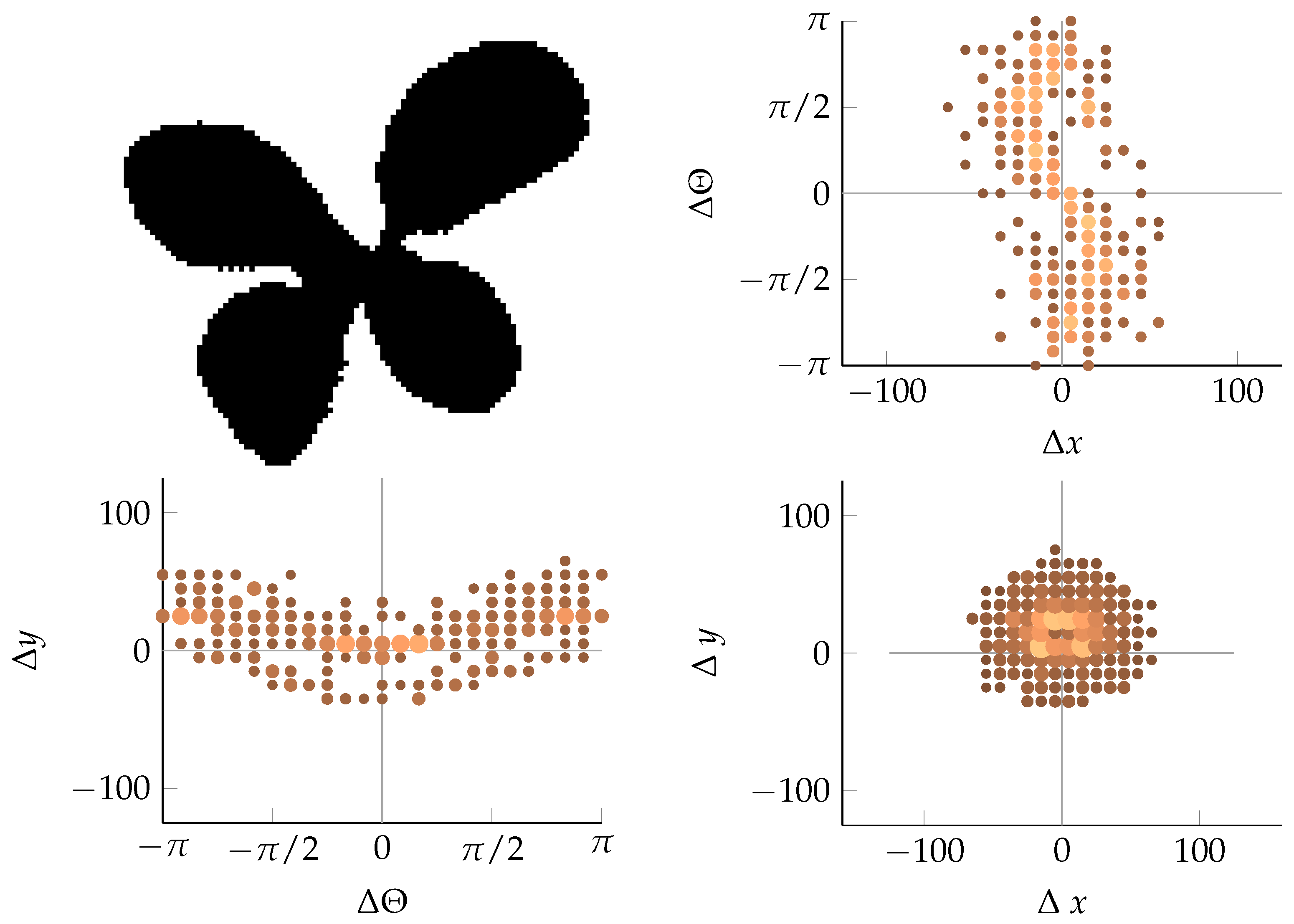
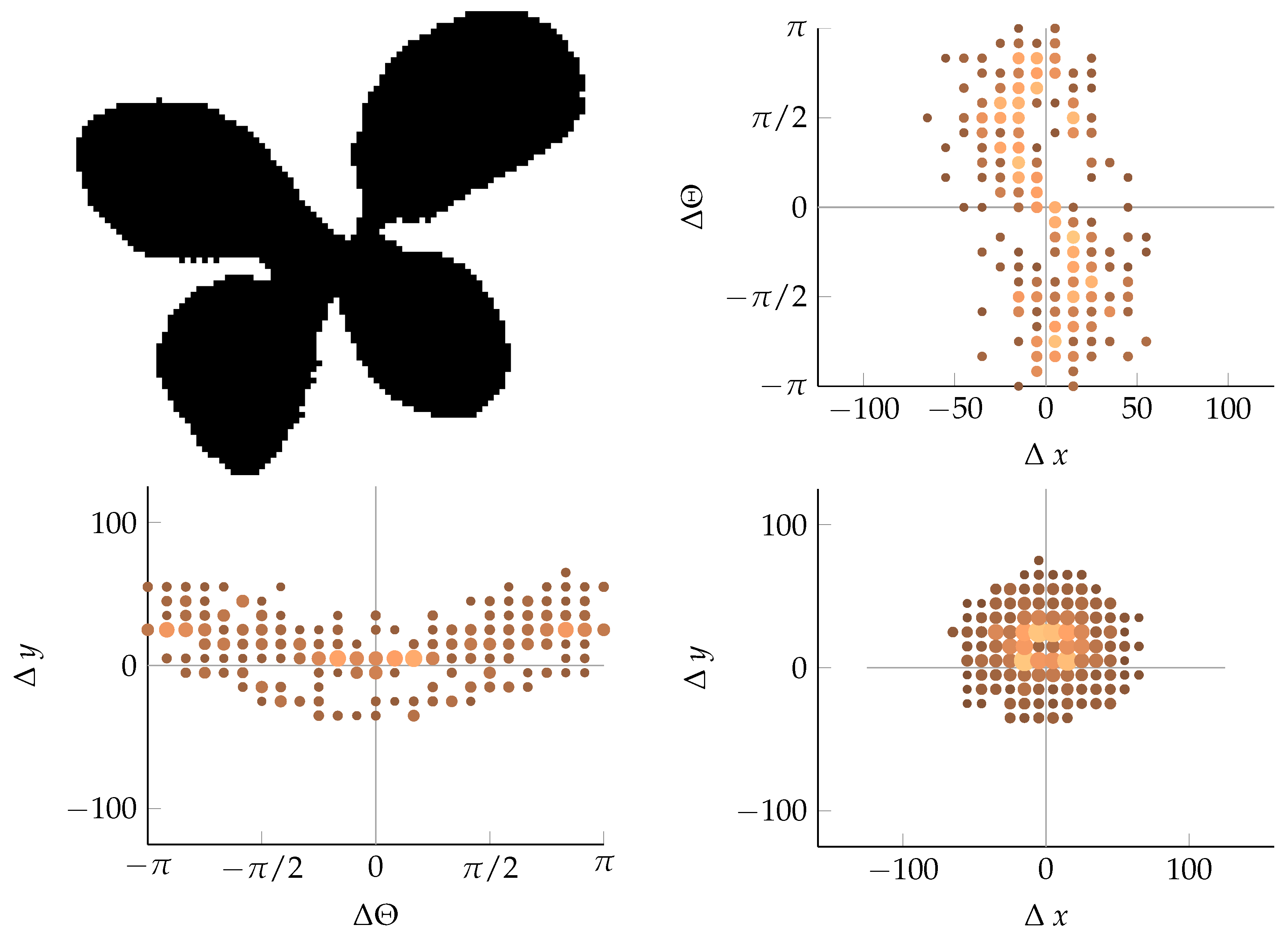
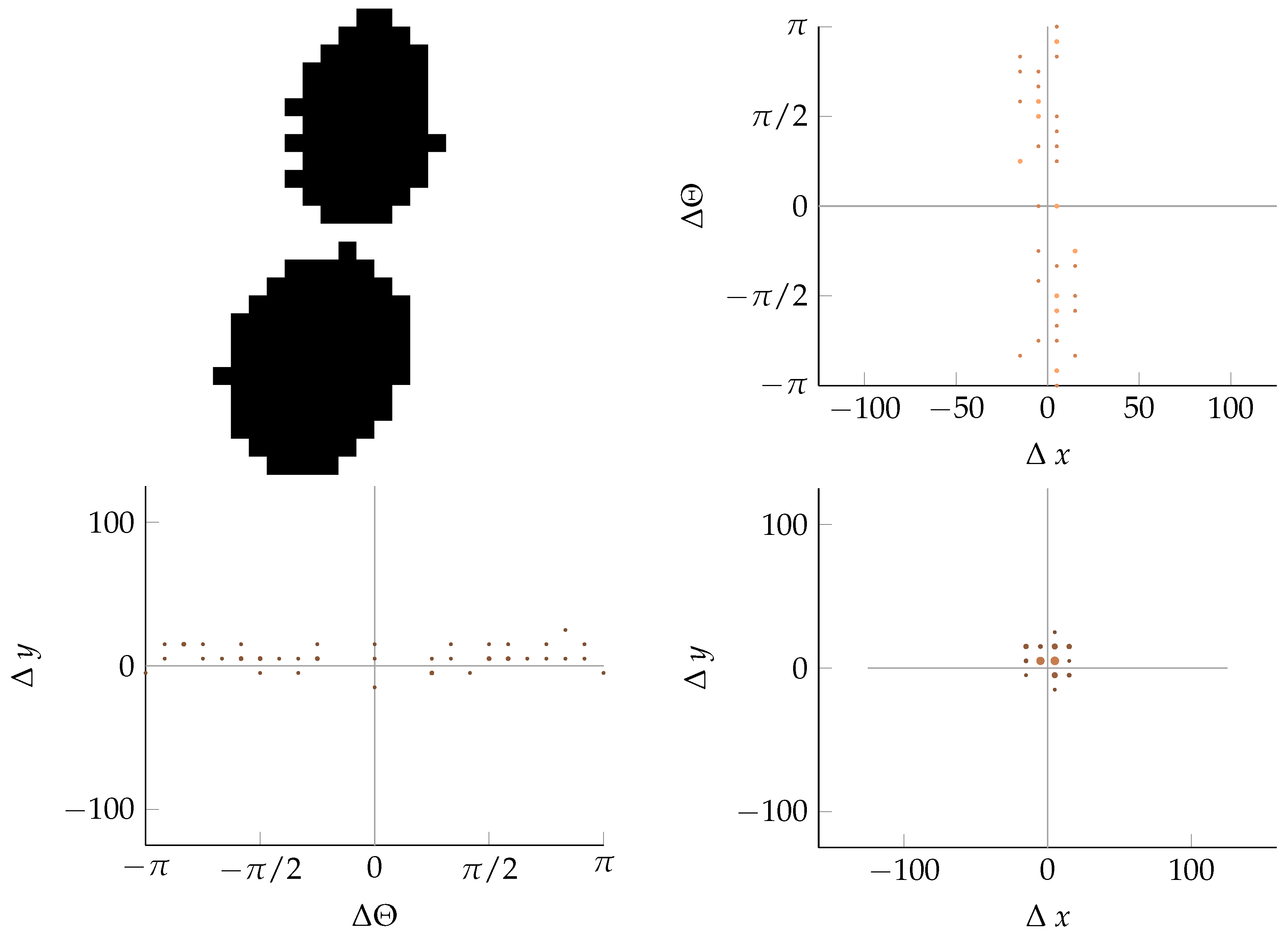
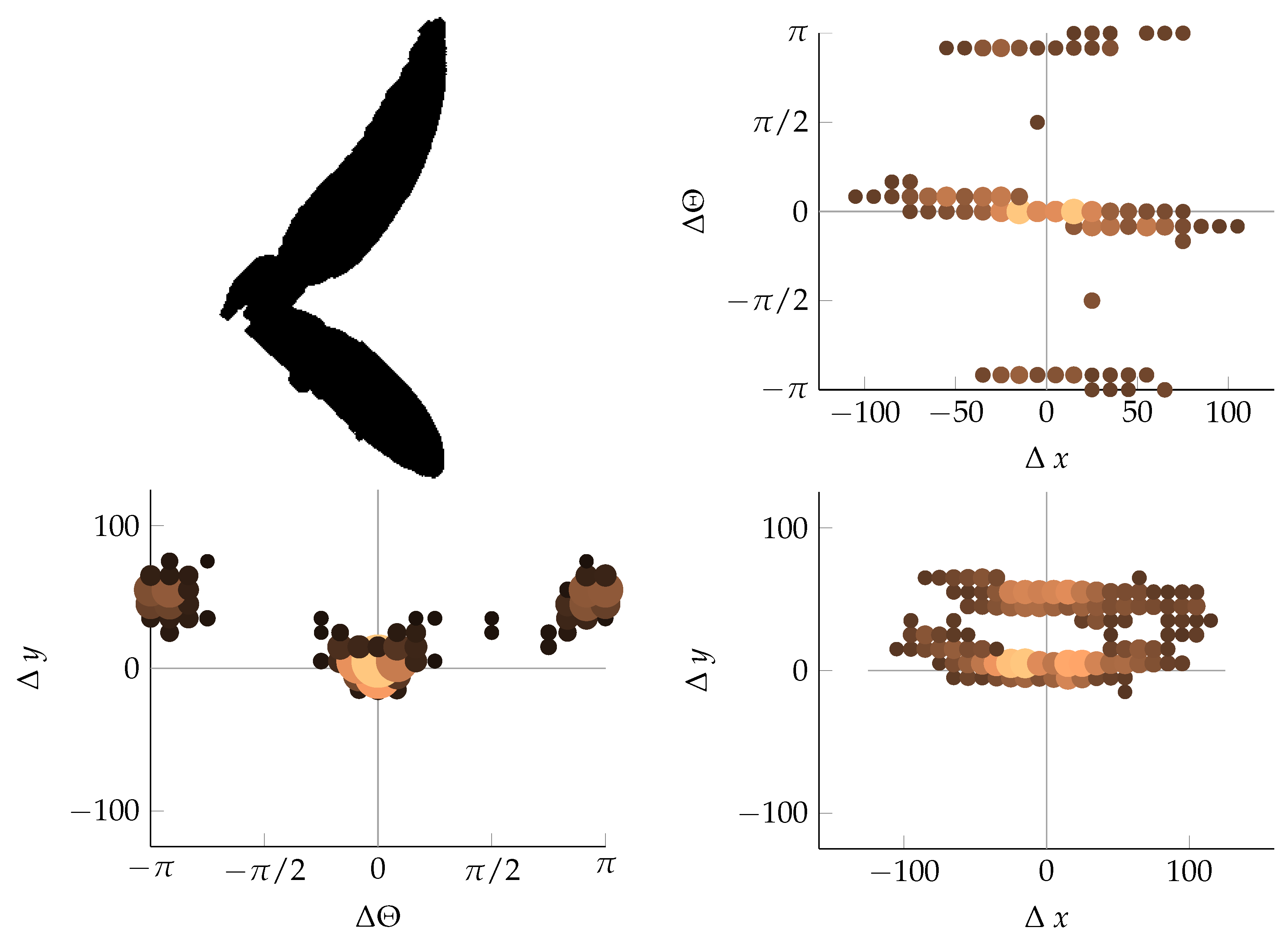
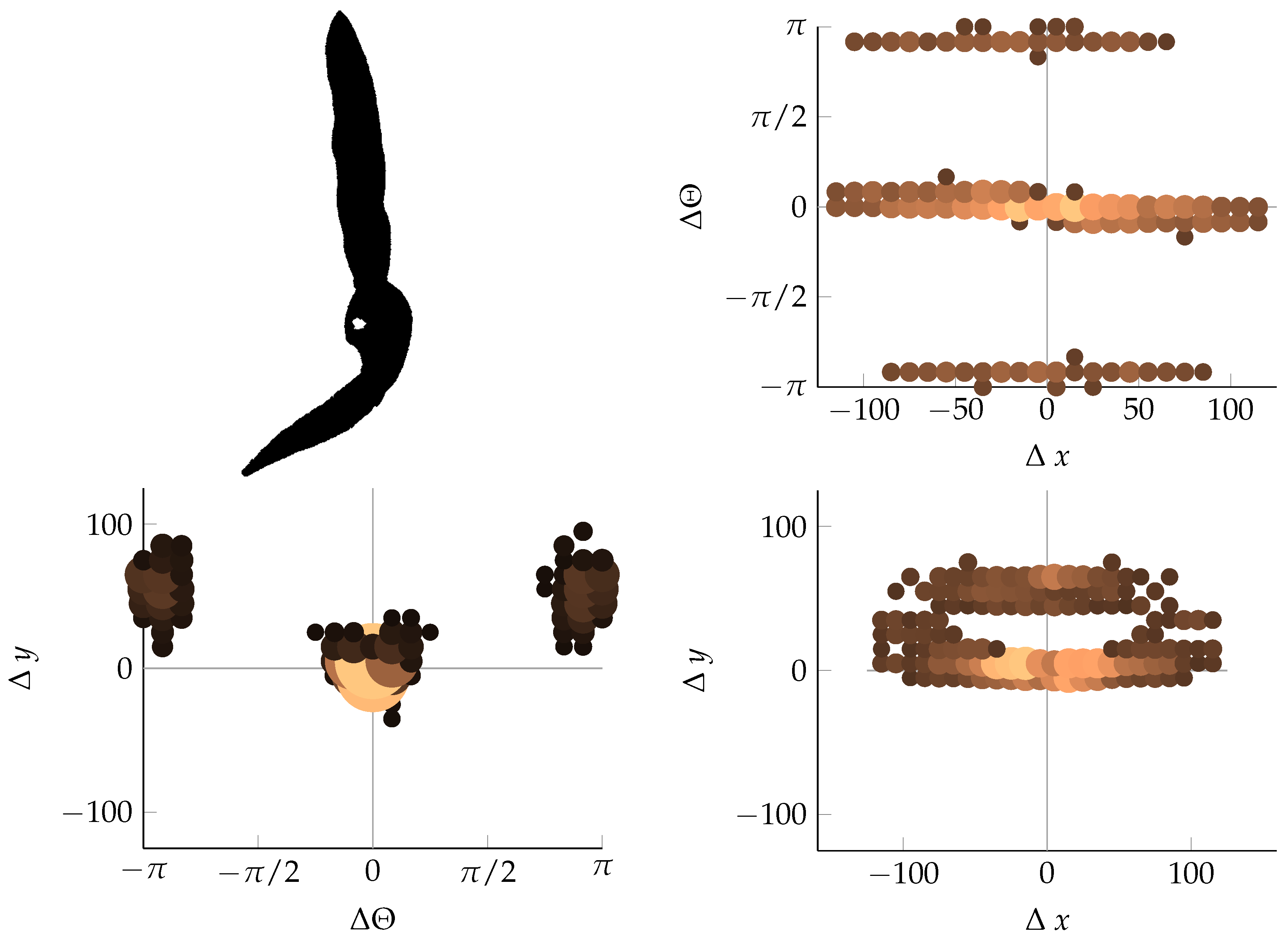
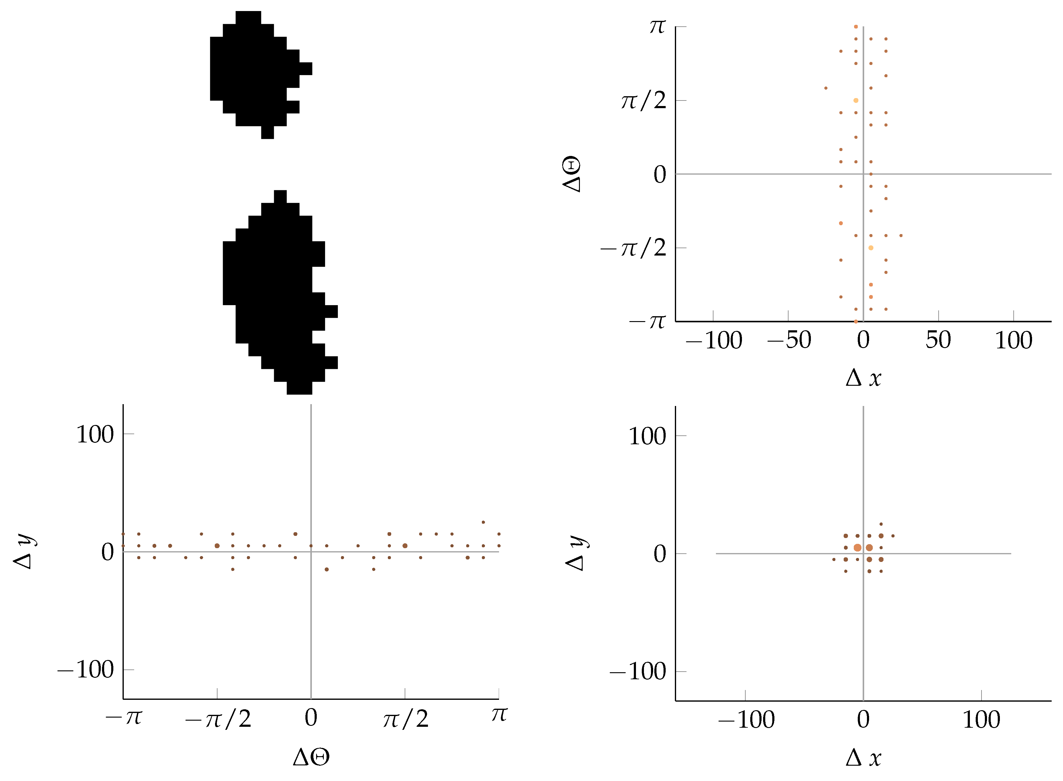
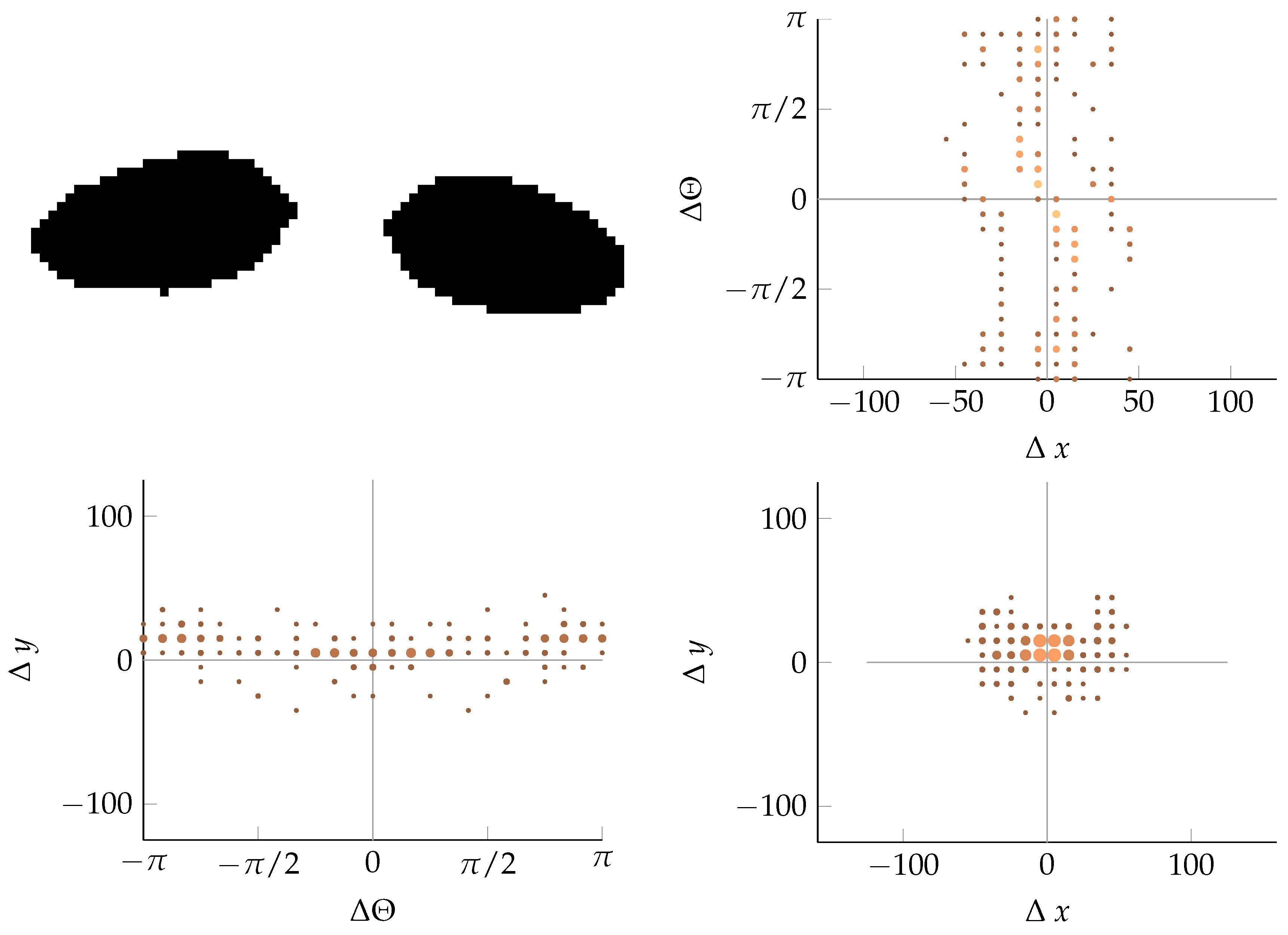
2.2.3. Coordinate Distribution Analysis
2.2.4. Adaptation to MoDiCoVi: Predicting the Amount of Weed Per Unit Area
2.2.5. Setting of Threshold Levels
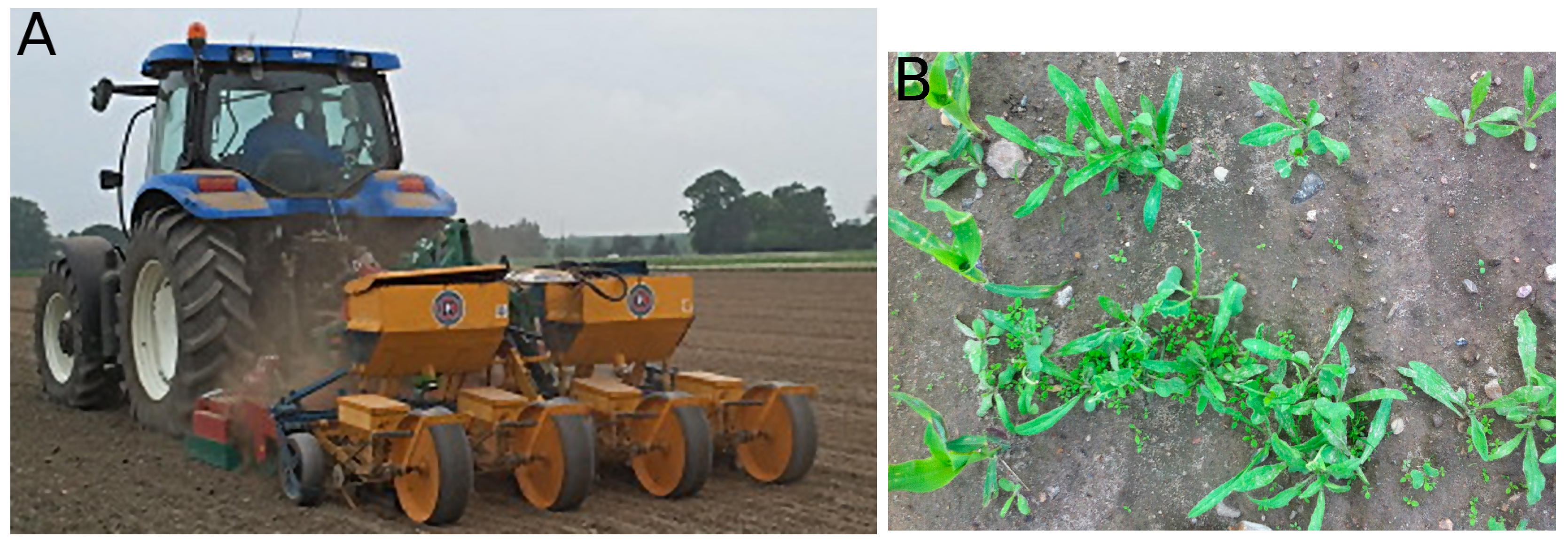
2.3. Evaluating the Experimental Layout
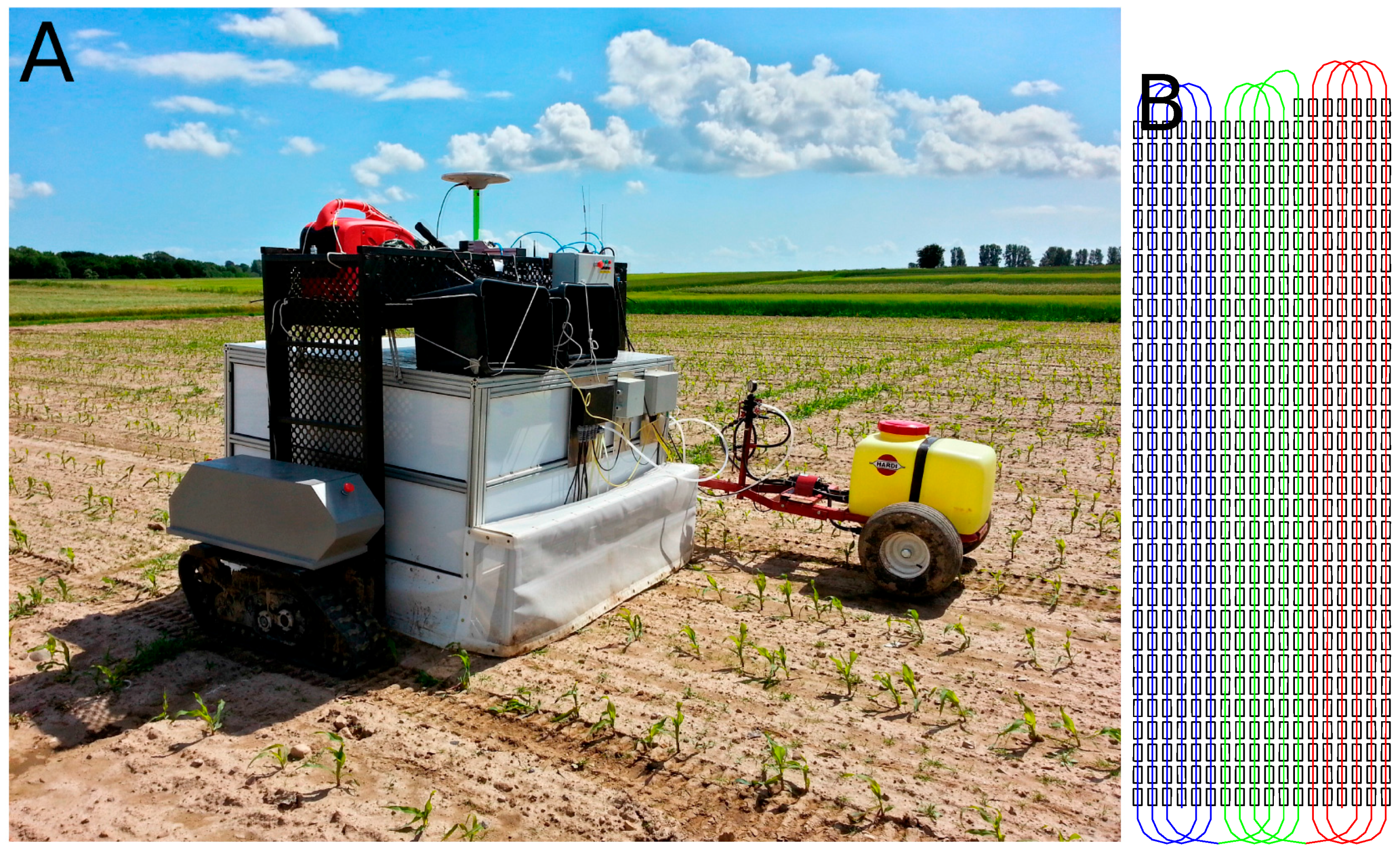
2.4. Automated Trial Execution
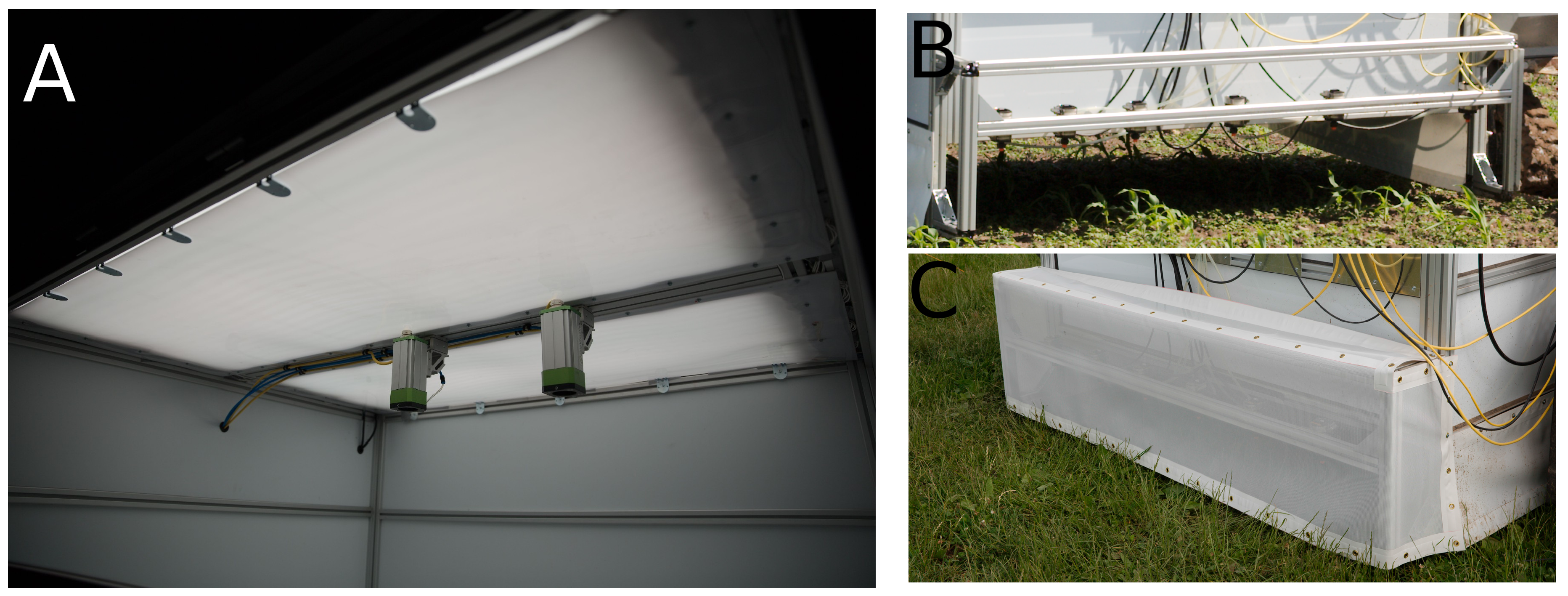
2.4.1. Automated Tool Carrier
2.4.2. Grid-Spraying Tool
2.4.3. Data Pre-Processing and Visualization
3. Results
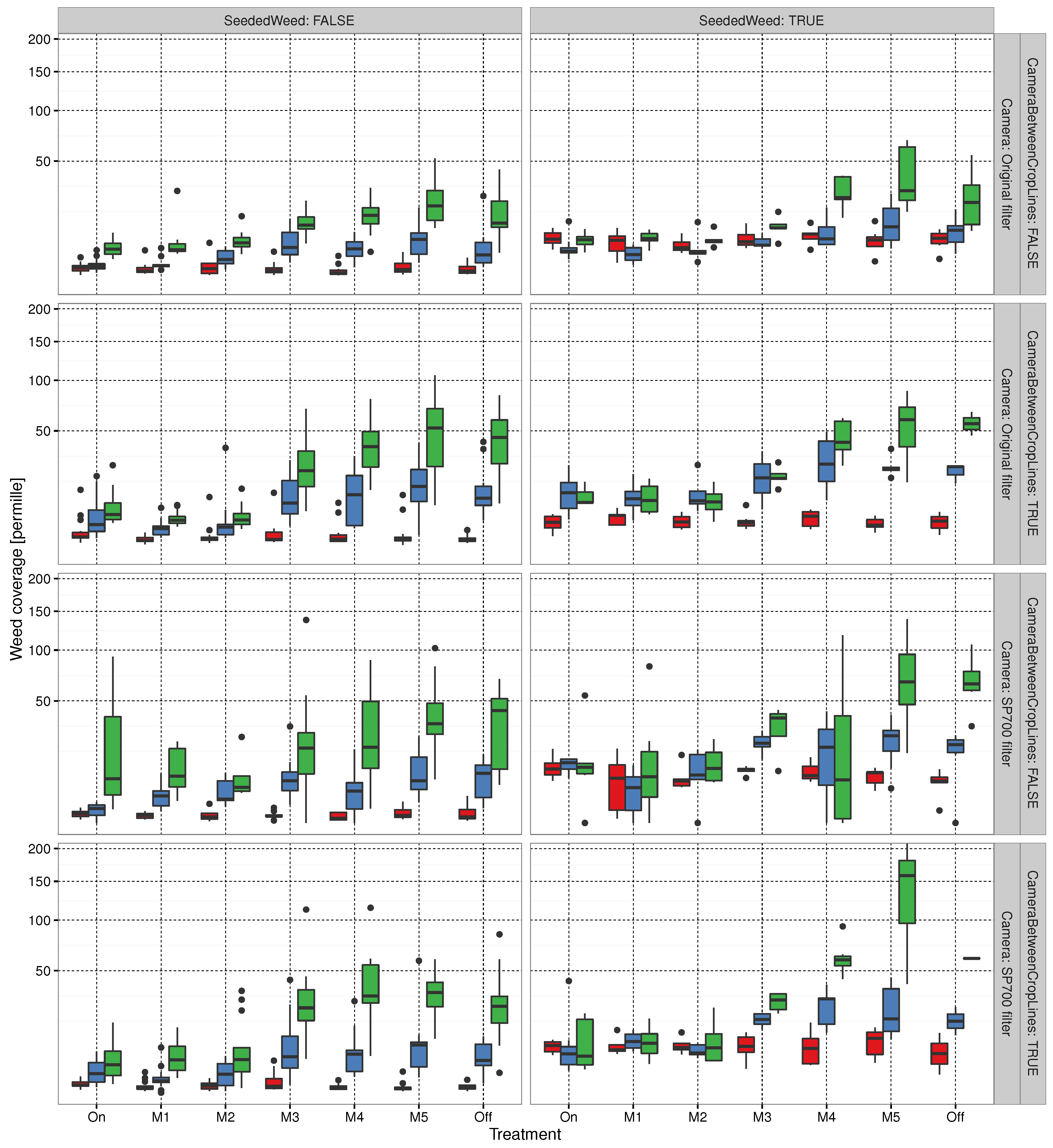
3.1. Evaluating Experimental Layout
3.2. Automated Trial Execution
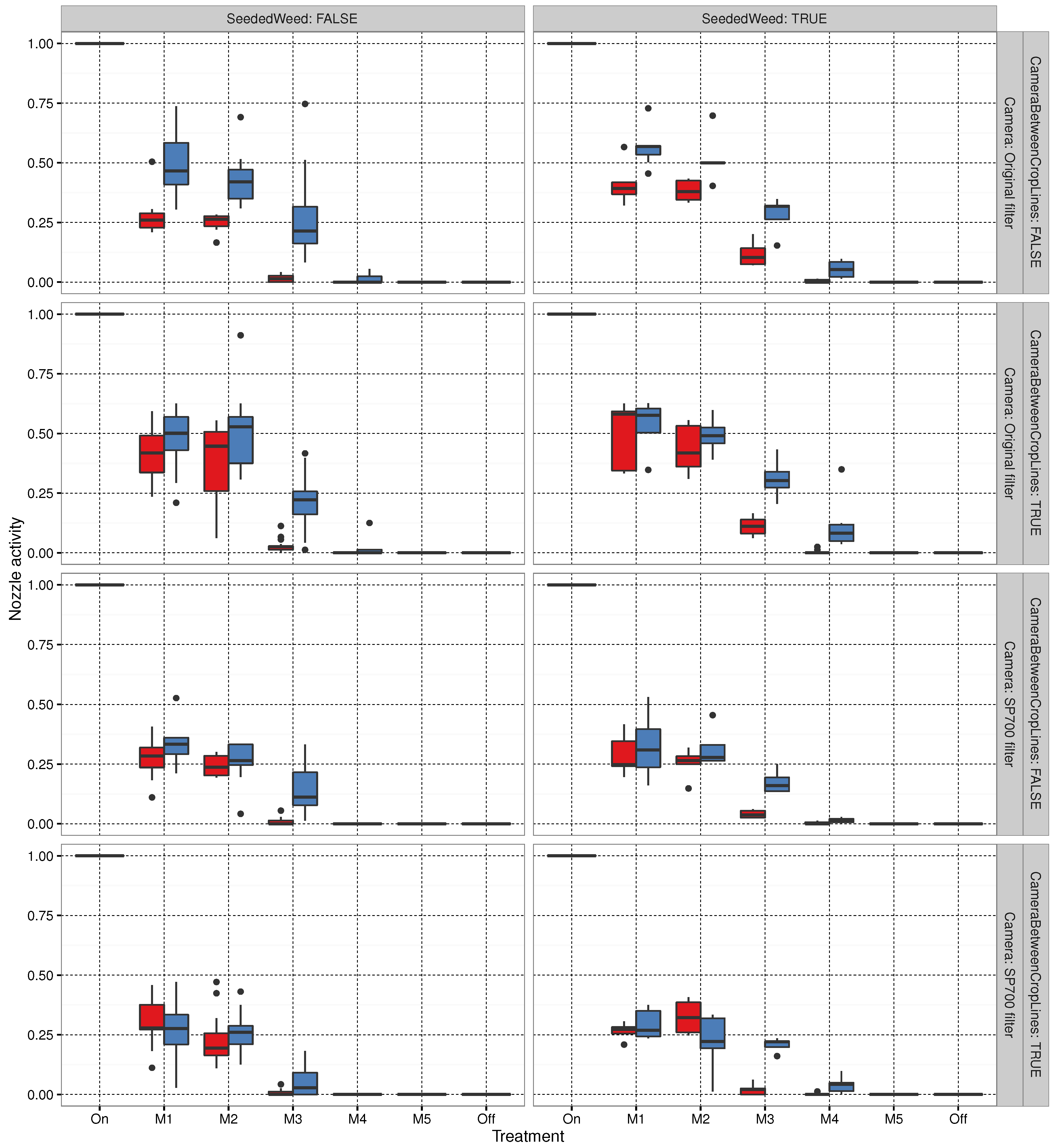
3.3. Sprayer Activity
4. Discussion
5. Conclusions
Acknowledgments
Author Contributions
Conflicts of Interest
Appendix A. Examples of Segmentation Results

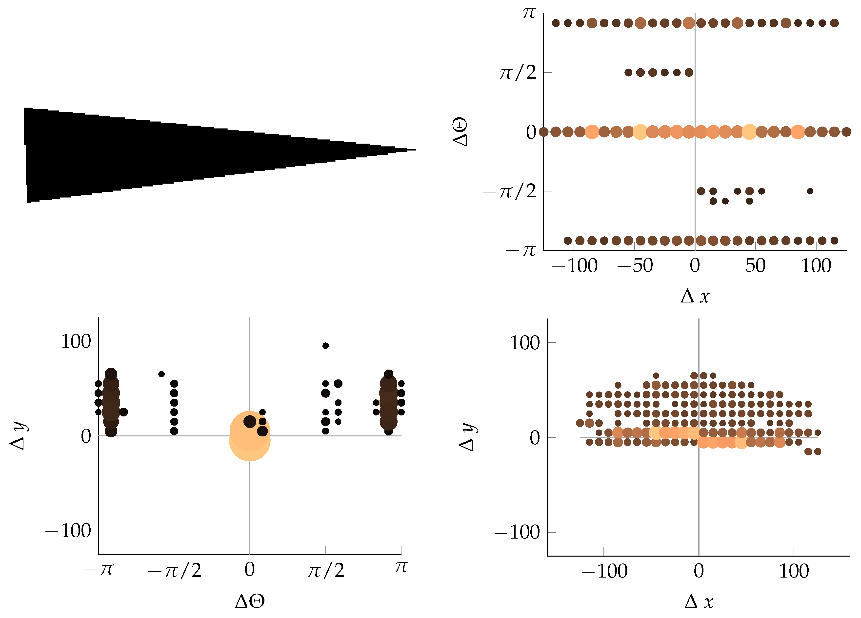
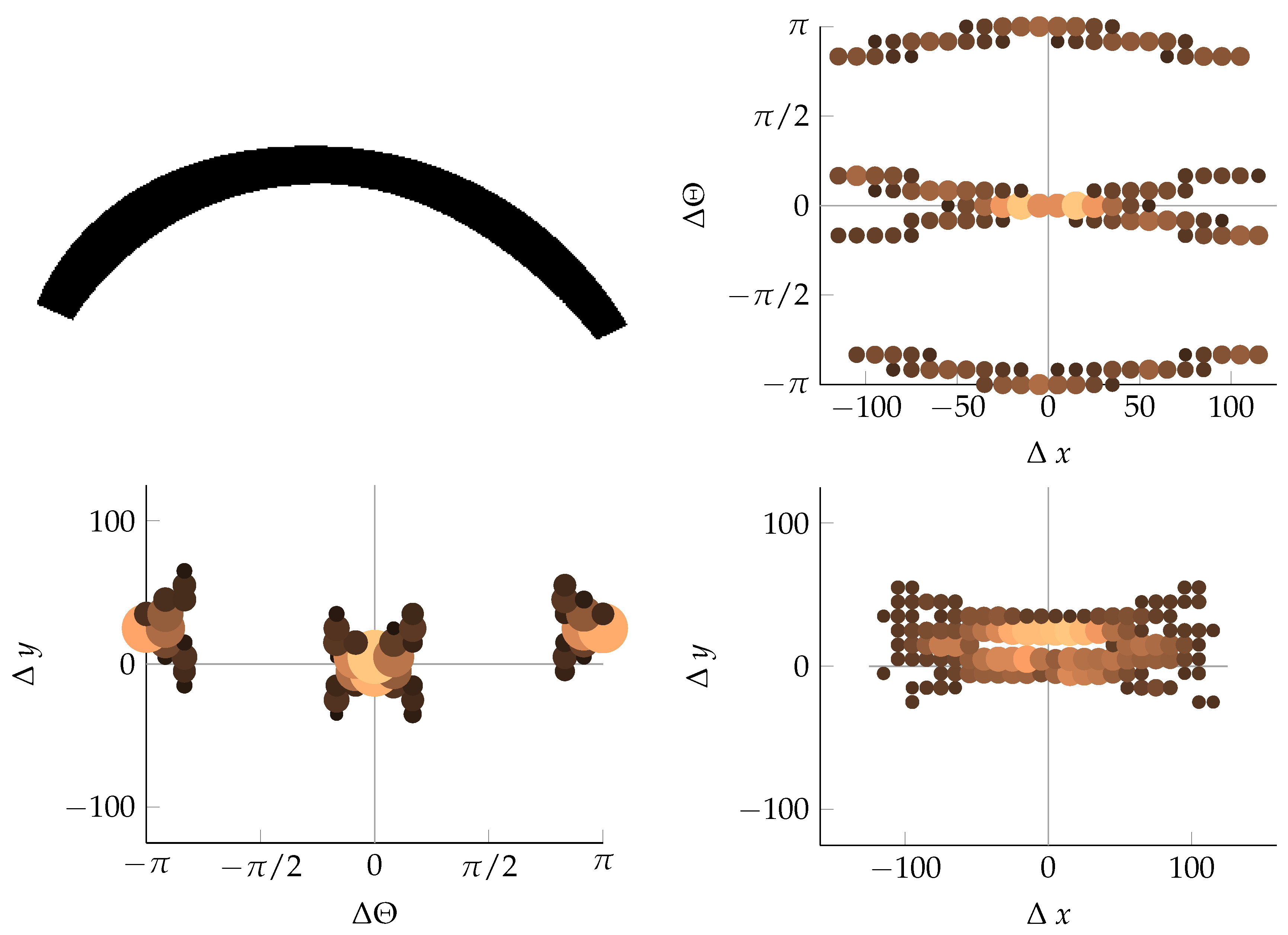
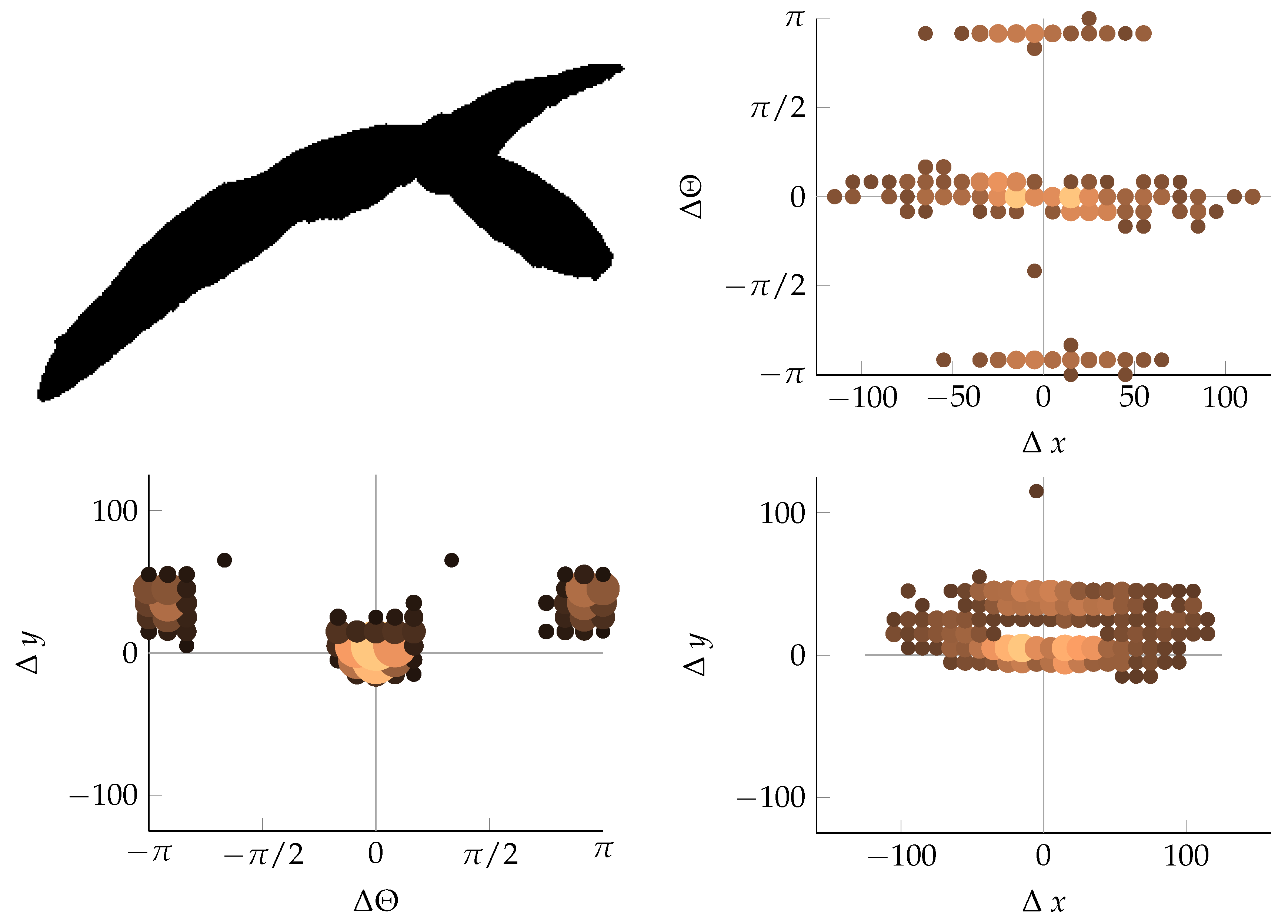
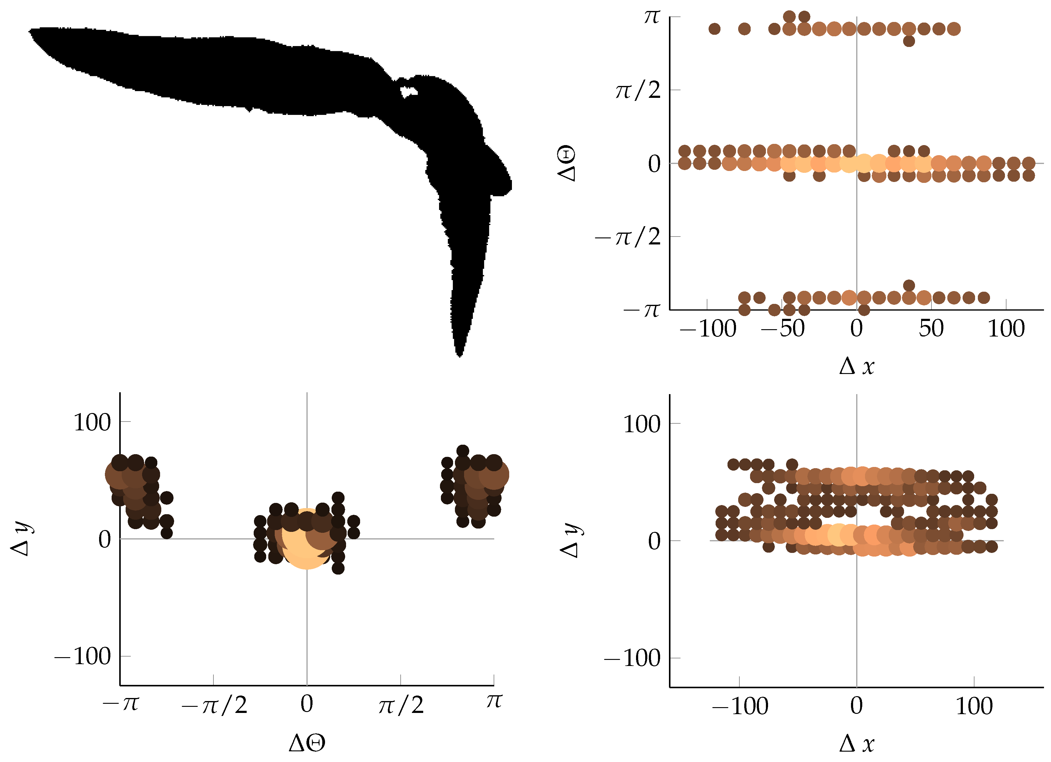
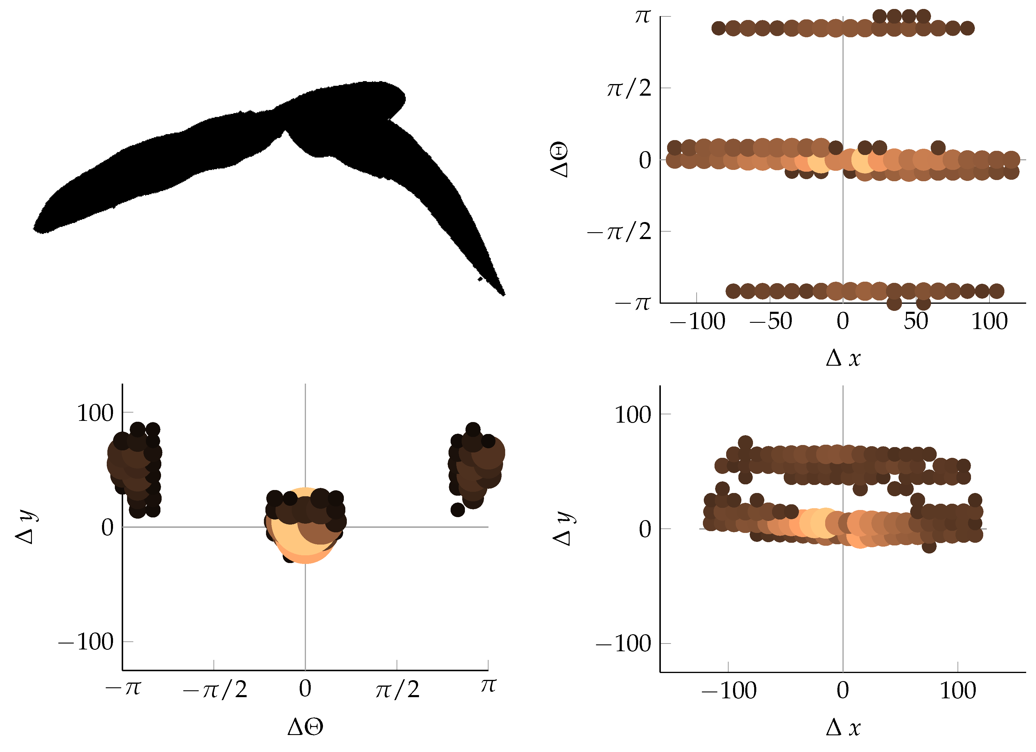
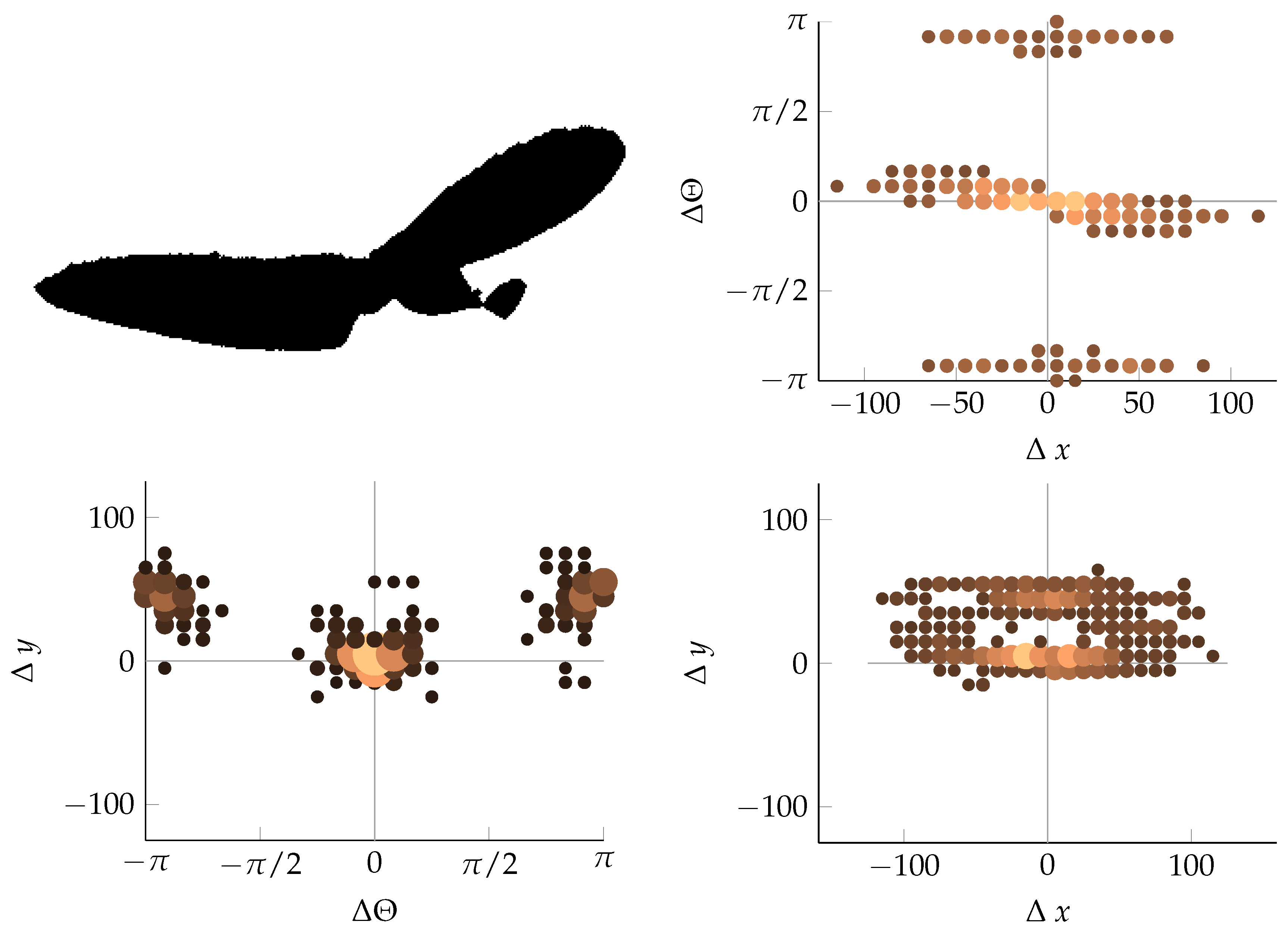
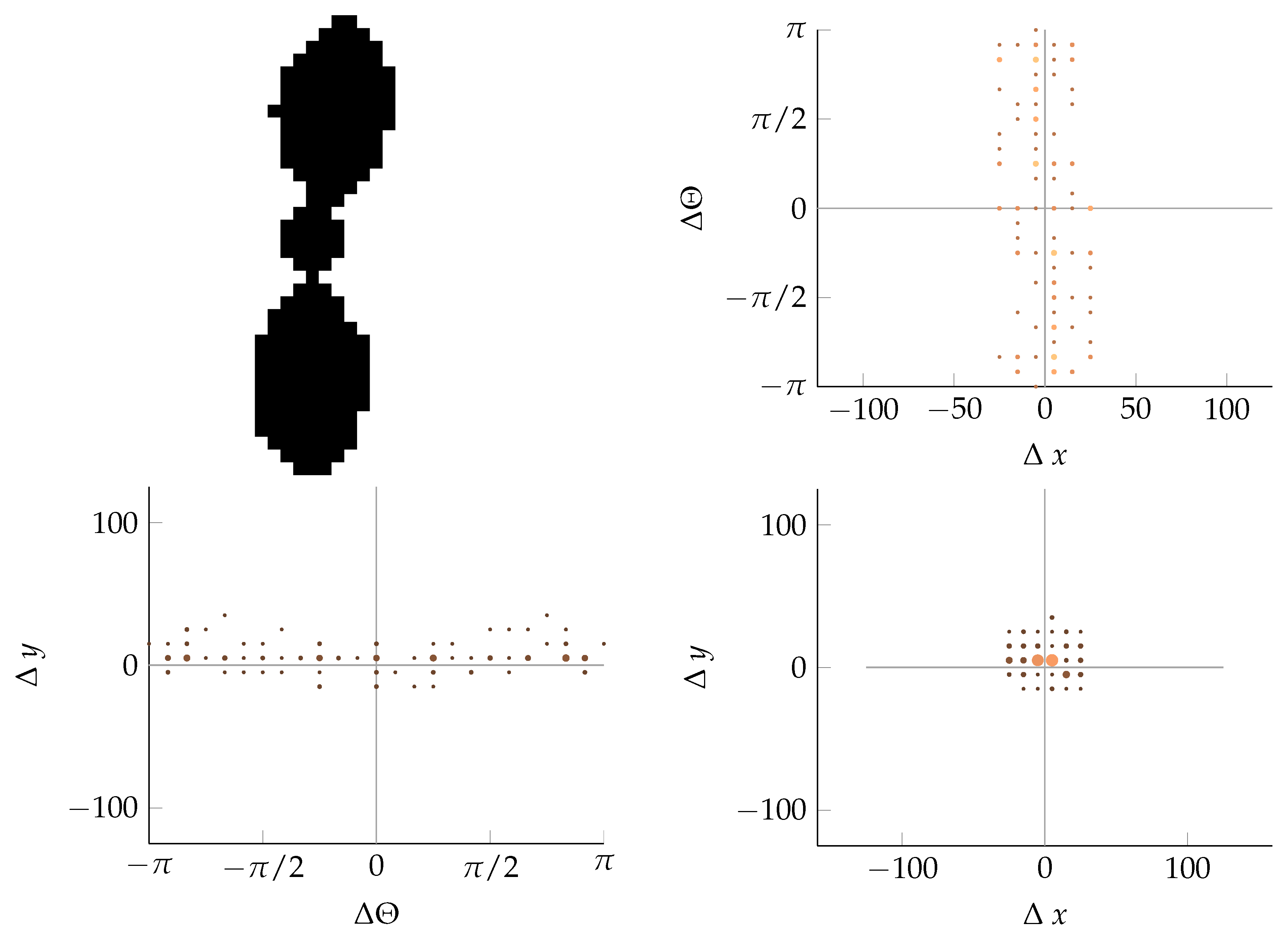
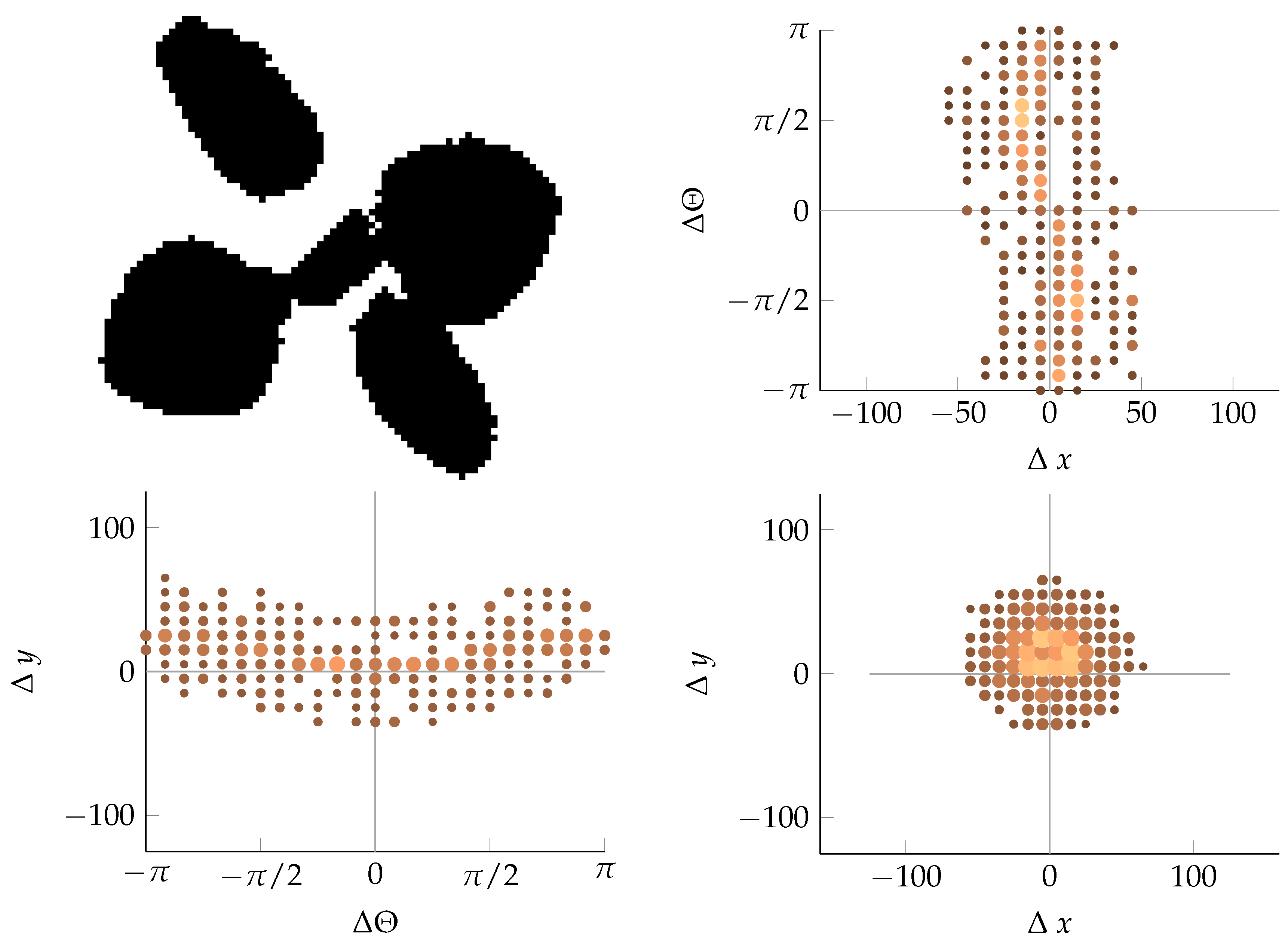
Appendix B. Example of Shapes as Seen in Relative Coordinates


References
- Kurstjens, D.A.G. Precise tillage systems for enhanced non-chemical weed management. Soil Tillage Res. 2007, 97, 293–305. [Google Scholar] [CrossRef]
- Carter. Herbicide movement in soils: Principles, pathways and processes. Weed Res. 2000, 40, 113–122. [Google Scholar]
- Thorling, L.; Brüsch, W.; Hansen, B.; Langtofte, C.; Mielby, S.; Møller, R.R. Grundvand. Status og Udvikling 1989–2011; GEUS: Copenhagen, Denmark, 2012. [Google Scholar]
- Cardina, J.; Johnson, G.A.; Sparrow, D.H. The nature and consequence of weed spatial distribution. Weed Sci. 1997, 45, 364–373. [Google Scholar]
- Thornton, P.K.; Fawcett, R.H.; Dent, J.B.; Perkins, T.J. Spatial weed distribution and economic thresholds for weed control. Crop Prot. 1990, 9, 337–342. [Google Scholar] [CrossRef]
- Lutman, P.; Miller, P. Spatially Variable Herbicide Application Technology; Opportunities for Herbicide Minimisation and Protection of Beneficial Weeds; Home-Grown Cereals Authority: Bedford, UK, 2007. [Google Scholar]
- Gerhards, R.; Christensen, S. Real-time weed detection, decision making and patch spraying in maize, sugarbeet, winter wheat and winter barley. Weed Res. 2003, 43, 385–392. [Google Scholar] [CrossRef]
- Gerhards, R. Site-specific weed control. In Precision in Crop Farming; Springer: Dordrecht, The Netherlands, 2013; pp. 273–294. [Google Scholar]
- Tian, L.; Steward, B.; Tang, L. Smart sprayer project: Sensor-based selective herbicide application system. Biol. Qual. Precis. Agric. 2000, 4203, 73–80. [Google Scholar]
- Christensen, S.; Søgaard, H.T.; Kudsk, P.; Nørremark, M.; Lund, I.; Nadimi, E.S.; Jørgensen, R. Site-specific weed control technologies. Weed Res. 2009, 49, 233–241. [Google Scholar] [CrossRef]
- Lemieux, C.; Vallee, L.; Vanasse, A. Predicting yield loss in maize fields and developing decision support for post-emergence herbicide applications. Weed Res. 2003, 43, 323–332. [Google Scholar] [CrossRef]
- Berge, T.W.; Goldberg, S.; Kaspersen, K.; Netland, J. Towards machine vision based site-specific weed management in cereals. Comput. Electron. Agric. 2012, 81, 79–86. [Google Scholar] [CrossRef]
- Miller, P.; Tillett, N.; Hague, T.; Lane, A. The development and field evaluation of a system for the spot treatment of volunteer potatoes in vegetable crops. In Proceedings of the International Advances in Pesticide Application, Wageningen, The Netherlands, 10–12 January 2012.
- Nieuwenhuizen, A.T.; Hofstee, J.W.; van Henten, E.J. Performance evaluation of an automated detection and control system for volunteer potatoes in sugar beet fields. Biosyst. Eng. 2010, 107, 46–53. [Google Scholar] [CrossRef]
- Søgaard, H.T.; Lund, I. Application accuracy of a machine vision-controlled robotic micro-dosing system. Biosyst. Eng. 2007, 96, 315–322. [Google Scholar] [CrossRef]
- Midtiby, H.S.; Mathiassen, S.K.; Andersson, K.J.; Jørgensen, R.N. Performance evaluation of a crop/weed discriminating microsprayer. Comput. Electron. Agric. 2011, 77, 35–40. [Google Scholar] [CrossRef]
- Burgos-Artizzu, X.P.; Ribeiro, A.; Guijarro, M.; Pajares, G. Real-time image processing for crop/weed discrimination in maize fields. Comput. Electron. Agric. 2011, 75, 337–346. [Google Scholar] [CrossRef] [Green Version]
- Lamm, R.D.; Slaughter, D.C.; Giles, D.K. Precision Weed Control System for Cotton. Trans. ASAE 2002, 45, 231–248. [Google Scholar]
- Slaughter, D.C. The Biological Engineer: Sensing the Difference Between Crops and Weeds. In Automation: The Future of Weed Control in Cropping Systems; Springer: Dordrecht, The Netherlands, 2014; pp. 71–95. [Google Scholar]
- Slaughter, D.C. Automation: The Future of Weed Control in Cropping Systems; Springer: Dordrecht, The Netherlands, 2014. [Google Scholar]
- Slaughter, D.C.; Giles, D.K.; Downey, D. Autonomous robotic weed control systems: A review. Comput. Electron. Agric. 2008, 61, 63–78. [Google Scholar] [CrossRef]
- Joergensen, R.N.; Krueger, N.; Midtiby, H.S.; Laursen, M.S. Spray Boom for Selectively Spraying a Herbicidal Composition onto Dicots. U.S. Patent 20140001276, 2 January 2014. [Google Scholar]
- Kropff, M.J.; Spitters, C.J. A simple model of crop loss by weed competition from early observations on relative leaf area of the weeds. Weed Res. 1991, 31, 97–105. [Google Scholar] [CrossRef]
- Jensen, K.; Laursen, M.S.; Midtiby, H.; Nyholm Jørgensen, R. Autonomous precision spraying trials using a novel cell spray implement mounted on an armadillo tool carrier. In Proceedings of the XXXV CIOSTA & CIGR V Conference, Billund, Denmark, 3–5 July 2013.
- Woebbecke, D.M.; Meyer, G.E.; Bargen, K.V.; Mortensen, D.A. Color indices for weed identification under various soil, residue, and lighting conditions. Trans. ASAE 1995, 38, 259–269. [Google Scholar] [CrossRef]
- Laursen, M.S.; Midtiby, H.; Jørgensen, R.N.; Krüger, N. Validation of Modicovi-Monocot and Dicot Coverage Ration Vision based method for real time estimation of Canopy Coverage Ration between Cereal Crops and Dicotyledon Weeds. In Proceedings of the International Conference on Precision Agriculture, Indianapolis, IN, USA, 15–18 July 2012.
- Bigun, J. Vision with Direction; Springer: Berlin/Heidelberg, Germany, 2006. [Google Scholar]
- Ali, A.; Streibig, J.C.; Christensen, S.; Andreasen, C. Estimation of weeds leaf cover using image analysis and its relationship with fresh biomass yield of maize under field conditions. In Proceedings of the 5th International Conference on Information and Communication Technologies for Sustainable Agri-Production and Environment (HAICTA 2011), Skiathos, Greece, 8–11 September 2011.
- Jensen, K.; Larsen, M.; Nielsen, S.; Larsen, L.; Olsen, K.; Jørgensen, R. Towards an open software platform for field robots in precision agriculture. Robotics 2014, 3, 207–234. [Google Scholar] [CrossRef] [Green Version]
- Laursen, M.S.; Midtiby, H.; Jørgensen, R. Improving the segmentation for weed recognition applications based on standard RGB cameras using optical filters. In Proceedings of the Agromek and NJF Joint Seminar, Herning, Denmark, 24–25 November 2014.
- Laursen, M.S.; Midtiby, H.S.; Krüger, N.; Jørgensen, R.N. Statistics-based segmentation using a continuous-scale naive Bayes approach. Comput. Electron. Agric. 2014, 109, 271–277. [Google Scholar] [CrossRef]
- Tardif-Paradis, C.; Simard, M.J.; Leroux, G.D.; Panneton, B.; Nurse, R.E.; Vanasse, A. Effect of planter and tractor wheels on row and inter-row weed populations. Crop Prot. 2015, 71, 66–71. [Google Scholar] [CrossRef]
- Timmermann, C.; Gerhards, R.; Kühbauch, W. The economic impact of site-specific weed control. Precis. Agric. 2003, 4, 249–260. [Google Scholar] [CrossRef]
- Gerhards, R.; Oebel, H. Practical experiences with a system for site-specific weed control in arable crops using real-time image analysis and GPS-controlled patch spraying. Weed Res. 2006, 46, 185–193. [Google Scholar] [CrossRef]
- Stefan, L.; Bavo, D.; Andy, L.; Nicolaas, T. Hyperspectral imager development using direct deposition of interference filters. In Proceedings of the Small Satellites Systems and Services Symposium, Majorca, Spain, 26–30 May 2014.


© 2016 by the authors; licensee MDPI, Basel, Switzerland. This article is an open access article distributed under the terms and conditions of the Creative Commons Attribution (CC-BY) license (http://creativecommons.org/licenses/by/4.0/).
Share and Cite
Laursen, M.S.; Jørgensen, R.N.; Midtiby, H.S.; Jensen, K.; Christiansen, M.P.; Giselsson, T.M.; Mortensen, A.K.; Jensen, P.K. Dicotyledon Weed Quantification Algorithm for Selective Herbicide Application in Maize Crops. Sensors 2016, 16, 1848. https://doi.org/10.3390/s16111848
Laursen MS, Jørgensen RN, Midtiby HS, Jensen K, Christiansen MP, Giselsson TM, Mortensen AK, Jensen PK. Dicotyledon Weed Quantification Algorithm for Selective Herbicide Application in Maize Crops. Sensors. 2016; 16(11):1848. https://doi.org/10.3390/s16111848
Chicago/Turabian StyleLaursen, Morten Stigaard, Rasmus Nyholm Jørgensen, Henrik Skov Midtiby, Kjeld Jensen, Martin Peter Christiansen, Thomas Mosgaard Giselsson, Anders Krogh Mortensen, and Peter Kryger Jensen. 2016. "Dicotyledon Weed Quantification Algorithm for Selective Herbicide Application in Maize Crops" Sensors 16, no. 11: 1848. https://doi.org/10.3390/s16111848