
Achieving Passive Localization with Traffic Light Schedules in Urban Road Sensor Networks

Abstract
:1. Introduction
- A novel localization scheme is presented based on the position of public facilities. To our best of knowledge, the TLS algorithm is the first localization scheme that employs the public facilities information.
- The localization is accomplished using only the binary detection of vehicles in an urban road network. Unlike previous approaches, TLS is designed especially for sparse sensor networks where long-distance ranging is difficult. In addition, some practical issues are considered, such as a similar traffic light schedule and some damaged nodes.
- A novel method for calculating the similarity of two matrices is designed. This method can judge the similarity of two matrices even when the row order of a matrix is uncertain.
- The performance of the proposed design is evaluated by extensive simulation studies. The results show that our localization scheme can work well.
2. Related Work
3. Problem Formulation
3.1. Definitions
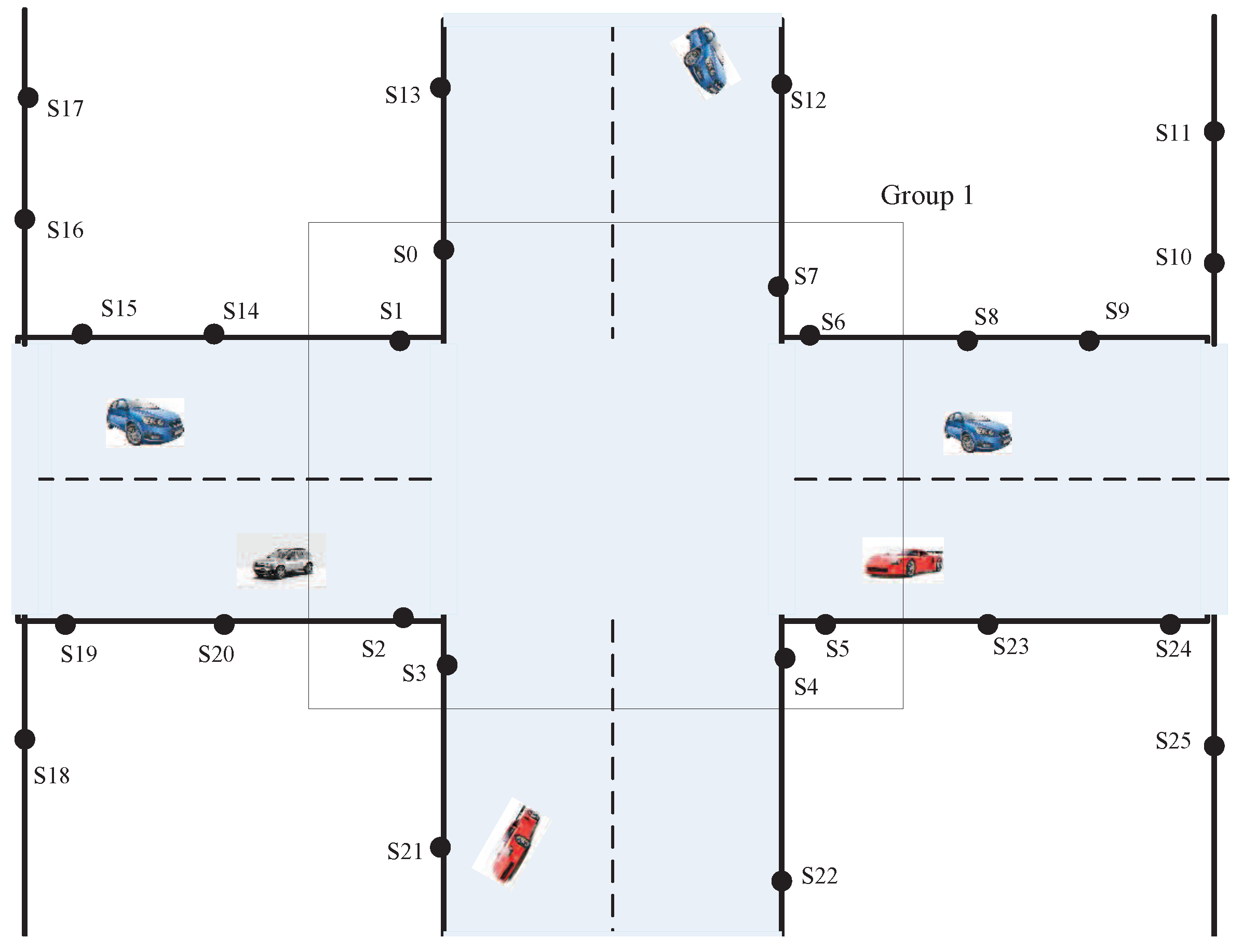
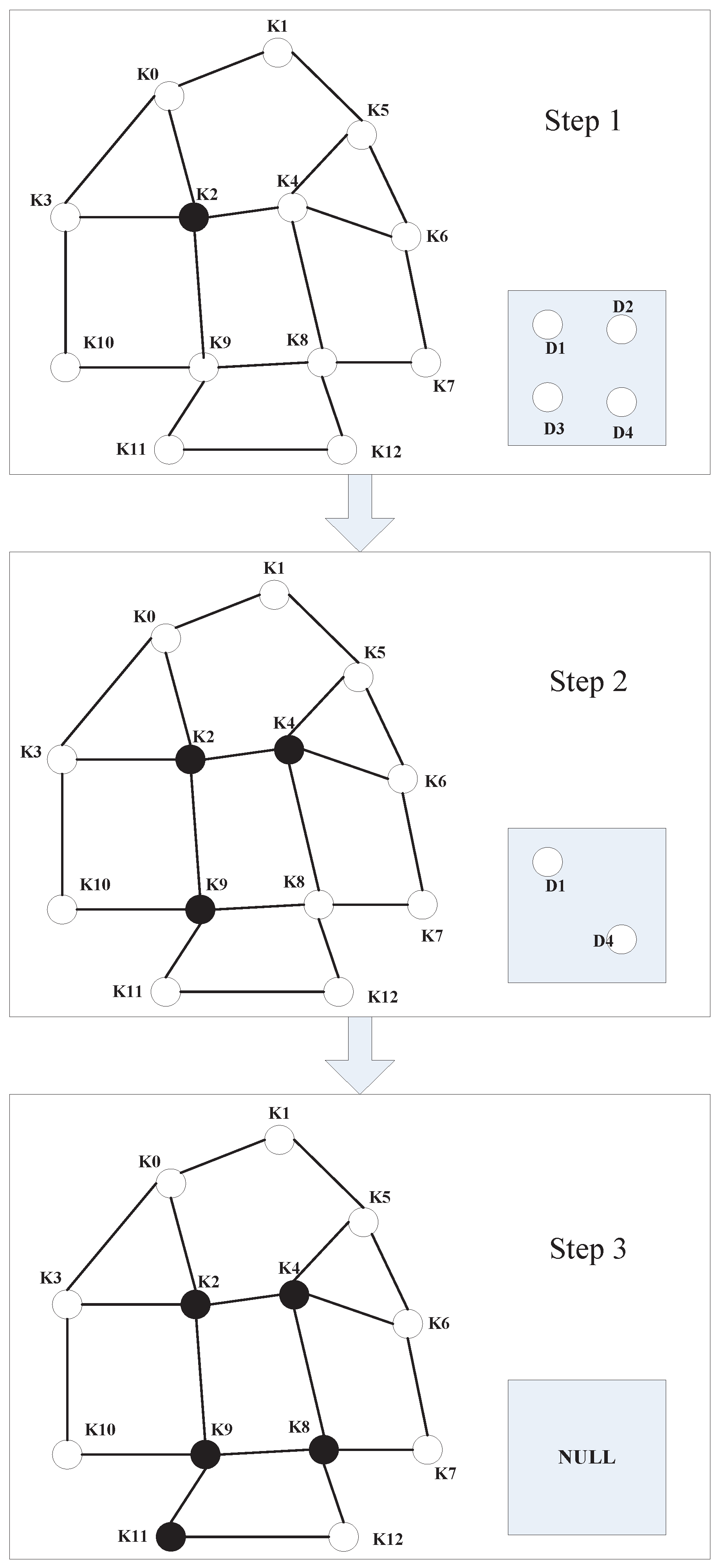
- Intersection node group: We choose eight sensors near the intersection as a group. This sensor group is called the intersection node group. In Figure 1, sensors and compose an intersection node group.
- Key nodes: Sensors are placed at intersections. These sensors belong to an intersection node group. In Figure 1, sensors and are key nodes.
- Common nodes: Sensors are placed at non-intersections. These sensors do not belong to any intersection node group. In Figure 1, sensors and are common nodes.
- Detection matrix collection: Analysis of data collected by each intersection node group, which constructs a detection matrix. All of the detection matrices compose the detection matrix collection.
- Known matrix collection: Using the intersection traffic light information that is obtained from the transport sector, we can construct a known matrix for each intersection. All of the known matrices compose the known matrix collection.
- TLS server: A computer that performs the localization algorithm with binary vehicle detection time stamps collected from the sensor network.
3.2. Assumptions
- Sensors have simple sensing devices without any costly ranging or GPS devices. Each detection is a tuple consisting of a sensor ID , intersection node group ID and time stamp . For the common nodes not belonging to any intersection node group, the tuple is sent to the TLS server.
- The traffic light information of the target area is shown on the TLS server. The information consists of traffic time seconds and of a traffic light’s location.
- Sensors deployed in the road on both sides so that each intersection is guaranteed to have one intersection node group.
- Each intersection node group of eight nodes is close to the intersection so that the key nodes and intersection location are basically identical.
- An existing ad hoc network consisting of sensors or a Delay-Tolerant Network (DTN) for wireless sensors aims to deliver vehicle-detection time stamps to the TLS server. For such a DTN, utilizing the Vehicular Ad Hoc Network (VANET) forwarding schemes, such as Vehicle-Assisted Data Delivery(VADD) [13] and Trajectory-Based Data(TBD) [38], to deliver the time stamps to the TLS server, VANETs are constructed by the vehicles, which are data mules [39].
- Sensors are time-synchronized at the millisecond level. We can use the time synchronization protocol in [40] to ensure the time synchronization accuracy in sparse urban road sensor networks; since the time synchronization protocol in [40] is the start-of-the-art time synchronization protocol for spare wireless sensor networks and can ensure the time-synchronized at the millisecond level.
4. TLS System Design
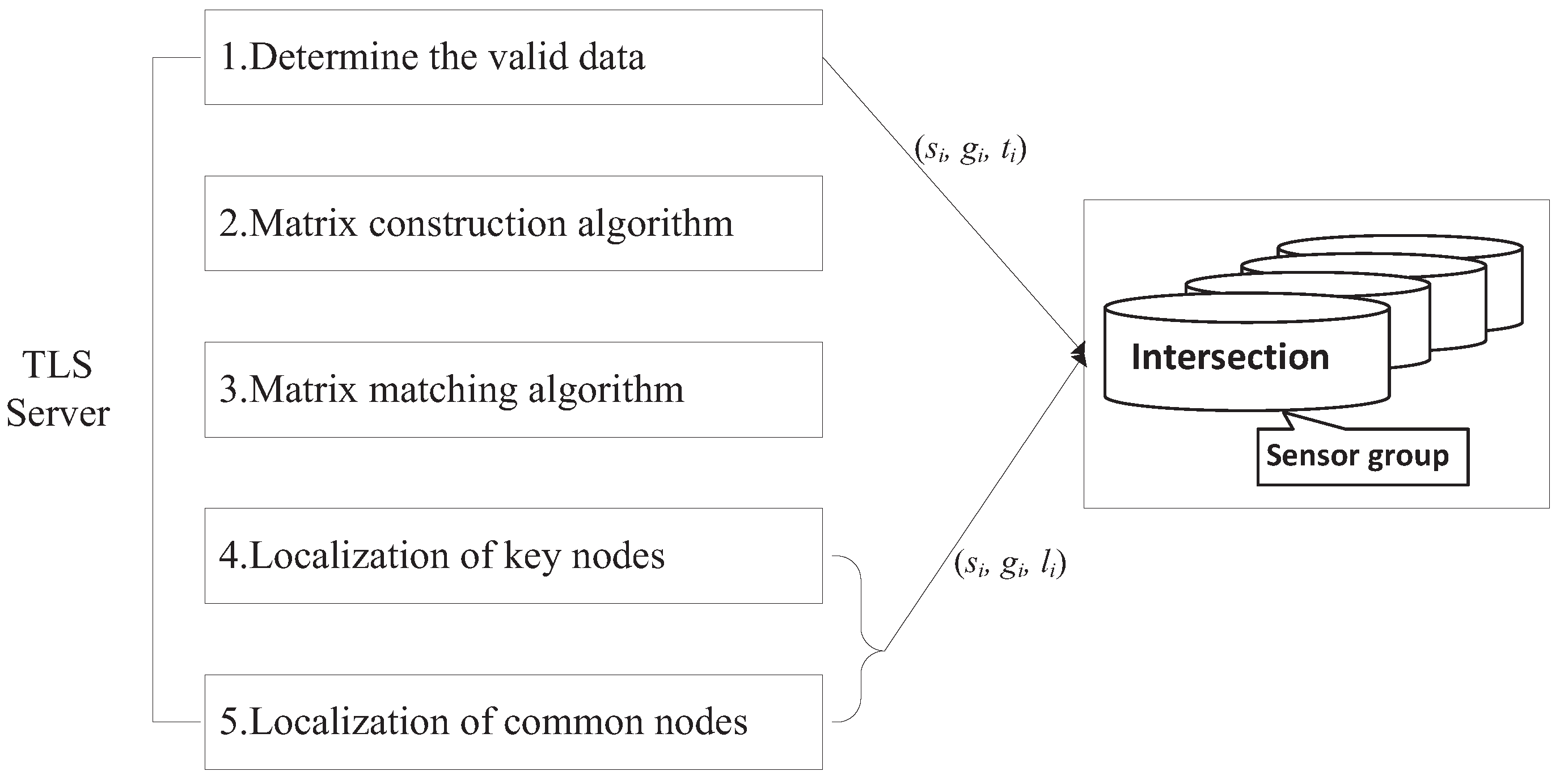
4.1. System Architecture
- Step 1. After road traffic measurement, sensors send a tuple to the TLS server, i.e., , where is the sensor ID, is the intersection node group ID and is a time stamp.
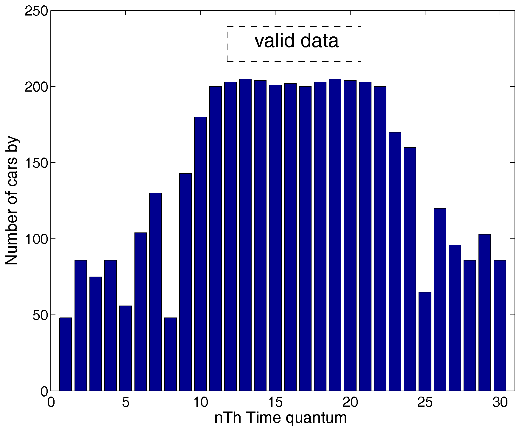
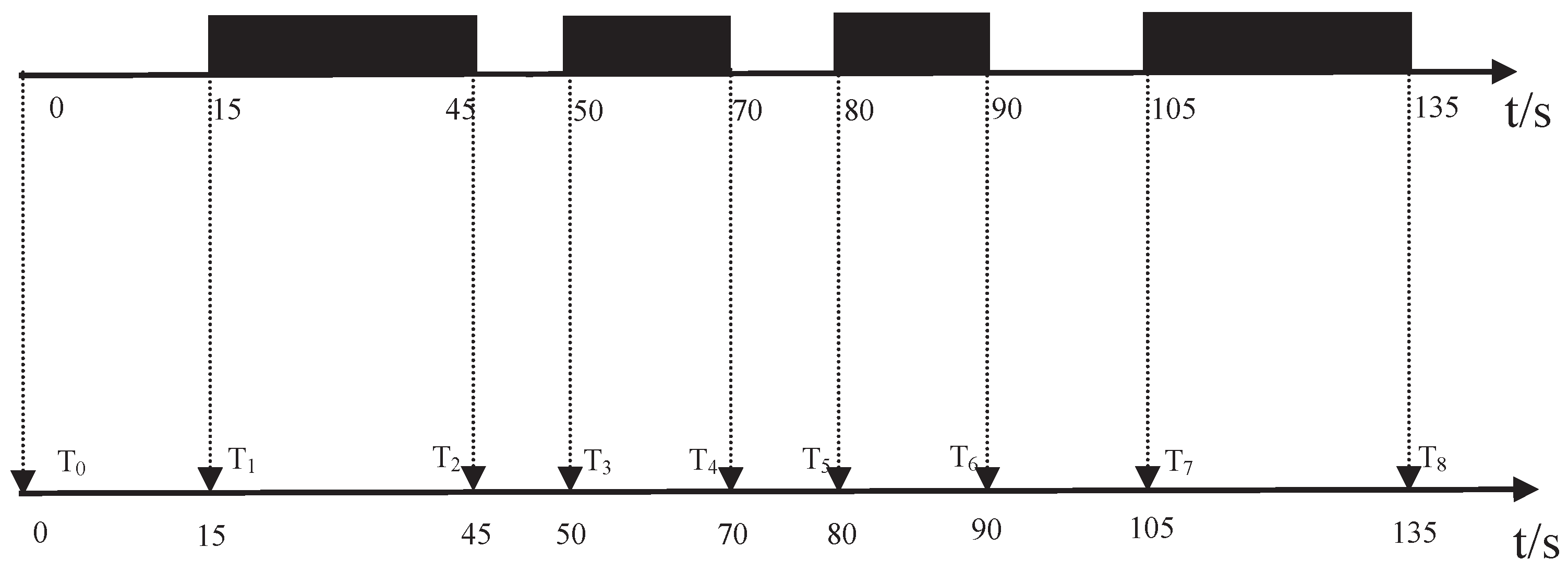
- Step 2. Determining the valid data: The data collected in the heavy traffic time is regarded as valid data, because the time period with cars on the road and the time period without cars is a regular cycle. In the following, a method is designed to screen out the valid data.
- Step 3. By using valid data collected from nodes, the information from each intersection node group can be used to construct a detection matrix. These matrices constitute the detection matrix collection.
- Step 4. We use our algorithm to determine the similar matrix in detection matrix collection and known matrix collection.
- Step 5. Because we already know the geographical location of traffic lights, we can locate the position of the key nodes according to the matrix matching results (obtained from Step 4), and then, we can use the APL algorithm to locate the position of the common nodes.
- Step 6. The TLS server sends each sensor its location with a message .
4.2. Step 2: Determine the Valid Data
4.2.1. Determining the Valid Data Operation
4.2.2. Analysis of Determining Valid Data Errors
4.3. Step 3: Matrix Construction Algorithm
4.3.1. Detection Matrix Construction Algorithm
4.3.2. Known Matrix Construction Algorithm
4.4. Step 4: Matrix Matching Algorithms
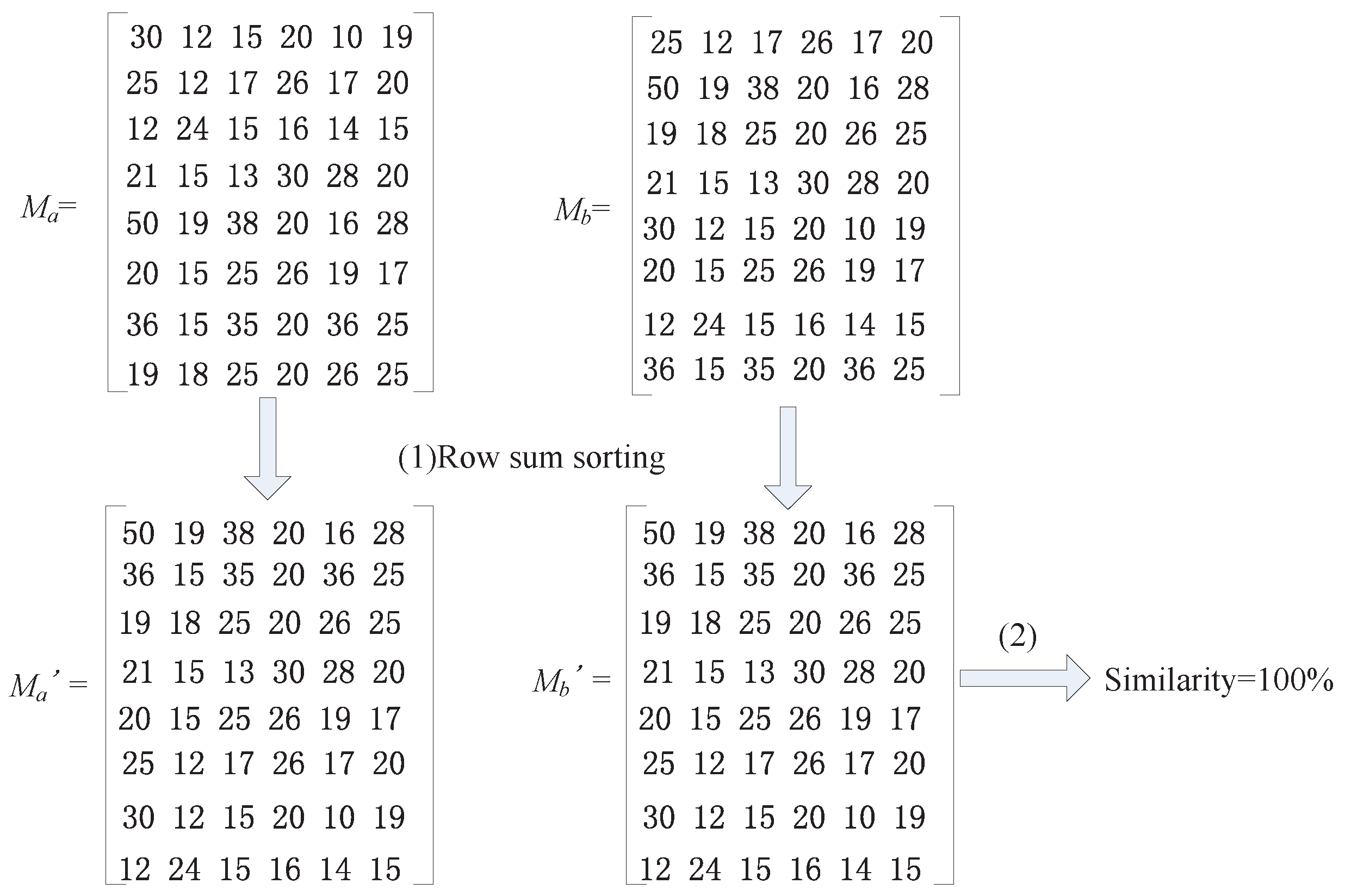
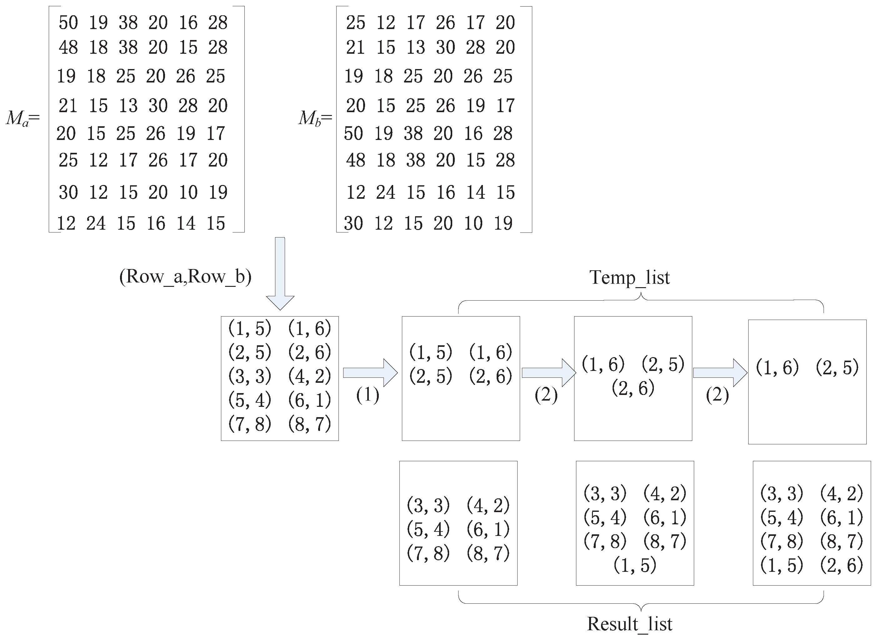
4.4.1. Calculate the Similarity of the Matrix
4.4.2. Row Uncertain Matrix Matching Algorithm
(a) Row Sum Sorting Method (RSS)
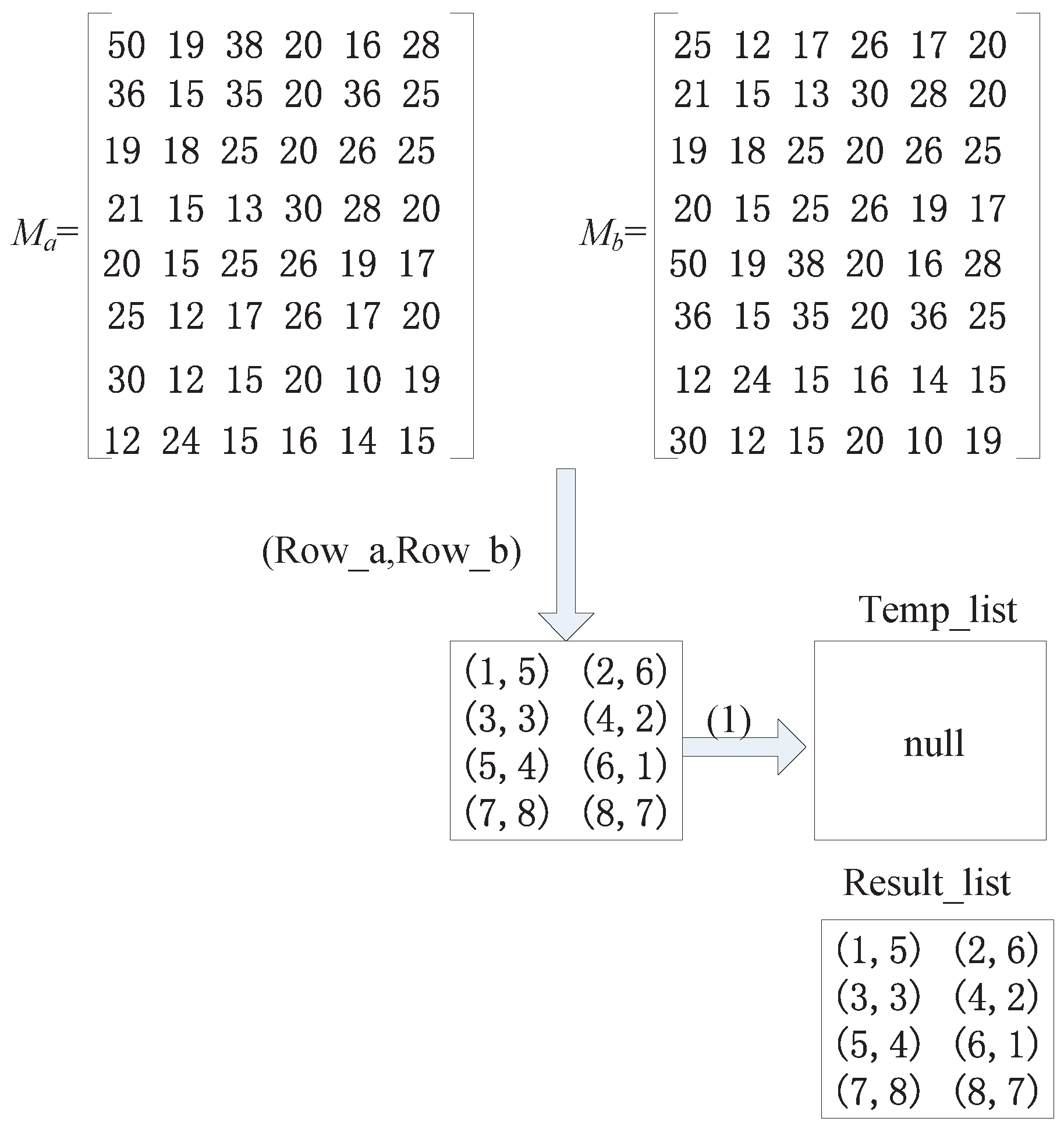
(b) Calculate the Similarity by the Unit of Lines (SUL) Method
- Step 1. Find the line number groups in which is not repeated in the set and move these line number groups to another set for storage.
- Step 2. After performing the moving operation in the first step, if the set is not empty, we perform the second moving operation and successively determine the line number groups remaining in the set . If the and in this line number group are different from those in the set , we move this type of line number group out to , as well.
- Step 3. We determine the number of line number groups in the set . If the number equals the number of lines in the matrix, it is believed that the two matrices are similar.
4.5. Step 5: Node Location Identification
4.5.1. Localization of Key Nodes
4.5.2. Localization of Common Nodes
5. Practical Discussion
5.1. Dealing with the Same Traffic Light Schedule
- Method 1. There are not two identical matrices in the detection matrix collection, but a matrix in the detection matrix collection has more than one matching result with the matrix of the known matrix collection. Because our detection range is within a region, we can locate these special points according to the surrounding intersection node group. When constructing the known matrix collection, we assign to each matrix of a set its surrounding information. Then, we put the matrix around the matrix of the special group in the detection matrix collection to match each other. If the surrounding information in the detection matrix collection has a successful match, we can obtain the corresponding matching result of the special matrix according to the matrix information around the node.
- Method 2. When the nearby traffic lights have a similar setting or the detection matrix collection has identical matrices, the above method does not work well. Therefore, we also can use the map matching method of the APL algorithm to deal with the same traffic light schedule problem.
5.2. The Known Matrix Collection Is Very Large
- Step 1. We determine the similarity matrix of the first detection matrix () in the known matrix collection. The similarity matrix is considered as the initial matrix.
- Step 2. Once the surrounding matrix of the initial matrix is known, we determine the similarity matrix of the surrounding matrix in detection collection. If we determine the similar matrix of a given surrounding matrix, we consider this surrounding matrix as the initial matrix. Then, we perform Step 2 again. It is important to note, if all of the surrounding matrices of the initial matrix do not match, we will need to choose a new initial matrix. We repeat until all of the matrices of the detection matrix collection are matched successfully.
5.3. Some Key Nodes Damaged
5.4. Exciting Some Adaptive Traffic Light Controls
6. Performance Evaluation
6.1. Investigation on System Parameters
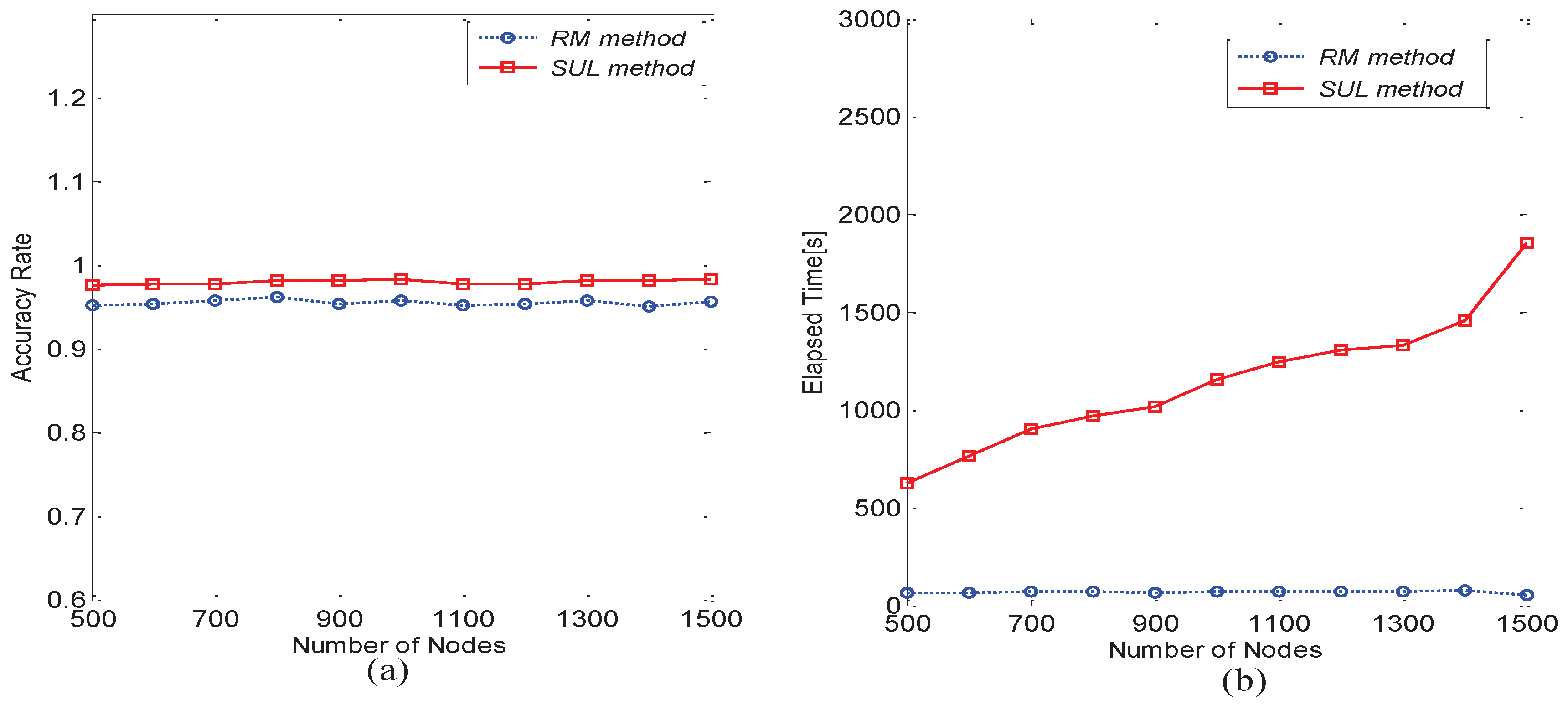
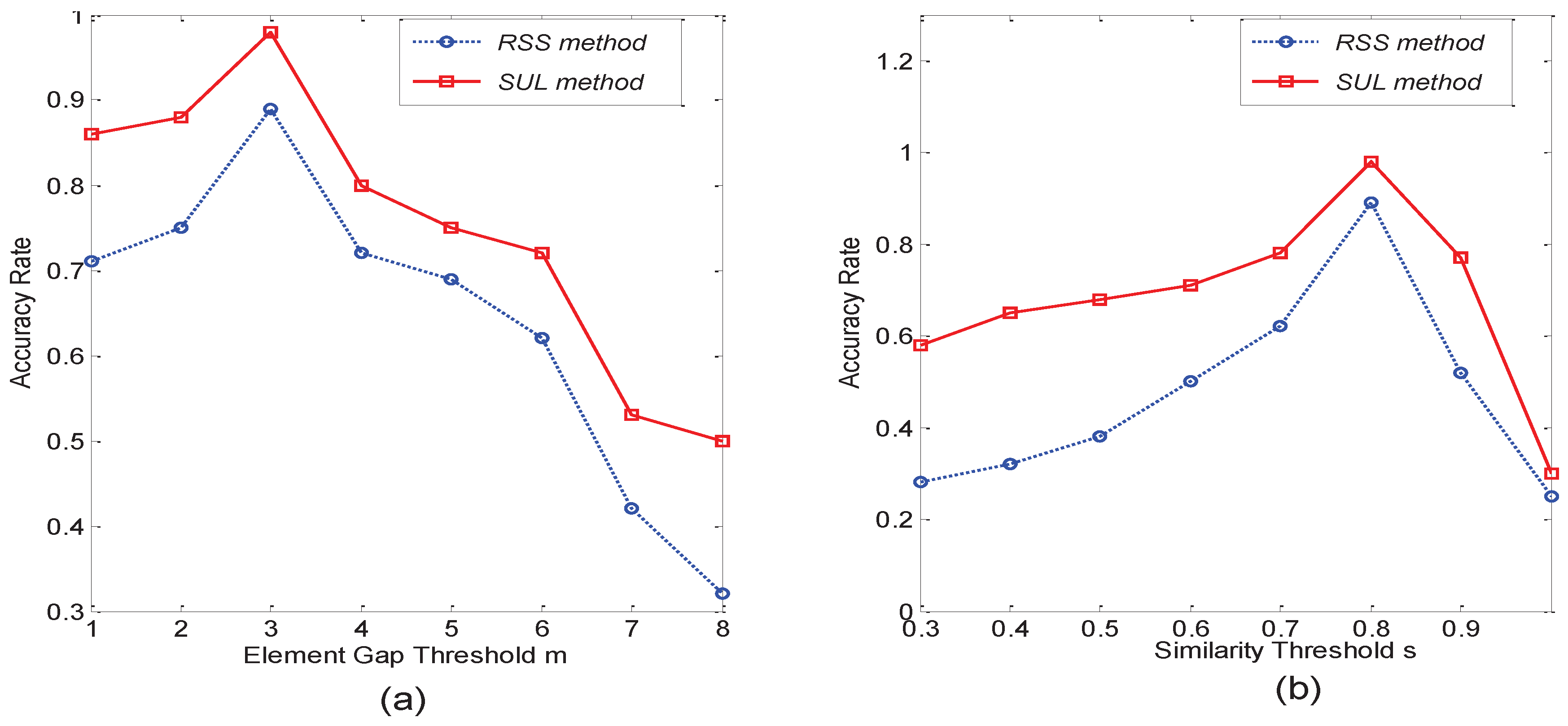
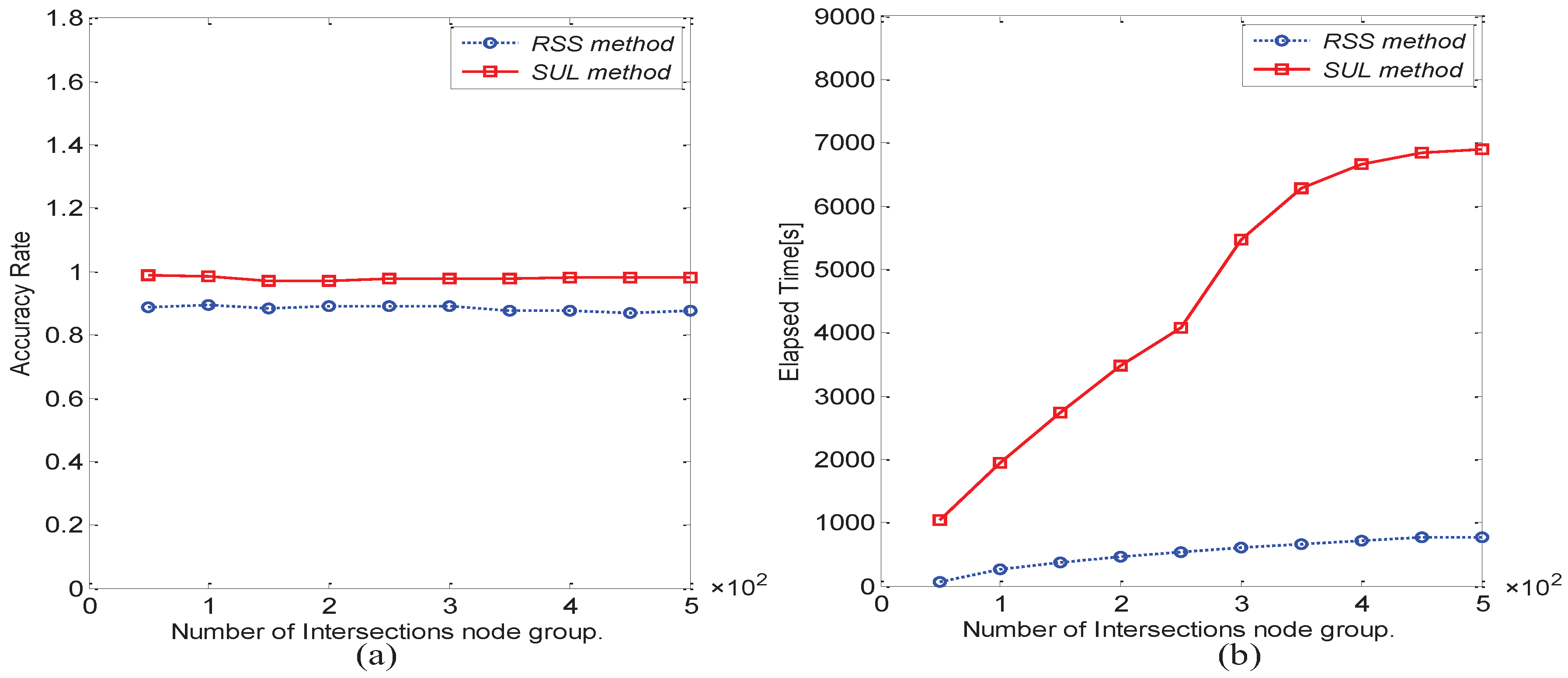
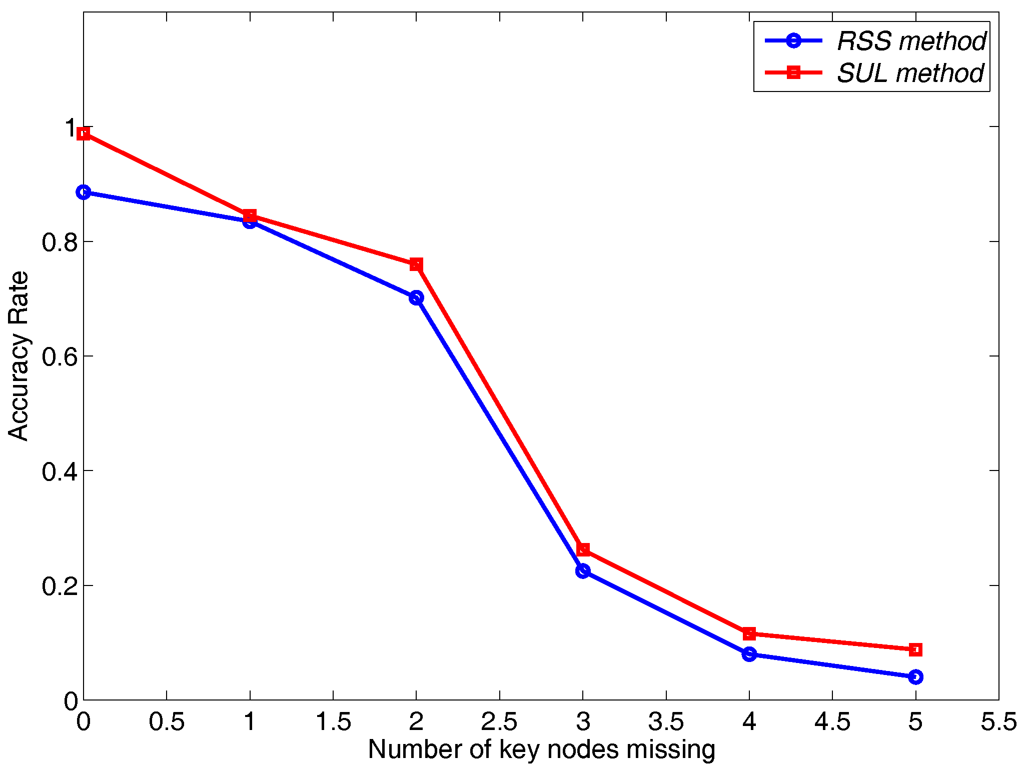
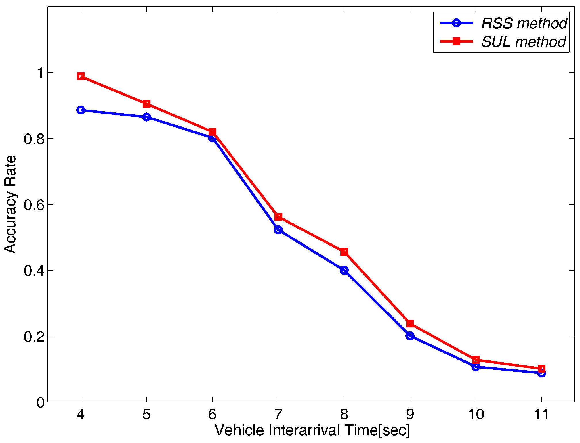
6.2. Performance Comparison between Matrix Matching Methods
- Row Sum Sorting method (RSS)
- Calculate the Similarity by the Unit of Lines method (SUL)
- Recursion Matching method (RM)
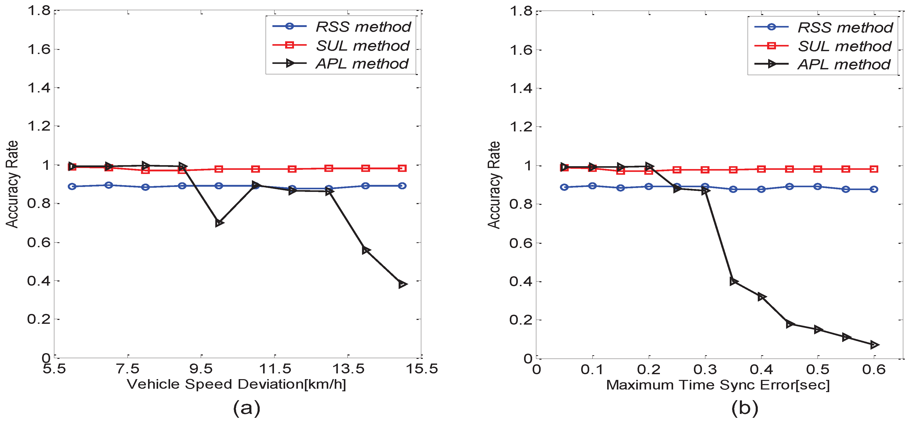
6.3. Performance Comparison between the TLS Algorithm and the APL Algorithm
6.4. Impact of Practical Factors
7. Conclusions
Acknowledgments
Author Contributions
Conflicts of Interest
References
- Bahl, P.; Padmanabhan, V.N. RADAR: An In-Building RF-Based User Location and Tracking System. In Proceedings of Nineteenth Annual Joint Conference of the IEEE Computer and Communications Societies (INFOCOM 2000), Tel Aviv, Israel, 26–30 March 2000; pp. 775–784.
- Wellenhoff, B.H.; Lichtenegger, H.; Collins, J. Global Positions System: Theory and Practice; Springer: Wien, Austria, 1997. [Google Scholar]
- Priyantha, N.B.; Chakraborty, A.; Balakrishnan, H. The Cricket Location-Support System. In Proceedings of the 6th Annual International Conference on Mobile Computing and Networking, Boston, MA, USA, 6–11 August 2000.
- Niculescu, D.; Nath, B. Ad Hoc Positioning System (APS) Using AOA. In Proceedings of the Twenty-Second Annual Joint Conference of the IEEE Computer and Communications (INFOCOM 2003), San Francisco, CA, USA, 30 March–3 Apirl 2003.
- Bulusu, N.; Heidemann, J.; Estrin, D. GPS-Less Low Cost Outdoor Localization for Very Small Devices. IEEE Pers. Commun. 2000, 7, 28–34. [Google Scholar] [CrossRef]
- Moore, D.; Leonard, J.; Rus, D.; Teller, S. Robust Distributed Network Localization with Noise Range Measurements. In Proceedings of the 2nd International Conference on Embedded Networked Sensor Systems, Baltimore, MA, USA, 3–5 November 2004.
- Lazos, L.; Poovendran, R. SeRLoc: Secure Range-Independent Localization for Wireless Sensor Networks. In Proceedings of the 3rd ACM Workshop on Wireless Security, Philadelphia, PA, USA, 1 October 2004.
- He, T.; Huang, C.; Blum, B.M.; Stankovic, J.A.; Abdelzaher, T. Range-Free Localization Schemes for Large-Scale Sensor Networks. In Proceedings of the 9th Annual International Conference on Mobile Computing and Networking, San Diego, CA, USA, 14–19 September 2003.
- Shang, Y.; Ruml, W.; Zhang, Y.; Fromherz, M.P.J. Localization from Mere Connectivity. In Proceedings of the 4th ACM International Symposium on Mobile Ad Hoc Networking and Computing, Annapolis, MD, USA, 1–3 June 2003.
- Gao, K.; Zhang, Y.; Su, R.; Lentzakis, A. Discrete harmony search algorithm for solving urban traffic light scheduling problem. In Proceedings of the American Control Conference, Boston, MA, USA, 6–8 July 2016.
- Gao, K.; Zhang, Y.; Sadollah, A.; Su, R. Optimizing urban traffic light scheduling problem using harmony Search with ensemble of local search. Appl. Soft Comput. 2016, 48, 359–372. [Google Scholar] [CrossRef]
- Collotta, M.; Bello, L.L.; Pau, G. A novel approach for dynamic traffic lights management based on Wireless Sensor Networks and multiple fuzzy logic controllers. Expert Syst. Appl. 2015, 42, 5403–5415. [Google Scholar] [CrossRef]
- Zhao, J.; Cao, G. VADD: Vehicle-assisted data delivery in vehicular ad hoc networks. IEEE Trans. Veh. Technol. 2008, 57, 1910–1912. [Google Scholar] [CrossRef]
- GB Traffic Volumes. Available online: www.mapmechanics.com (accessed on 30 June 2016).
- Wang, Y.; Zheng, Y.; Xue, Y. Travel Time Estimation of a Path using Sparse Trajectories. In Proceedings of the 20th SIGKDD Conference on Knowledge Discovery and Data Mining, New York, NY, USA, 24–27 August 2014; pp. 25–34.
- Yuan, J.; Zheng, Y.; Xie, X.; Sun, G. Driving with Knowledge from the Physical World. In Proceedings of the 17th SIGKDD Conference on Knowledge Discovery and Data Mining, San Diego, CA, USA, 21–24 August 2011; pp. 316–324.
- Li, Y.; Zheng, Y.; Zhang, H.; Chen, L. Traffic Prediction in a Bike Sharing System. In Proceedings of the 23rd ACM International Conference on Advances in Geographical Information Systems, Seattle, WA, USA, 3–6 November 2015.
- Liu, W.; Zheng, Y.; Chawla, S.; Yuan, J.; Xing, X. Discovering Spatio-Temporal Causal Interactions in Traffic Data Streams. In Proceedings of the 17th SIGKDD conference on Knowledge Discovery and Data Mining, San Diego, CA, USA, 21–24 August 2011; pp. 1010–1018.
- Shang, J.; Zheng, Y.; Tong, W.; Chang, E.; Yu, Y. Inferring Gas Consumption and Pollution Emission of Vehicles throughout a City. In Proceedings of the 20th SIGKDD Conference on Knowledge Discovery and Data Mining, New York, NY, USA, 24–27 August 2014; pp. 1011–1025.
- Zheng, Y.; Yi, X.; Li, M.; Li, R.; Shan, Z.; Chang, E.; Li, T. Forecasting Fine-Grained Air Quality Based on Big Data. In Proceedings of the 21th SIGKDD Conference on Knowledge Discovery and Data Mining, Sydney, Australia, 10–13 August 2015; pp. 2267–2276.
- Jeong, J.; Guo, S.; He, T.; Du, D.H. Autonomous passive localization algorithm for road sensor networks. IEEE Trans. Comput. 2011, 11, 1622–1637. [Google Scholar] [CrossRef]
- Youssef, M.; Mah, M.; Agrawala, A. Challenges: Device-Free Passive Localization for Wireless Environments. In Proceedings of the 13th Annual ACM International Conference on Mobile Computing and Networking, Montreal, QC, Canada, 9–14 September 2007.
- Zhou, G.; He, T.; Krishnamurthy, S.; Stankovic, J.A. Impact of Radio Irregularity on Wireless Sensor Networks. In Proceedings of the 2nd International Conference on Mobile Systems, Applications, and Services, Boston, MA, USA, 6–9 June 2004.
- Niculescu, D.; Nath, B. DV Based Positioning in Ad Hoc Networks. Telecommun. Syst. 2003, 22, 267–280. [Google Scholar] [CrossRef]
- Chen, P.; Ma, H.; Gao, S.; Huang, Y. Modified Extended Kalman Filtering for Tracking with Insufficient and Intermittent Observations. Math. Prob. Eng. 2015, 2015, 981727. [Google Scholar] [CrossRef]
- Lederer, S.; Wang, Y.; Gao, J. Connectivity-Based Localization of Large Scale Sensor Networks with Complex Shape. ACM Trans. Sens. Netw. 2009, 5, 31. [Google Scholar] [CrossRef]
- Bulusu, N.; Heidemann, J.; Estrin, D.; Tran, T. Self-Configuring Localization Systems: Design and Experimental Evaluation. ACM Trans. Embedded Comput. Syst. 2004, 3, 24–60. [Google Scholar] [CrossRef]
- Nagpal, R.; Shrobe, H.; Bachrach, J. Organizing a Global Coordinate System from Local Information on an Ad Hoc Sensor Network. In Information Processing in Sensor Networks; Springer: Berlin/Heidelberg, Germeny, 2016; pp. 333–348. [Google Scholar]
- Rabaey, C.S.J.; Langendoen, K. Robust Positioning Algorithms for Distributed Ad-Hoc Wireless Sensor Networks. In Proceedings of the 2002 USENIX Annual Technical Conference, Monterey, CA, USA, 10–15 June 2002.
- Chen, P.; Ma, H.; Gao, S.; Huang, Y. SSL: Signal Similarity-Based Localization for Ocean Sensor Networks. Sensors 2015, 15, 29702–29720. [Google Scholar] [CrossRef] [PubMed]
- Zhong, Z.; He, T. MSP: Multi-Sequence Positioning of Wireless Sensor Nodes. In Proceedings of the 5th International Conference on Embedded Networked Sensor Systems, Sydney, Australia, 6–9 November 2007.
- Zhong, Z.; Wang, D.; He, T. Sensor Node Localization Using Uncontrolled Events. In Proceedings of the 28th International Conference on Distributed Computing Systems, Beijing, China, 17–20 June 2008.
- Stoleru, R.; He, T.; Stankovic, J.A.; Luebke, D. A High-Accuracy, Low-Cost Localization System for Wireless Sensor Networks. In Proceedings of the 3rd International Conference on Embedded Networked Sensor Systems, San Diego, CA, USA, 2–4 November 2005.
- Stoleru, R.; Vicaire, P.; He, T.; Stankovic, J.A. StarDust: AFlexible Architecture for Passive Localization in Wireless Sensor Networks. In Proceedings of the 4th International Conference on Embedded Networked Sensor Systems, Boulder, CO, USA, 31 October–3 November 2006.
- Römer, K. The Lighthouse Location System for Smart Dust. In Proceedings of the 1st International Conference on Mobile Systems, Applications and Services, San Francisco, CA, USA, 5–8 May 2003.
- Seifnaraghi, N.; Ebrahimi, S.G.; Ince, E.A. Novel traffic lights signaling technique based on lane occupancy rates. In Proceedings of 24th International Symposium on Computer and Information Sciences, Guzelyurt, Cyprus, 14–16 September 2009.
- Bai, L.F.; Xu, J.X. Research on Urban Traffic Signal Control Method at Single intersection. Adv. Mater. Res. 2012, 361, 1799–1802. [Google Scholar] [CrossRef]
- Jeong, J.; Guo, S.; Gu, Y.; He, T.; Du, D. TBD: Trajectory-Based Data Forwarding for Light-Traffic Vehicular Networks. In Proceedings of the 29th IEEE International Conference on Distributed Computing Systems, Montreal, QC, Canada, 22–26 June 2009; pp. 231–238.
- Jiang, C.J.; Chen, C.; Chang, J.W.; Jan, R.H.; Chiang, T.C. Construct Small Worlds in Wireless Networks Using Data Mules. In Proceedings of the IEEE International Conference on Sensor Networks, Ubiquitous and Trustworthy Computing, Taichung, Taiwan, 11–13 June 2008; pp. 28–35.
- Römer, K. Time Synchronization in Ad Hoc Networks. In Proceedings of the 2nd ACM International Symposium on Mobile Ad Hoc Networking and Computing, Long Beach, CA, USA, 4–5 October 2001.
- Wisitpongphan, N.; Bai, F.; Mudalige, P.; Tonguz, O.K. On the Routing Problem in Disconnected Vehicular Ad Hoc Networks. In Proceedings of the 26th IEEE International Conference on Computer Communications, Anchorage, AK, USA, 6–12 May 2007.
- DeGroot, M.; Schervish, M. Probability and Statistics, 4th ed.; Addison-Wesley: Boston, MA, USA, 2011; pp. 275–345. [Google Scholar]


| Parameter | Description |
|---|---|
| number of vehicle arrivals within an hour λ | represents 600 vehicles arrival within an hour. |
| Time segment t | represents a time segment of 10 min. |
| number of vehicle arrivals within time segment n | represents 200 vehicles arriving within 10 min. |
| determining valid data error probability | It represents the probability of in the sparse time segment. |
© 2016 by the authors; licensee MDPI, Basel, Switzerland. This article is an open access article distributed under the terms and conditions of the Creative Commons Attribution (CC-BY) license (http://creativecommons.org/licenses/by/4.0/).
Share and Cite
Niu, Q.; Yang, X.; Gao, S.; Chen, P.; Chan, S. Achieving Passive Localization with Traffic Light Schedules in Urban Road Sensor Networks. Sensors 2016, 16, 1662. https://doi.org/10.3390/s16101662
Niu Q, Yang X, Gao S, Chen P, Chan S. Achieving Passive Localization with Traffic Light Schedules in Urban Road Sensor Networks. Sensors. 2016; 16(10):1662. https://doi.org/10.3390/s16101662
Chicago/Turabian StyleNiu, Qiang, Xu Yang, Shouwan Gao, Pengpeng Chen, and Shibing Chan. 2016. "Achieving Passive Localization with Traffic Light Schedules in Urban Road Sensor Networks" Sensors 16, no. 10: 1662. https://doi.org/10.3390/s16101662