
An Ensemble Successive Project Algorithm for Liquor Detection Using Near Infrared Sensor

Abstract
:1. Introduction
2. Materials and Data
2.1. Sample Preparation

| Dataset | Number of Samples | Concentration Range (%) | Mean Value (%) | Standard Deviation |
|---|---|---|---|---|
| Calibration | 108 | 0.045–0.850 | 0.419 | 0.2425 |
| Validation | 54 | 0.075–0.835 | 0.468 | 0.2266 |
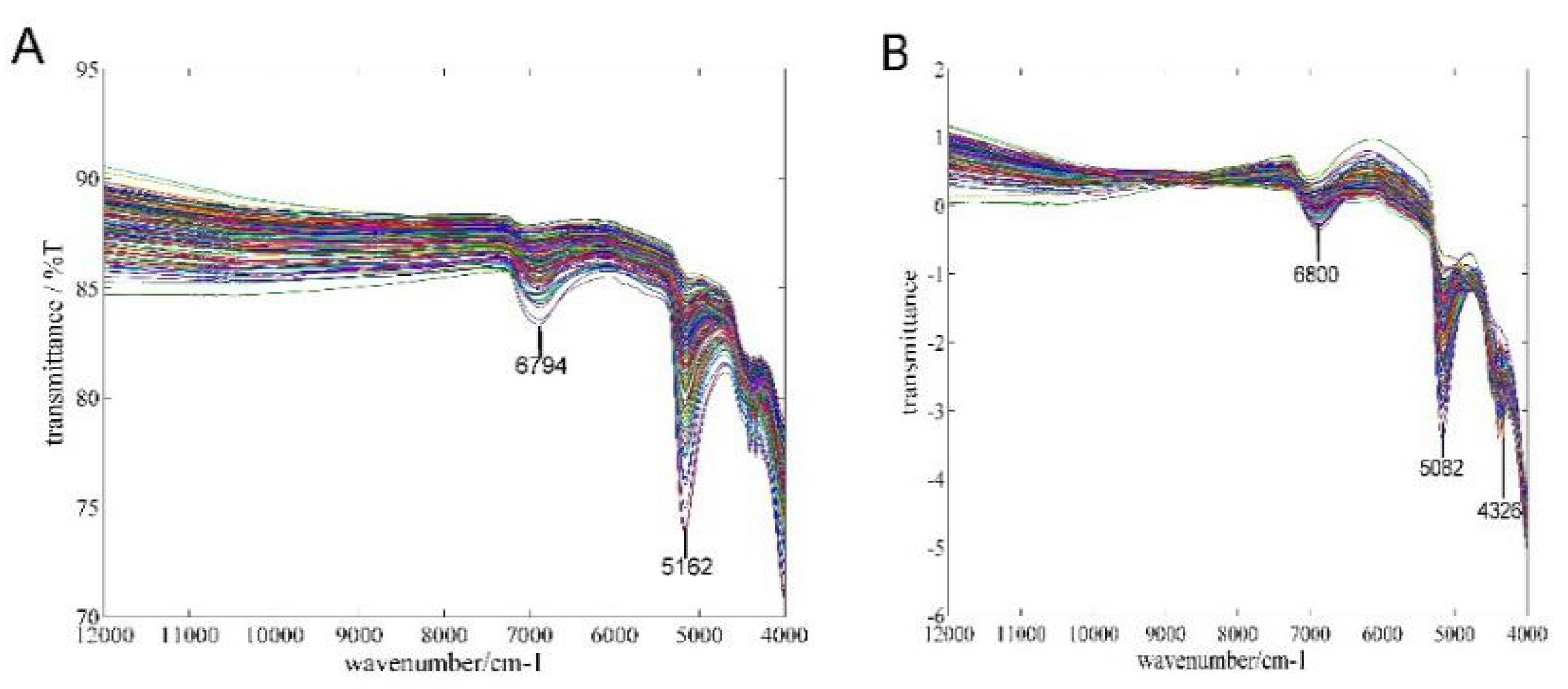
2.2. Spectral Acquisition from NIR Sensor
2.3. Spectral Preprocessing
| Method | RAW | MSC | SNV | SNV + DT | SG | SW | 1-Der | 2-Der |
|---|---|---|---|---|---|---|---|---|
| R | 0.8994 | 0.9325 | 0.9521 | 0.9444 | 0.8993 | 0.8991 | 0.9507 | 0.9512 |
| RMSECV | 0.1020 | 0.0845 | 0.0715 | 0.0769 | 0.1020 | 0.1020 | 0.0753 | 0.0771 |
3. The Proposed Method
3.1. SPA
- Step 1: In the initial iteration , a column vector is arbitrarily selected and denoted as , where is the starting position of the first selected variable. The location of the remaining columns are defined as , where .
- Step 2: Calculate the projection of the remaining column vectors with respect to the orthogonal vector space that consists of the selected vectors :where is the identity matrix and is the projection operator.
- Step 3: Extract the variable that has the maximum projection value , , and add it to the set of selected variables.
- Step 4: Let . If , return to Step 2 until .
3.2. EI
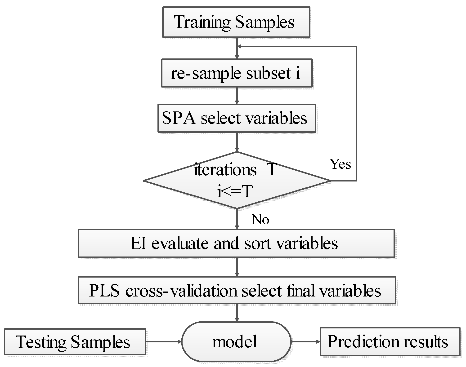
3.3. EBSPA
- Step 1: Set the number of iterations to . Use the bootstrap method to randomly select samples with replacement from the calibration set. In each iteration, the number of picked samples is the same as the size of the calibration set. The set of selected sample is .
- Step 2: Use SPA to select the variable subset from .
- Step 3: Let . If , then return to Step 1 to continue until the end of the iterations.
- Step 4: Take union set of the sets of the selected variables, remove the repeated variables, and obtain the ensemble set of variables .
- Step 5: Calculate the importance of each variable in according to Equation (2), and arrange the EI values in descending order.
- Step 6: Use the PLS cross-validation method to successively accumulate the sorted variables starting with maximum . When the minimum value of RMSECV is acquired, use the accumulated variables as the final selected set for EBSPA modeling.

4. Experiments and Discussion
4.1. Parameter Selection
4.1.1. Maximum Number of Selected Variables
| EBSPA-MLR | SPA-MLR | EBSPA-PLS | SPA-PLS | |||||
|---|---|---|---|---|---|---|---|---|
| R2 | RMSEP | R2 | RMSEP | R2 | RMSEP | R2 | RMSEP | |
| 10 | 0.9587 | 0.0582 | 0.9183 | 0.0818 | 0.9548 | 0.0608 | 0.9154 | 0.0824 |
| 15 | 0.9599 | 0.0573 | 0.9129 | 0.0871 | 0.9611 | 0.0565 | 0.9542 | 0.0612 |
| 20 | 0.9614 | 0.0563 | 0.9269 | 0.0788 | 0.9654 | 0.0534 | 0.9542 | 0.0612 |
| 25 | 0.9625 | 0.0555 | 0.9269 | 0.0788 | 0.9671 | 0.0521 | 0.9542 | 0.0612 |
| 30 | 0.9445 | 0.0672 | 0.9269 | 0.0788 | 0.9677 | 0.0516 | 0.9542 | 0.0612 |
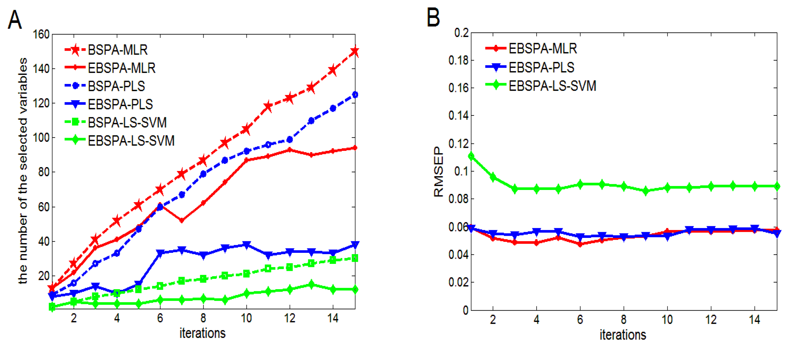
4.1.2. Number of Iterations

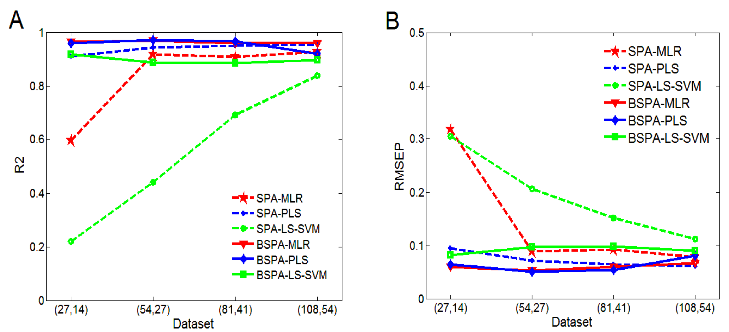
4.2. Performance Analysis of Small Sample Sizes

4.3. Performance Analysis of EI
| (27, 14) | (54, 27) | (81, 41) | (108, 54) | ||
|---|---|---|---|---|---|
| BSPA-MLR | R2 | 0.9645 | 0.9682 | 0.9591 | 0.9592 |
| RMSEP | 0.0599 | 0.0530 | 0.0594 | 0.0671 | |
| 117 | 116 | 107 | 105 | ||
| EBSPA-MLR | R2 | 0.9687 | 0.9767 | 0.9606 | 0.9614 |
| RMSEP | 0.0563 | 0.0455 | 0.0583 | 0.0563 | |
| 50 | 57 | 40 | 87 | ||
| BSPA-PLS | R2 | 0.9588 | 0.9716 | 0.9518 | 0.9192 |
| RMSEP | 0.0644 | 0.0501 | 0.0643 | 0.0806 | |
| 119 | 83 | 94 | 92 | ||
| EBSPA-PLS | R2 | 0.9704 | 0.9754 | 0.9665 | 0.9654 |
| RMSEP | 0.0547 | 0.0467 | 0.0538 | 0.0534 | |
| 20 | 28 | 36 | 38 | ||
| BSPA-LS-SVM | R2 | 0.9166 | 0.8883 | 0.8843 | 0.8972 |
| RMSEP | 0.0818 | 0.0973 | 0.0979 | 0.0904 | |
| 15 | 17 | 22 | 21 | ||
| EBSPA-LS-SVM | R2 | 0.9204 | 0.9510 | 0.8985 | 0.9024 |
| RMSEP | 0.0800 | 0.0633 | 0.0920 | 0.0882 | |
| 13 | 10 | 11 | 10 |
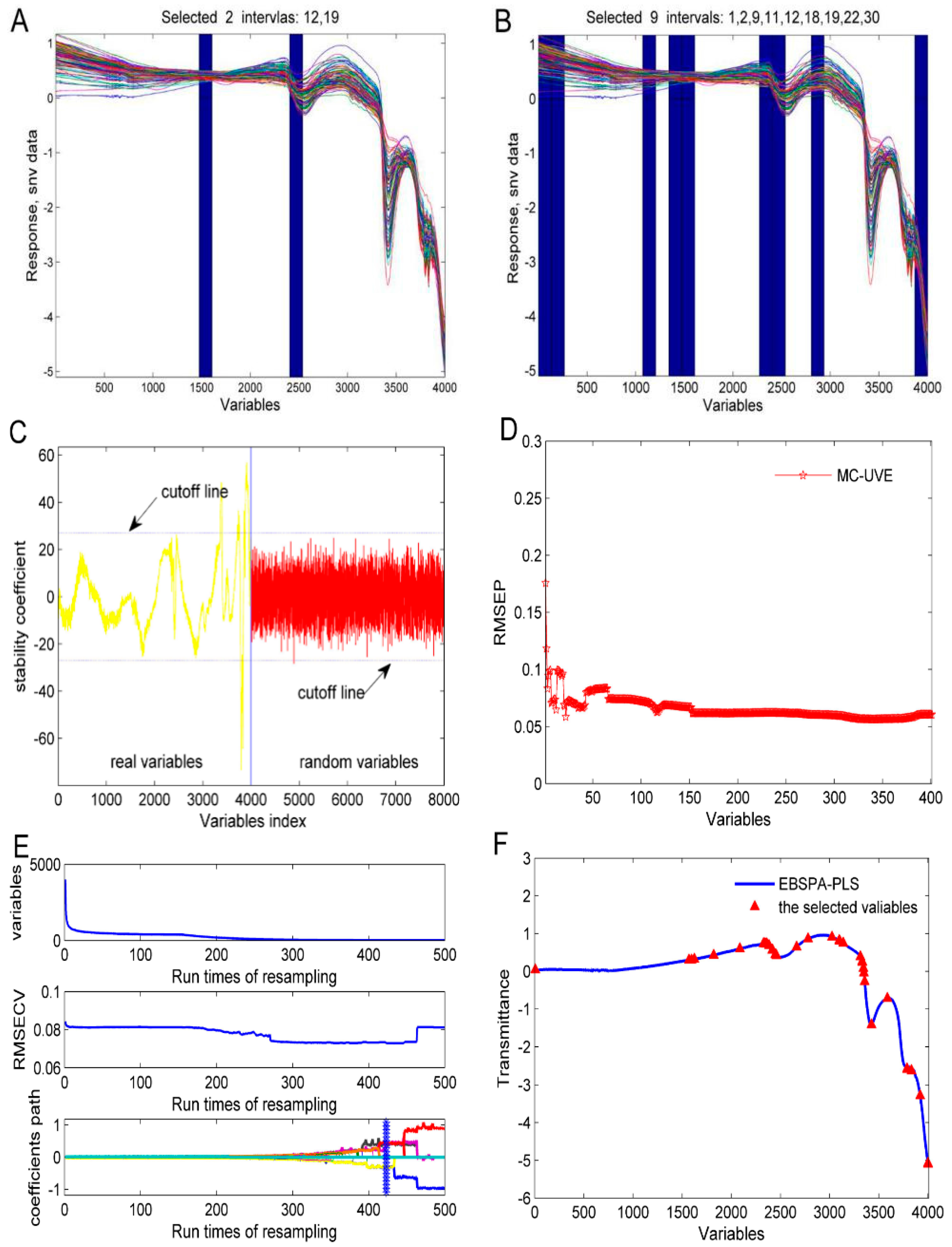
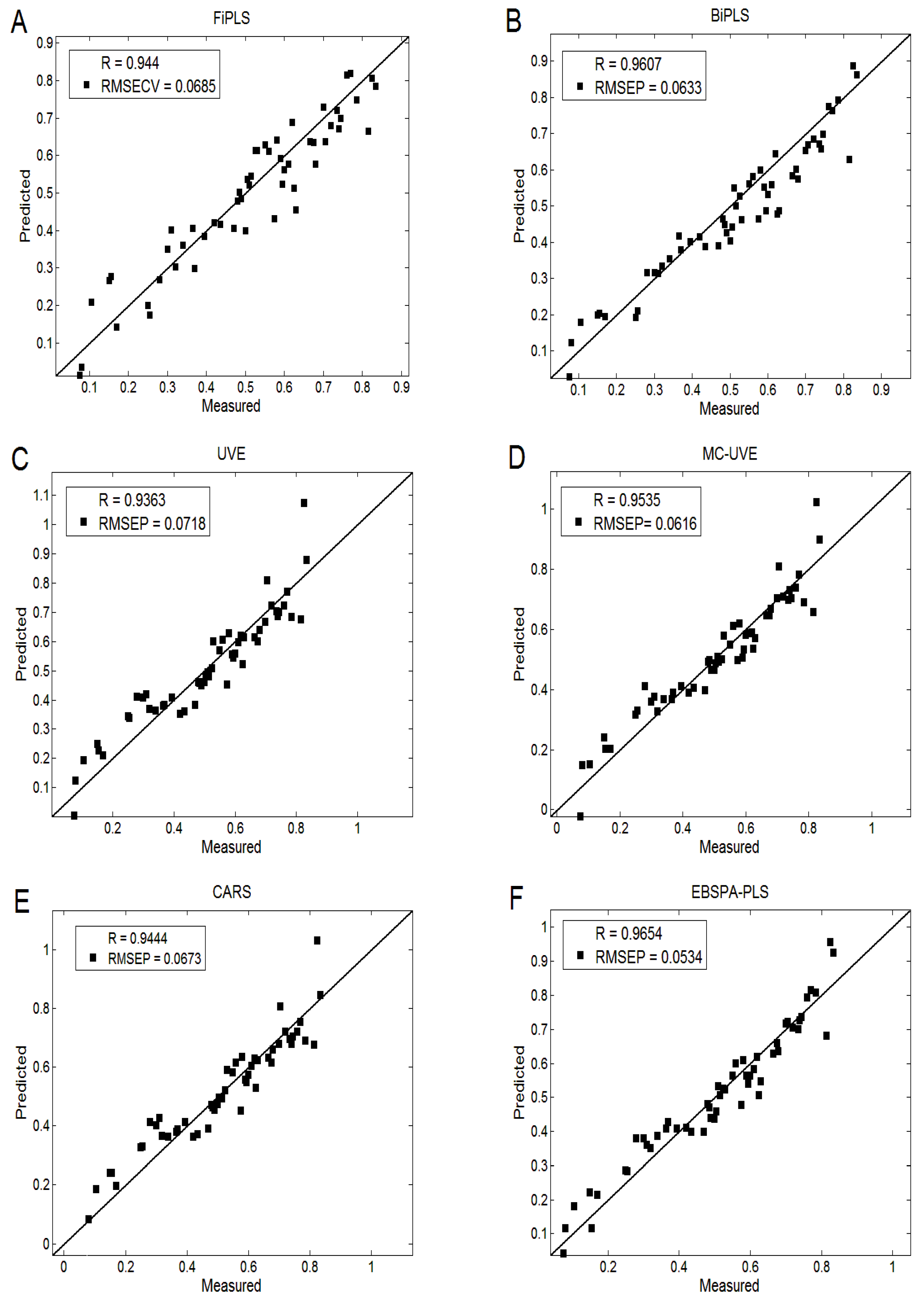
4.4. Comparison of Different Spectral Variable Selection Methods

| Method | Calibration Set | Validation Set | Variable Numbers | ||
|---|---|---|---|---|---|
| R1 | RMSEC | R2 | RMSEP | ||
| PLS | 0.9562 | 0.0707 | 0.9553 | 0.0605 | 4001 |
| FiPLS | 0.9696 | 0.0594 | 0.9440 | 0.0685 | 266 |
| BiPLS | 0.9711 | 0.0578 | 0.9607 | 0.0633 | 1199 |
| UVE | 0.9566 | 0.0704 | 0.9363 | 0.0718 | 214 |
| MC-UVE | 0.9536 | 0.0614 | 0.9535 | 0.0616 | 1571 |
| CARS | 0.9568 | 0.0702 | 0.9444 | 0.0673 | 29 |
| EBSPA-PLS | 0.9734 | 0.0523 | 0.9654 | 0.0534 | 38 |
5. Conclusions
Acknowledgments
Author Contributions
Conflicts of Interest
References
- Penza, M.; Cassano, G.; Aversa, P.; Antolini, F.; Cusano, A.; Cutolo, A.; Nicolais, L. Alcohol detection using carbon nanotubes acoustic and optical sensors. Appl. Phys. Lett. 2004, 85, 2379–2381. [Google Scholar] [CrossRef]
- Johansson, K.; Jönsson-Pettersson, G.; Gorton, L.; Marko-Varga, G.; Csöregi, E. A reagentless amperometric biosensor for alcohol detection in column liquid chromatography based on co-immobilized peroxidase and alcohol oxidase in carbon paste. J. Biotechnol. 1993, 31, 301–316. [Google Scholar] [CrossRef]
- Schiel, F.; Heinrich, C.; Neumeyer, V. Rhythm and formant features for automatic alcohol detection. In Proceedings of the INTERSPEECH 2010—11th Annual Conference of the International Speech Communication Association, Makuhari, Japan, 26–30 September 2010; pp. 458–461.
- Ridder, T.D.; Hendee, S.P.; Brown, C.D. Noninvasive alcohol testing using diffuse reflectance near-infrared spectroscopy. Appl. Spectrosc. 2005, 59, 181–189. [Google Scholar] [CrossRef] [PubMed]
- Castritius, S.; Kron, A.; Schäfer, T.; Rädle, M.; Harms, D. Determination of alcohol and extract concentration in beer samples using a combined method of near-infrared (NIR) spectroscopy and refractometry. J. Agric. Food. Chem. 2010, 58, 12634–12641. [Google Scholar] [CrossRef] [PubMed]
- Kim, S. Sea-Based Infrared Scene Interpretation by Background Type Classification and Coastal Region Detection for Small Target Detection. Sensors 2015, 15, 24487–24513. [Google Scholar] [CrossRef] [PubMed]
- Lim, J.; Kim, G.; Mo, C.; Kim, M.S. Design and Fabrication of a Real-Time Measurement System for the Capsaicinoid Content of Korean Red Pepper (Capsicum annuum L.) Powder by Visible and Near-Infrared Spectroscopy. Sensors 2015, 15, 27420–27435. [Google Scholar] [CrossRef] [PubMed]
- Sinelli, N.; Casiraghi, E.; Barzaghi, S.; Brambilla, A.; Giovanelli, G. Near infrared (NIR) spectroscopy as a tool for monitoring blueberry osmo-air dehydration process. Food. Res. Int. 2011, 44, 1427–1433. [Google Scholar] [CrossRef]
- Faassen, S.M.; Hitzmann, B. Fluorescence Spectroscopy and Chemometric Modeling for Bioprocess Monitoring. Sensors 2015, 15, 10271–10291. [Google Scholar] [CrossRef] [PubMed]
- Balabin, R.M.; Smirnov, S.V. Variable selection in near-infrared spectroscopy: Benchmarking of feature selection methods on biodiesel data. Anal. Chim. Acta. 2011, 692, 63–72. [Google Scholar] [CrossRef] [PubMed]
- Yong, H.; Xudong, S.; Hao, W. Spectral quantitative model optimization by modified successive projection algorithm. J. Jiangsu Univ. 2013, 34, 49–53. [Google Scholar]
- Guo, Z.M.; Huang, W.Q.; Peng, Y.K.; Wang, X.; Tang, X.Y. Adaptive Ant Colony Optimization Approach to Characteristic Wavelength Selection of NIR Spectroscopy. Chin. J. Anal. Chem. 2014, 42, 513–518. [Google Scholar]
- Mehmood, T.; Liland, K.H.; Snipen, L.; Sæbø, S. A review of variable selection methods in partial least squares regression. Chemometr. Intell. Lab. 2012, 118, 62–69. [Google Scholar] [CrossRef]
- Araújo, M.C.U.; Saldanha, T.C.B.; Galvão, R.K.H.; Yoneyama, T.; Chame, H.C.; Visani, V. The successive projections algorithm for variable selection in spectroscopic multicomponent analysis. Chemometr. Intell. Lab. 2001, 57, 65–73. [Google Scholar] [CrossRef]
- Du, G.; Cai, W.; Shao, X. A variable differential consensus method for improving the quantitative near-infrared spectroscopic analysis. Sci. China Chem. 2012, 55, 1946–1952. [Google Scholar] [CrossRef]
- Wu, D.; Ning, J.F.; Liu, X. Determination of anthocyanin content in grape skins using hyperspectral imaging technique and successive projections algorithm. Food Sci. 2014, 35, 57–61. [Google Scholar]
- Diniz, P.H.G.D.; Gomes, A.A.; Pistonesi, M.F.; Band, B.S.F.; de Araújo, M.C.U. Simultaneous Classification of Teas According to Their Varieties and Geographical Origins by Using NIR Spectroscopy and SPA-LDA. Food Anal. Methods 2014, 7, 1712–1718. [Google Scholar] [CrossRef]
- Zou, X.B.; Zhao, J.W.; Povey, M.J.; Holmes, M.; Mao, H. Variables selection methods in near-infrared spectroscopy. Anal. Chim. Acta 2010, 667, 14–32. [Google Scholar]
- Hong, Y.; Hong, T.; Dai, F.; Zhang, K.; Chen, H.; Li, Y. Successive projections algorithm for variable selection in nondestructive measurement of citrus total acidity. Trans. CSAE 2010, 26, 380–384. [Google Scholar]
- Liu, F.; He, Y. Application of successive projections algorithm for variable selection to determine organic acids of plum vinegar. Food Chem. 2009, 115, 1430–1436. [Google Scholar] [CrossRef]
- Wu, D.; Chen, X.; Zhu, X.; Guan, X.; Wu, G. Uninformative variable elimination for improvement of successive projections algorithm on spectral multivariable selection with different calibration algorithms for the rapid and non-destructive determination of protein content in dried laver. Anal. Methods 2011, 3, 1790–1796. [Google Scholar] [CrossRef]
- Soares, S.F.C.; Galvão, R.K.H.; Araújo, M.C.U.; Da Silva, E.C.; Pereira, C.F.; de Andrade, S.I.E.; Leite, F.C. A modification of the successive projections algorithm for spectral variable selection in the presence of unknown interferents. Anal. Chim. Acta 2011, 689, 22–28. [Google Scholar] [CrossRef] [PubMed]
- Soares, S.F.; Galvão, R.K.; Pontes, M.J.; Araújo, M.C. A new validation criterion for guiding the selection of variables by the successive projections algorithm in classification problems. J. Brazil. Chem. Soc. 2014, 25, 176–181. [Google Scholar] [CrossRef]
- Goodarzi, M.; Saeys, W.; de Araujo, M.C.U.; Galvão, R.K.H.; vander Heyden, Y. Binary classification of chalcone derivatives with LDA or KNN based on their antileishmanial activity and molecular descriptors selected using the successive projections algorithm feature-selection technique. Eur. J. Pharm. Sci. 2014, 51, 189–195. [Google Scholar] [CrossRef] [PubMed]
- Marreto, P.D.; Zimer, A.M.; Faria, R.C.; Mascaro, L.H.; Pereira, E.C.; Fragoso, W.D.; Lemos, S.G. Multivariate linear regression with variable selection by a successive projections algorithm applied to the analysis of anodic stripping voltammetry data. Electrochim. Acta 2014, 127, 68–78. [Google Scholar] [CrossRef]
- Xu, Z.B.; Si, X.B.; Li, C.; Chen, F. Study on the High-Speed Analysis of Coal Qualities by FT-NIR Method Based on Improved Successive Projections Algorithm. Adv. Mater. Res. 2015, 1094, 174–180. [Google Scholar] [CrossRef]
- Schapire, R.E. The strength of weak learnability. Mach. Learn. 1990, 5, 197–227. [Google Scholar] [CrossRef]
- Zou, X.; Zhao, J.; Li, Y. Selection of the efficient wavelength regions in FT-NIR spectroscopy for determination of SSC of “Fuji”apple based on BiPLS and FiPLS models. Vib. Spectrosc. 2007, 44, 220–227. [Google Scholar] [CrossRef]
- Centner, V.; Massart, D.L.; de Noord, O.E.; de Jong, S.; Vandeginste, B.M.; Sterna, C. Elimination of uninformative variables for multivariate calibration. Anal. Chem. 1996, 68, 3851–3858. [Google Scholar] [CrossRef] [PubMed]
- Gottardo, P.; de Marchi, M.; Cassandro, M.; Penasa, M. Technical note: Improving the accuracy of mid-infrared prediction models by selecting the most informative wavelengths. J. Dairy Sci. 2015, 98, 4168–4173. [Google Scholar] [CrossRef] [PubMed]
- Han, Q.J.; Wu, H.L.; Cai, C.B.; Xu, L.; Yu, R.Q. An ensemble of Monte Carlo uninformative variable elimination for wavelength selection. Anal. Chim. Acta 2008, 612, 121–125. [Google Scholar] [CrossRef] [PubMed]
- Lin, Z.; Pan, X.; Xu, B.; Zhang, J.; Shi, X.; Qiao, Y. Evaluating the reliability of spectral variables selected by subsampling methods. J. Chemometr. 2015, 29, 87–95. [Google Scholar] [CrossRef]
- Li, H.; Liang, Y.; Xu, Q.; Cao, D. Key wavelengths screening using competitive adaptive reweighted sampling method for multivariate calibration. Anal. Chim. Acta 2009, 648, 77–84. [Google Scholar] [CrossRef] [PubMed]
- Yun, Y.H.; Wang, W.T.; Deng, B.C.; Lai, G.B.; Liu, X.B.; Ren, D.B.; Xu, Q.S. Using variable combination population analysis for variable selection in multivariate calibration. Anal. Chim. Acta 2015, 862, 14–23. [Google Scholar] [CrossRef] [PubMed]
- Zhang, Z.Y. Determination of hesperidin in tangerine leaf by near-infrared spectroscopy with SPXY algorithm for sample subset partitioning and Monte Carlo cross validation. Spect. Anal. 2009, 29, 964–968. [Google Scholar]
- Dorado, M.P.; Pinzi, S.; de Haro, A.; Font, R.; Garcia-Olmo, J. Visible and NIR Spectroscopy to assess biodiesel quality: Determination of alcohol and glycerol traces. Fuel 2011, 90, 2321–2325. [Google Scholar] [CrossRef]
- Nordon, A.; Mills, A.; Burn, R.T.; Cusick, F.M.; Littlejohn, D. Comparison of non-invasive NIR and Raman spectrometries for determination of alcohol content of spirits. Anal. Chim. Acta 2005, 548, 148–158. [Google Scholar] [CrossRef]
- Moreira, E.D.T.; Pontes, M.J.C.; Galvão, R.K.H.; Araújo, M.C.U. Near infrared reflectance spectrometry classification of cigarettes using the successive projections algorithm for variable selection. Talanta 2009, 79, 1260–1264. [Google Scholar] [CrossRef] [PubMed]
- Zhang, S.Z.; Zhang, M.J. Wavelength selection from near infrared spectra by ensemble variable selection method. Comput. Appl. Chem. 2014, 31, 499–502. [Google Scholar]
- Fuchs, K.; Gertheiss, J.; Tutz, G. Nearest Neighbor Ensembles for Functional Data with Interpretable Feature Selection. Chemometr. Intell. Lab. 2015. [Google Scholar] [CrossRef]
- Zhang, H.L.; He, Y. Measurement of Soil Organic Matter and Available K Based on SPA-LS-SVM. Spect. Anal. 2014, 34, 1348–1351. [Google Scholar]
© 2016 by the authors; licensee MDPI, Basel, Switzerland. This article is an open access article distributed under the terms and conditions of the Creative Commons by Attribution (CC-BY) license (http://creativecommons.org/licenses/by/4.0/).
Share and Cite
Qu, F.; Ren, D.; Wang, J.; Zhang, Z.; Lu, N.; Meng, L. An Ensemble Successive Project Algorithm for Liquor Detection Using Near Infrared Sensor. Sensors 2016, 16, 89. https://doi.org/10.3390/s16010089
Qu F, Ren D, Wang J, Zhang Z, Lu N, Meng L. An Ensemble Successive Project Algorithm for Liquor Detection Using Near Infrared Sensor. Sensors. 2016; 16(1):89. https://doi.org/10.3390/s16010089
Chicago/Turabian StyleQu, Fangfang, Dong Ren, Jihua Wang, Zhong Zhang, Na Lu, and Lei Meng. 2016. "An Ensemble Successive Project Algorithm for Liquor Detection Using Near Infrared Sensor" Sensors 16, no. 1: 89. https://doi.org/10.3390/s16010089