
Generating Daily Synthetic Landsat Imagery by Combining Landsat and MODIS Data


Abstract
:1. Introduction
2. Methods
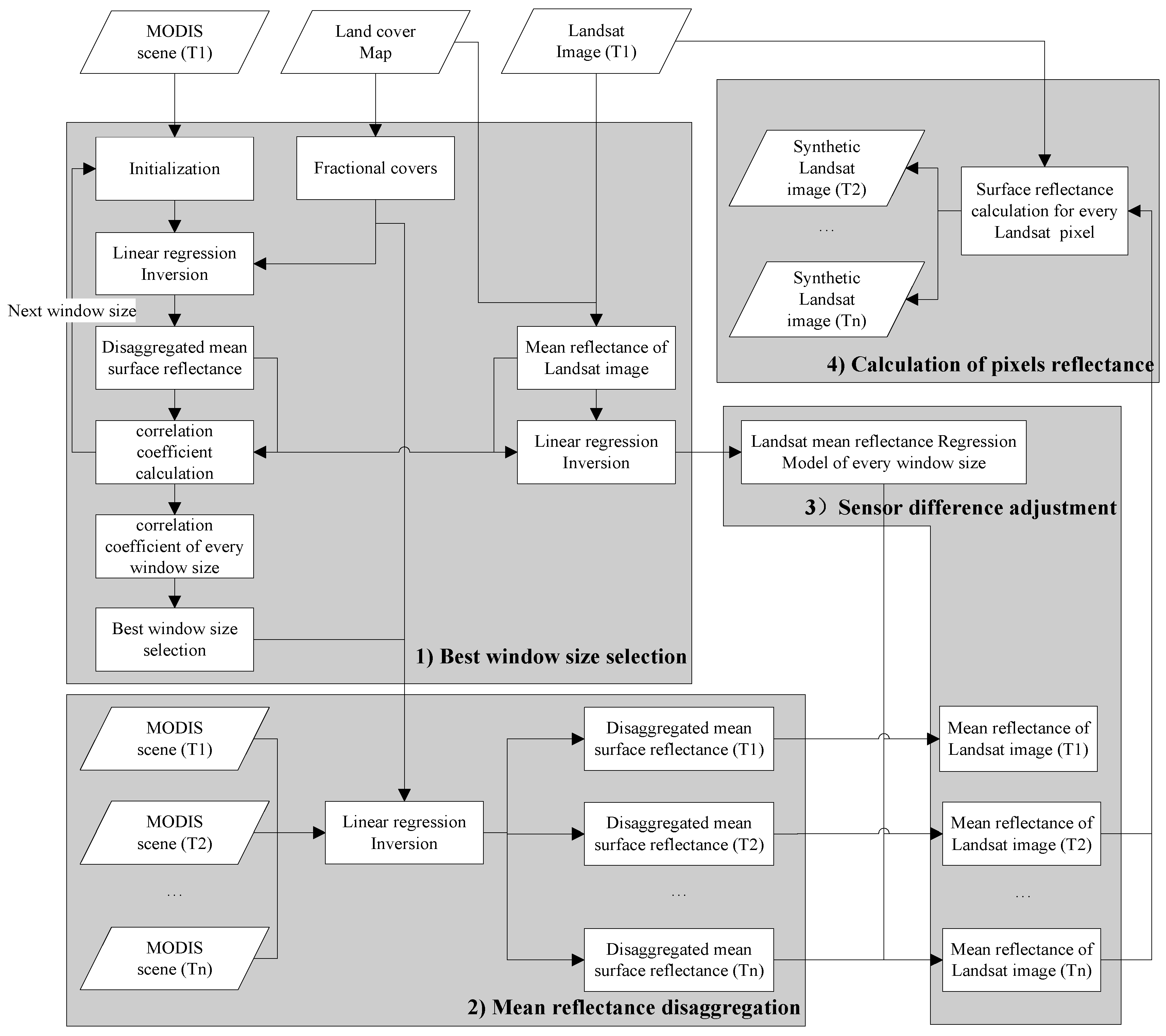
2.1. Method Inputs and Processing Steps

2.2. Selecting the Best Window Size
2.3. Disaggregating Mean Reflectance
2.4. Adjusting Sensor Difference
2.5. Calculating Pixels Reflectance and Method Outputs
3. Method Tests and Results
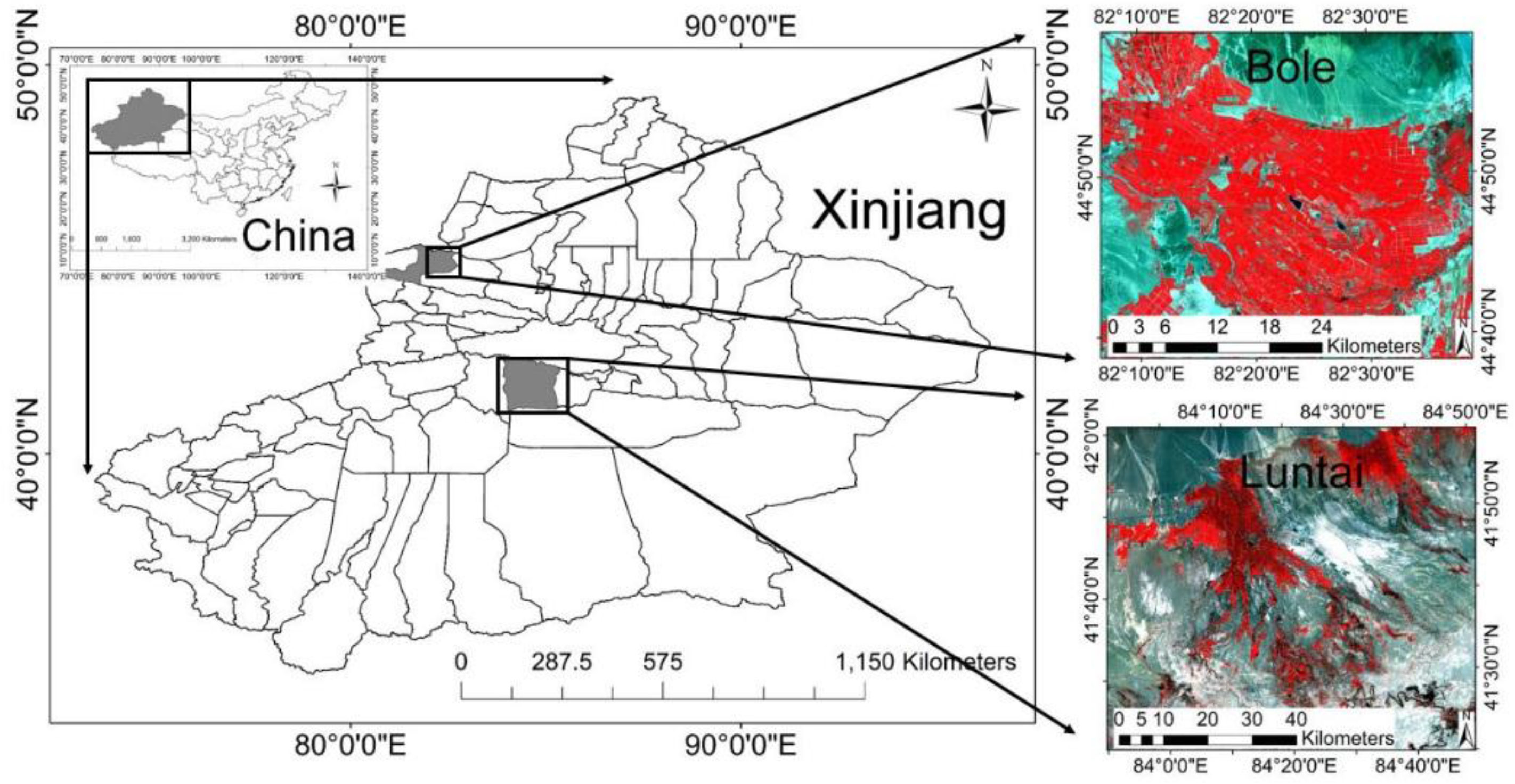
3.1. Study Area

3.2. Data and Pre-Processing
3.2.1. Landsat Data and Pre-Processing

| Study Area | Landsat-5 TM/ Landsat-8 OLI | MODIS | |||
|---|---|---|---|---|---|
| Acquisition Date | Path/Row | Usage | Acquisition Date | Usage | |
| Bole | 11 July 2011 | 146/29 | Reference Classification | 12 July 2011 | Mean reflectance estimation |
| 27 July 2011 | 146/29 | Validation | 28 July 2011 | ||
| 13 September 2011 | 146/29 | Validation | 14 September 2011 | ||
| Luntai | 4 September 2013 | 144/31 | Validation | 3 September 2013 | Mean reflectance estimation |
| 6 October 2013 | 144/31 | Reference Classification | 7 October 2013 | ||
| 22 October 2013 | 144/31 | Validation | 21 October 2013 | ||
3.2.2. MODIS Data and Pre-Processing
3.2.3. Land Cover Data
| Class | Reference Data | Prod. Acc. (%) | User Acc. (%) | ||||||
|---|---|---|---|---|---|---|---|---|---|
| Water | Forest | Grass | Shrub | Impervious | Cropland | Bare Land | |||
| Water | 1615 | 0 | 0 | 0 | 0 | 0 | 0 | 25.47 | 100 |
| Forest | 0 | 972 | 0 | 0 | 0 | 0 | 0 | 35.37 | 100 |
| Grass | 79 | 1775 | 349 | 372 | 824 | 541 | 0 | 27.35 | 8.86 |
| Shrub | 0 | 0 | 390 | 71 | 0 | 5 | 0 | 8.73 | 15.24 |
| Impervious | 700 | 0 | 0 | 0 | 2035 | 0 | 0 | 65.9 | 74.41 |
| Cropland | 425 | 0 | 470 | 370 | 200 | 25,928 | 0 | 96.03 | 94.65 |
| Bare land | 3522 | 1 | 67 | 0 | 29 | 525 | 5669 | 100 | 57.77 |
3.3. Results and Accuracy Assessment
3.3.1. Results of Landsat Mean Reflectance Regressing
| Bole | Best Window Size (MODIS pixels, 500 m) | |||||
|---|---|---|---|---|---|---|
| Class | Blue | Green | Red | NIR | SWIR1 | SWIR2 |
| Forest | 45 | 37 | 45 | 15 | 33 | 41 |
| Corn | 45 | 37 | 45 | 27 | 37 | 37 |
| Cotton | 15 | 23 | 19 | 35 | 45 | 19 |
| Desert | 35 | 35 | 39 | 45 | 39 | 39 |
| Bare land | 41 | 45 | 39 | 41 | 45 | 45 |
| Water | 31 | 23 | 25 | 35 | 37 | 43 |
| Building land | 35 | 37 | 37 | 45 | 43 | 13 |
| Other crops | 41 | 45 | 45 | 13 | 45 | 43 |
| Luntai | Best Window Size (MODIS pixels, 500 m) | |||||
| Class | Blue | Green | Red | NIR | SWIR1 | SWIR2 |
| Cotton | 71 | 73 | 73 | 37 | 33 | 21 |
| Water | 67 | 59 | 65 | 41 | 57 | 57 |
| Building land | 57 | 51 | 65 | 75 | 75 | 67 |
| Bare land | 15 | 19 | 75 | 75 | 19 | 39 |
| Desert | 63 | 39 | 33 | 37 | 49 | 13 |
| Corn | 73 | 73 | 73 | 73 | 71 | 73 |
| Bole: | ||||||||||||||||||
|---|---|---|---|---|---|---|---|---|---|---|---|---|---|---|---|---|---|---|
| Blue | Green | Red | NIR | SWIR1 | SWIR2 | |||||||||||||
| Class | R2 | a | b | R2 | a | b | R2 | a | b | R2 | a | b | R2 | a | b | R2 | a | b |
| Forest | 0.984 | 0.022 | 0.972 | 0.929 | 0.080 | 0.389 | 0.956 | 0.036 | 0.775 | 0.972 | 0.055 | 0.745 | 0.929 | 0.075 | 0.658 | 0.869 | 0.045 | 0.761 |
| Corn | 0.854 | 0.018 | 0.771 | 0.748 | 0.022 | 0.581 | 0.895 | 0.011 | 0.783 | 0.757 | 0.087 | 0.708 | 0.912 | 0.091 | 0.328 | 0.792 | 0.046 | 0.338 |
| Cotton | 0.490 | 0.035 | 0.205 | 0.487 | 0.023 | 0.700 | 0.593 | 0.031 | 0.519 | 0.939 | −0.039 | 1.021 | 0.821 | 0.025 | 0.787 | 0.584 | 0.041 | 0.511 |
| Desert | 0.966 | −0.021 | 1.364 | 0.994 | 0.010 | 0.974 | 0.996 | −0.005 | 1.003 | 0.996 | −0.027 | 1.043 | 0.990 | 0.003 | 0.907 | 0.996 | −0.028 | 1.015 |
| Bare land | 0.980 | 0.021 | 0.929 | 0.988 | 0.016 | 0.928 | 0.996 | 0.006 | 0.955 | 0.994 | 0.008 | 1.002 | 0.996 | −0.009 | 1.014 | 0.941 | −0.083 | 1.351 |
| Water | 0.914 | 0.027 | 0.931 | 0.962 | −0.017 | 1.233 | 0.986 | −0.002 | 1.046 | 0.984 | 0.060 | −0.120 | 0.543 | 0.022 | −0.073 | 0.642 | 0.015 | −0.035 |
| Building land | 0.806 | 0.037 | 0.861 | 0.953 | 0.001 | 0.982 | 0.958 | −0.019 | 1.045 | 0.984 | 0.028 | 0.858 | 0.918 | 0.012 | 0.552 | 0.824 | −0.053 | 0.925 |
| Other crops | 0.953 | 0.020 | 0.869 | 0.958 | −0.018 | 1.059 | 0.972 | −0.011 | 1.028 | 0.951 | 0.068 | 0.799 | 0.951 | −0.034 | 0.989 | 0.958 | 0.006 | 0.906 |
| Luntai: | ||||||||||||||||||
| Blue | Green | Red | NIR | SWIR1 | SWIR2 | |||||||||||||
| Class | R2 | a | b | R2 | a | b | R2 | a | b | R2 | a | b | R2 | a | b | R2 | a | b |
| Cotton | 0.910 | 0.007 | 0.831 | 0.824 | 0.014 | 0.763 | 0.841 | 0.032 | 0.678 | 0.699 | −0.018 | 1.102 | 0.691 | 0.056 | 0.685 | 0.555 | 0.082 | 0.423 |
| Water | 0.845 | 0.146 | −0.872 | 0.839 | 0.189 | −0.475 | 0.941 | 0.216 | −0.508 | 0.882 | −0.061 | 0.811 | 0.852 | −0.017 | 0.456 | 0.785 | 0.001 | 0.358 |
| Building land | 0.968 | 0.023 | 0.825 | 0.947 | 0.038 | 0.734 | 0.945 | 0.060 | 0.662 | 0.984 | 0.142 | 0.435 | 0.972 | 0.112 | 0.509 | 0.964 | 0.072 | 0.686 |
| Bare land | 0.968 | 0.029 | 0.902 | 0.990 | 0.005 | 1.013 | 0.990 | 0.056 | 0.836 | 0.994 | 0.048 | 0.873 | 0.996 | −0.007 | 1.022 | 0.994 | 0.006 | 0.991 |
| Desert | 0.962 | 0.056 | 0.766 | 0.937 | 0.128 | 0.541 | 0.916 | 0.146 | 0.556 | 0.964 | 0.149 | 0.586 | 0.750 | 0.248 | 0.351 | 0.676 | 0.121 | 0.660 |
| Corn | 0.867 | −0.011 | 1.108 | 0.755 | 0.011 | 0.792 | 0.752 | −0.001 | 0.910 | 0.870 | 0.078 | 0.826 | 0.627 | 0.147 | 0.297 | 0.585 | 0.072 | 0.483 |
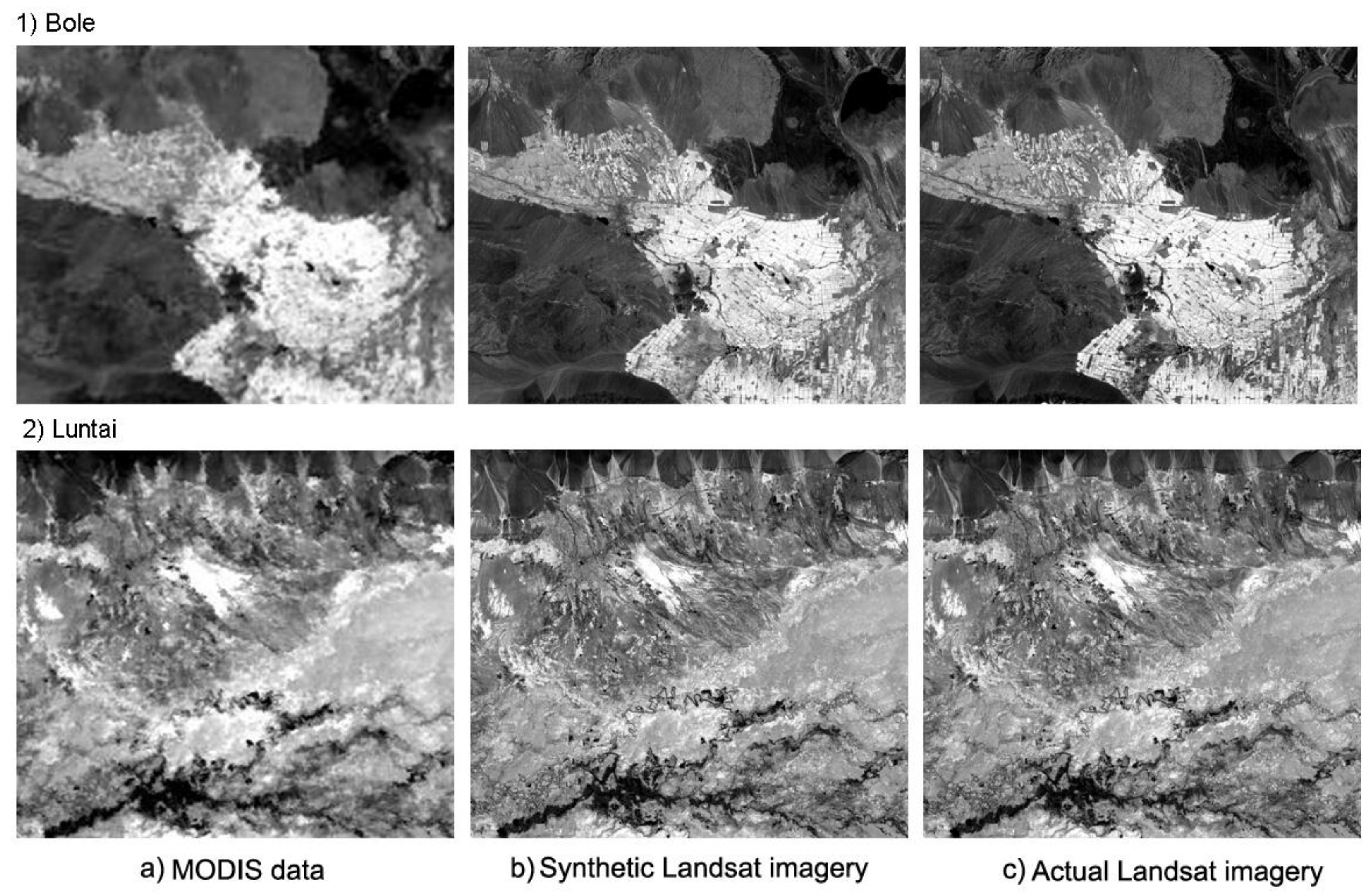
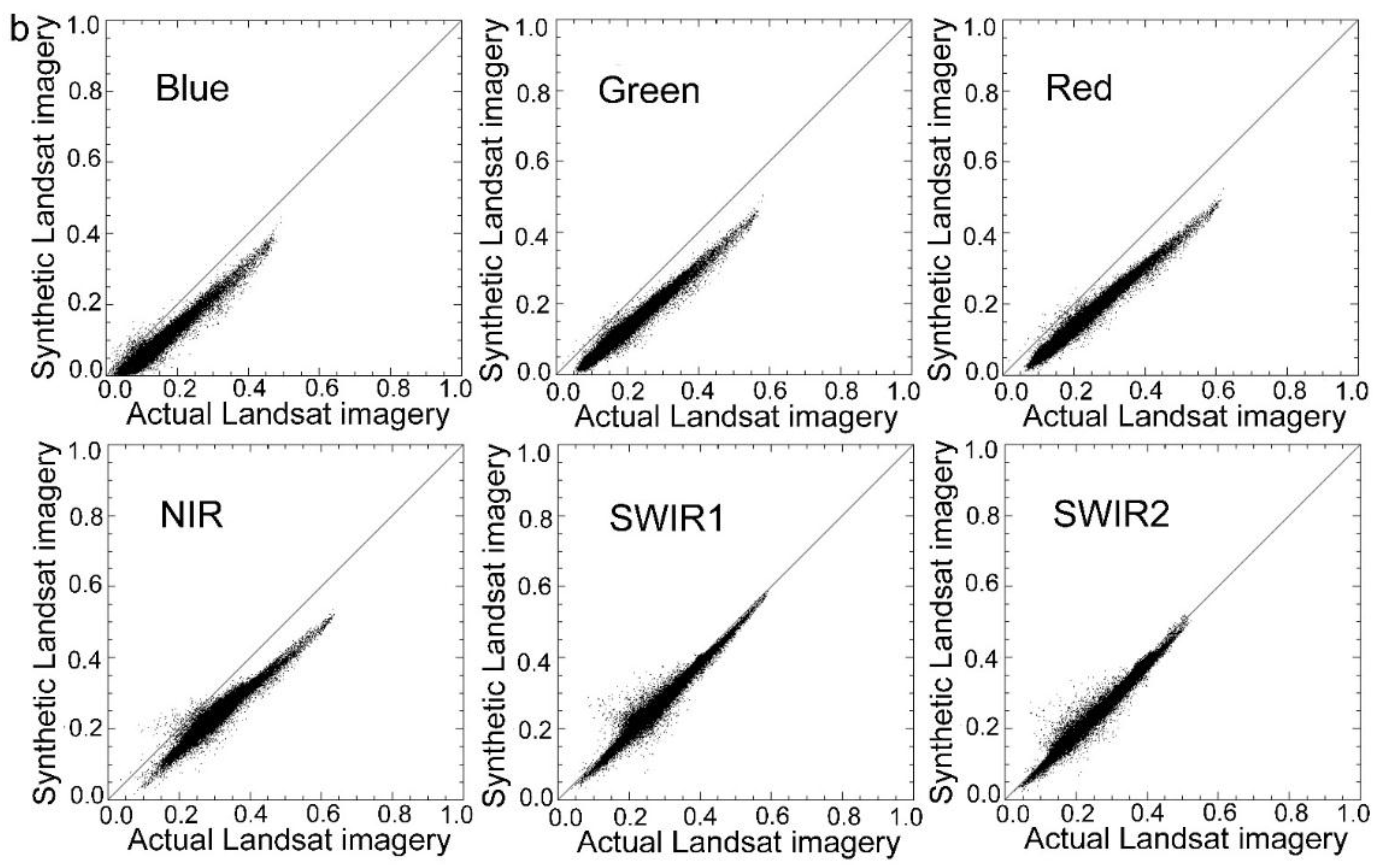
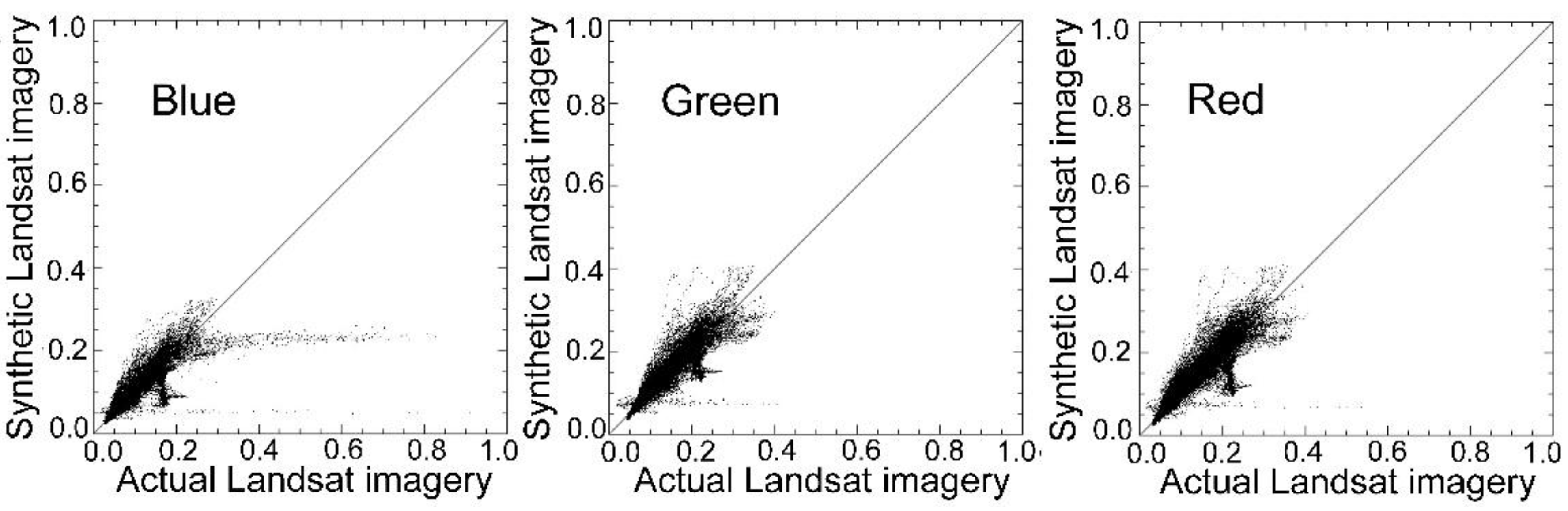
3.3.2. Results of Synthetic Landsat Image Generation

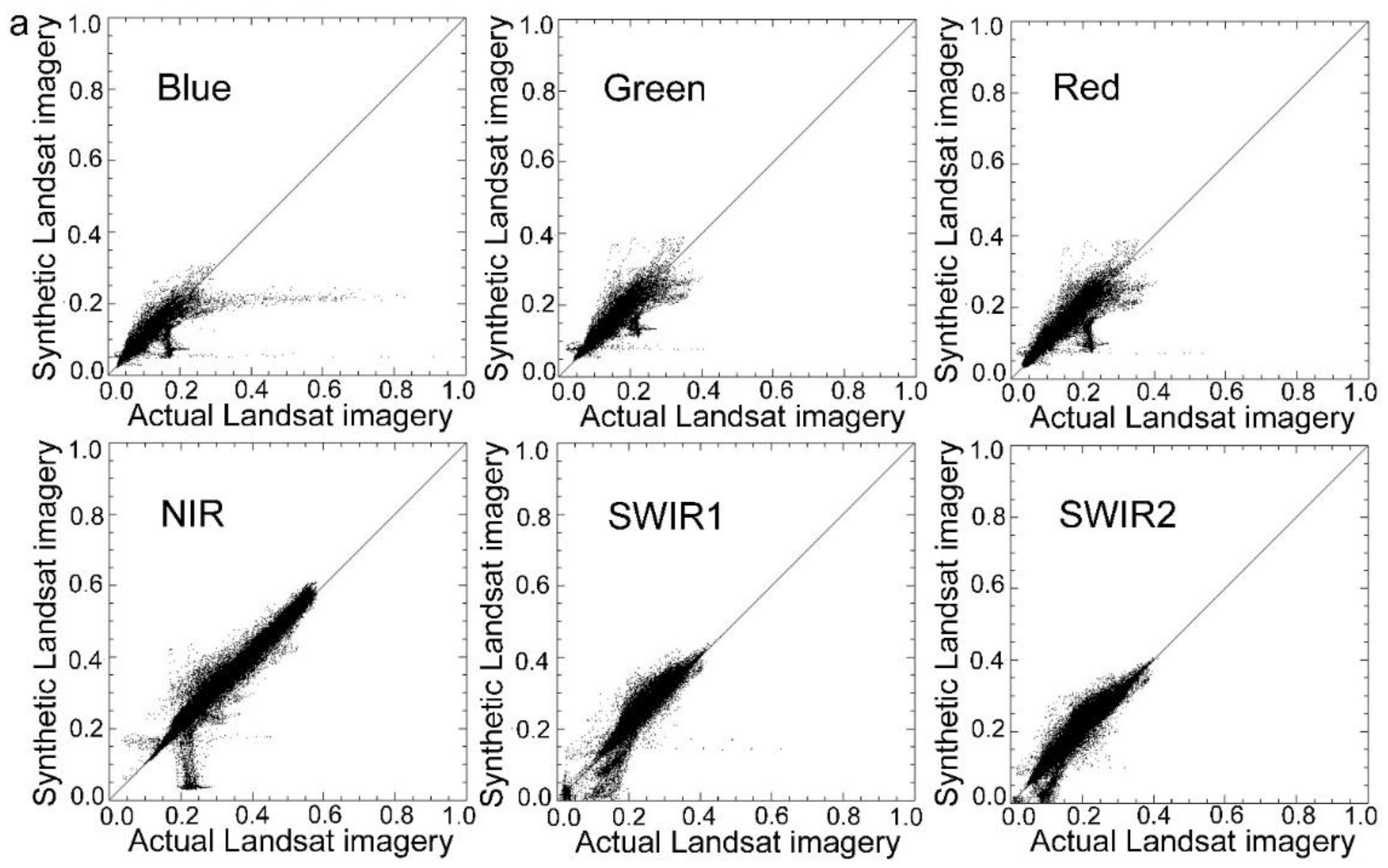
3.3.3. Accuracy Assessment
| Study Area | Bole | Luntai | ||||||||
|---|---|---|---|---|---|---|---|---|---|---|
| Date | 27 July 2011 | 4 September 2013 | ||||||||
| Parameters | R | Var | MAD | RMSE | Bias | R | Var | MAD | RMSE | Bias |
| Blue | 0.646 | 0.002 | 0.011 | 0.044 | −0.001 | 0.917 | <0.001 | 0.016 | 0.038 | 0.029 |
| Green | 0.909 | 0.003 | 0.012 | 0.023 | −0.003 | 0.925 | <0.001 | 0.018 | 0.031 | 0.018 |
| Red | 0.918 | 0.004 | 0.015 | 0.027 | −0.003 | 0.930 | <0.001 | 0.020 | 0.032 | 0.015 |
| NIR | 0.961 | 0.016 | 0.020 | 0.036 | −0.006 | 0.856 | <0.001 | 0.023 | 0.034 | 0.014 |
| SWIR1 | 0.932 | 0.007 | 0.018 | 0.031 | −0.007 | 0.893 | <0.001 | 0.021 | 0.033 | 0.013 |
| SWIR2 | 0.946 | 0.010 | 0.020 | 0.032 | −0.005 | 0.909 | <0.001 | 0.021 | 0.033 | 0.012 |
| Date | 13 September 2011 | 22 October 2013 | ||||||||
| Parameters | R | Var | MAD | RMSE | Bias | R | Var | MAD | RMSE | Bias |
| Blue | 0.735 | 0.002 | 0.012 | 0.041 | 0.004 | 0.980 | <0.001 | 0.006 | 0.010 | 0.001 |
| Green | 0.902 | <0.001 | 0.015 | 0.026 | 0.005 | 0.985 | <0.001 | 0.007 | 0.014 | 0.008 |
| Red | 0.904 | <0.001 | 0.017 | 0.030 | 0.004 | 0.986 | <0.001 | 0.008 | 0.017 | 0.011 |
| NIR | 0.839 | 0.003 | 0.034 | 0.051 | 0.001 | 0.968 | <0.001 | 0.008 | 0.017 | 0.009 |
| SWIR1 | 0.868 | <0.001 | 0.022 | 0.034 | 0.004 | 0.979 | <0.001 | 0.009 | 0.018 | 0.010 |
| SWIR2 | 0.903 | <0.001 | 0.023 | 0.037 | 0.010 | 0.986 | <0.001 | 0.009 | 0.019 | 0.011 |

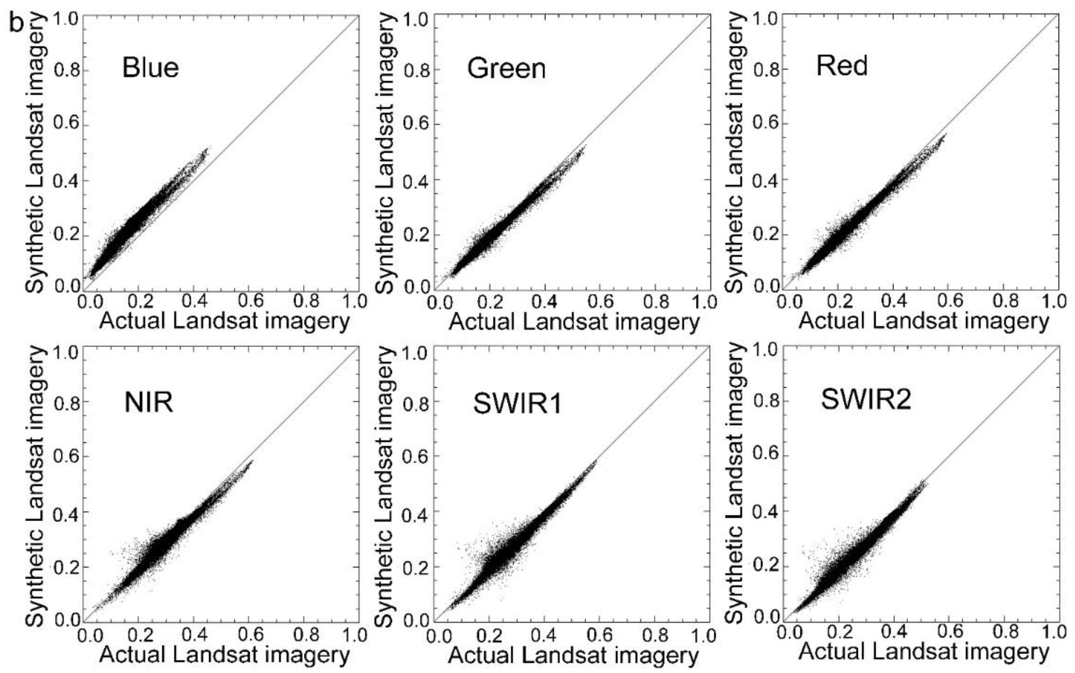
4. Discussion
4.1. Comparison to STDFA
| Study Area | Bole | Luntai | ||||||||
|---|---|---|---|---|---|---|---|---|---|---|
| Date | 27 July 2011 | 4 September 2013 | ||||||||
| Parameters | R | Var | MAD | RMSE | Bias | R | Var | MAD | RMSE | Bias |
| Blue | 0.654 | 0.002 | 0.010 | 0.043 | −0.001 | 0.912 | <0.001 | 0.018 | 0.035 | 0.025 |
| Green | 0.919 | <0.001 | 0.011 | 0.021 | −0.002 | 0.922 | <0.001 | 0.018 | 0.030 | 0.016 |
| Red | 0.930 | 0.001 | 0.013 | 0.024 | −0.002 | 0.930 | <0.001 | 0.020 | 0.031 | 0.014 |
| NIR | 0.961 | 0.001 | 0.020 | 0.035 | −0.006 | 0.864 | <0.001 | 0.022 | 0.035 | 0.016 |
| SWIR1 | 0.894 | 0.001 | 0.019 | 0.037 | −0.003 | 0.872 | <0.001 | 0.022 | 0.038 | 0.020 |
| SWIR2 | 0.889 | 0.002 | 0.024 | 0.047 | 0.001 | 0.892 | <0.001 | 0.024 | 0.038 | 0.018 |
| Date | 27 July 2011 | 22 October 2013 | ||||||||
| Parameters | R | Var | MAD | RMSE | Bias | R | Var | MAD | RMSE | Bias |
| Blue | 0.735 | 0.002 | 0.013 | 0.041 | 0.002 | 0.968 | <0.001 | 0.010 | 0.060 | 0.058 |
| Green | 0.907 | <0.001 | 0.016 | 0.026 | 0.004 | 0.974 | <0.001 | 0.011 | 0.070 | 0.068 |
| Red | 0.899 | <0.001 | 0.019 | 0.030 | 0.001 | 0.977 | <0.001 | 0.012 | 0.071 | 0.069 |
| NIR | 0.769 | 0.004 | 0.041 | 0.062 | 0.002 | 0.956 | <0.001 | 0.011 | 0.069 | 0.066 |
| SWIR1 | 0.863 | 0.001 | 0.023 | 0.035 | −0.001 | 0.978 | <0.001 | 0.010 | 0.020 | 0.010 |
| SWIR2 | 0.894 | 0.001 | 0.025 | 0.038 | 0.002 | 0.956 | <0.001 | 0.007 | 0.026 | 0.025 |


4.2. Improvement
| Parameters | STDFA | Adaptive Window Size Selection | Sensor Adjustment | Total |
|---|---|---|---|---|
| R | 0.9557 | +0.0116 | +0.0003 | 0.9676 |
| Variance | 0.0003 | −0.0001 | 0.0000 | 0.0002 |
| MAD | 0.0113 | −0.0027 | −0.0003 | 0.0083 |
| RMSE | 0.0688 | −0.0502 | −0.0013 | 0.0173 |
| Bias | 0.0664 | −0.0548 | −0.0021 | 0.0095 |
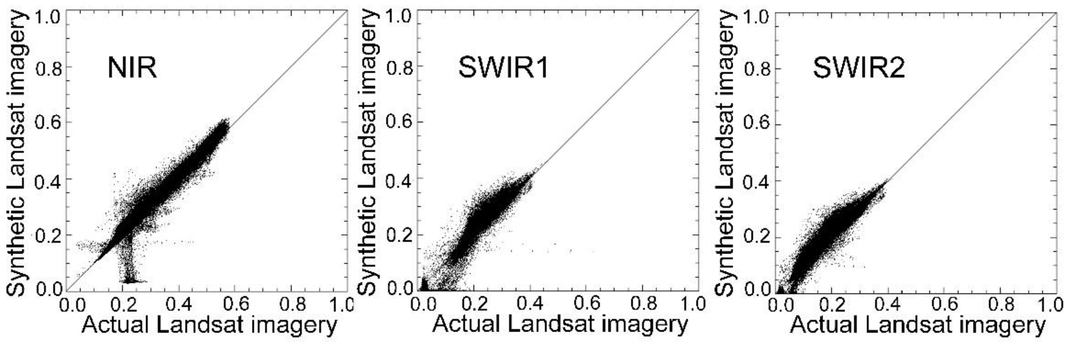
4.3. Landsat and MODIS Fusion Using FROM–GLC Data
| Parameters | R | Variance | MAD | RMSE | Bias |
|---|---|---|---|---|---|
| Blue | 0.661 | 0.002 | 0.011 | 0.043 | −0.003 |
| Green | 0.917 | 0.000 | 0.012 | 0.022 | −0.003 |
| Red | 0.924 | 0.001 | 0.014 | 0.026 | −0.004 |
| NIR | 0.961 | 0.001 | 0.021 | 0.036 | −0.007 |
| SWIR1 | 0.936 | 0.001 | 0.017 | 0.030 | −0.010 |
| SWIR2 | 0.956 | 0.001 | 0.019 | 0.029 | −0.008 |

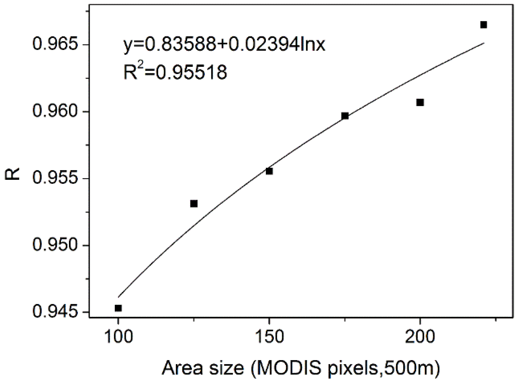
4.4. Influence of the Image Extents

4.5. Comparison of Actual NDVI and NDVI Calculated Using Synthetic Data
| NDVI Generated by MSTDFA | NDVI Generated by STDFA | |
|---|---|---|
| R | 0.970 | 0.949 |
| Variance | 0.006 | 0.010 |
| MAD | 0.043 | 0.074 |
| RMSE | 0.086 | 0.125 |
| Bias | 0.037 | 0.073 |
4.6. Limitations of the Method
| R | Variance | MAD | RMSE | Bias | |
|---|---|---|---|---|---|
| Blue | 0.974 | <0.001 | 0.005 | 0.011 | −0.001 |
| Green | 0.989 | <0.001 | 0.006 | 0.010 | −0.002 |
| Red | 0.988 | <0.001 | 0.008 | 0.012 | −0.001 |
| NIR | 0.997 | <0.001 | 0.009 | 0.014 | −0.004 |
| SWIR1 | 0.990 | <0.001 | 0.010 | 0.017 | −0.005 |
| SWIR2 | 0.986 | <0.001 | 0.012 | 0.019 | −0.004 |
5. Conclusions
- (1)
- The adaptive window size and moving step selection method can select the best window size for disaggregation of coarse pixels. The disaggregated mean coarse reflectance had a strong linear relationship with the Landsat mean reflectance.
- (2)
- MSTDFA had higher accuracy than STDFA but was more easily influenced by land cover change. Land cover data such as that of FROM-GLC can be used in MSTDFA. Synthetic Landsat images with high similarity to actual Landsat images with a correlation coefficient R of 0.96 can be generated.
- (3)
- Land cover class change had a very important influence in MSTDFA, which can lead to a reduction in the correlation coefficient R of 0.32 in the blue band.
- (4)
- MSTDFA can be applied in 250 m 16-day MODIS MOD13Q1 products and Landsat NDVI data. A synthetic NDVI image with very high similarity to the actual NDVI observation with a high correlation coefficient R of 0.97 can be generated.
Acknowledgments
Author Contributions
Conflicts of Interest
Abbreviations
| MSTDFA | Modified Spatial and Temporal Data Fusion Approach |
| MODIS | Moderate Resolution Imaging Spectroradiometer |
| STDFA | Spatial and Temporal Data Fusion Approach |
| NDVI | Normalized Different Vegetation Index |
| AVHRR | Advanced Very High Resolution Radiometer |
| SPOT | Systeme Pour l’Observation de la Terre |
| VGT | Vegetation |
| TM | Thematic Mapper |
| ETM+ | Enhanced Thematic Mapper Plus |
| OLI | Operational Land Imager |
| STARFM | Spatial and Temporal Adaptive Reflectance Fusion Model |
| STAARCH | Spatial Temporal Adaptive Algorithm for mapping Reflectance Change |
| ESTARFM | Enhanced Spatial and Temporal Adaptive Reflectance Fusion Model |
| FROM-GLC | Finer Resolution Observation and Monitoring of Global Land Cover |
| HJ | Huanjing |
| CCD | Charge Coupled Device |
| GF-1 | Gaofen satellite No. 1 |
| WFV | Wide Field of View camera |
| USGS | United States Geological Survey |
| FLAASH | Fast Line-of-Sight Atmospheric Analysis of Spectral Hypercubes |
| GCPs | Ground Control Points |
| MRT | MODIS Reprojection Tool |
| NLCD | National Land Cover Database |
| NIR | Near Infrared Reflection |
| SWIR | shortwave infrared |
| MAD | Mean Absolute Difference |
| RMSE | Root Mean Square Error |
References
- Fensholt, R.; Anyamba, A.; Huber, S.; Proud, S.R.; Tucker, C.J.; Small, J.; Pak, E.; Rasmussen, M.O.; Sandholt, I.; Shisanya, C. Analysing the advantages of high temporal resolution geostationary MSG SEVIRI data compared to Polar Operational Environmental Satellite data for land surface monitoring in Africa. Int. J. Appl. Earth Obs. Geoinf. 2011, 13, 721–729. [Google Scholar] [CrossRef]
- Politi, E.; Cutler, M.E.J.; Rowan, J.S. Using the NOAA advanced very high resolution radiometer to characterise temporal and spatial trends in water temperature of large European lakes. Remote Sens. Environ. 2012, 126, 1–11. [Google Scholar] [CrossRef] [Green Version]
- Maisongrande, P.; Duchemin, B.; Dedieu, G. VEGETATION/SPOT: An operational mission for the Earth monitoring; presentation of new standard products. Int. J. Remote Sens. 2004, 25, 9–14. [Google Scholar] [CrossRef]
- Salomonson, V.V.; Barnes, W.L.; Maymon, P.W.; Montgomery, H.E.; Ostrow, H. MODIS: Advanced facility instrument for studies of the earth as a system. IEEE Trans. Geosci. Remote Sens. 1992, 27, 145–153. [Google Scholar] [CrossRef]
- Zhang, X.; Sun, R.; Zhang, B.; Tong, Q.X. Land cover classification of the North China Plain using MODIS EVI time series. ISPRS J. Photogramm. Remote Sens. 2008, 63, 476–484. [Google Scholar] [CrossRef]
- Carrão, H.; Gonçalves, P.; Caetano, M. Contribution of multispectral and multitemporal information from MODIS images to land cover classification. Remote Sens. Environ. 2008, 112, 986–997. [Google Scholar] [CrossRef]
- Thenkabail, P.S.; Schull, M.; Turral, H. Ganges and Indus river basin land use/land cover (LULC) and irrigated area mapping using continuous streams of MODIS data. Remote Sens. Environ. 2008, 95, 317–341. [Google Scholar] [CrossRef]
- Kim, Y.; Kimball, J.S.; Didan, K.; Henebry, G.M. Response of vegetation growth and productivity to spring climate indicators in the conterminous United States derived from satellite remote sensing data fusion. Agric. Forest Meteorol. 2014, 194, 132–143. [Google Scholar] [CrossRef]
- Estel, S.; Kuemmerle, T.; Alcántara, C.; Levers, C.; Prishchepov, A.; Hostert, P. Mapping farmland abandonment and recultivation across Europe using MODIS NDVI time series. Remote Sens. Environ. 2015, 163, 312–325. [Google Scholar] [CrossRef]
- Eckert, S.; Hüsler, F.; Liniger, H.; Hodel, E. Trend analysis of MODIS NDVI time series for detecting land degradation and regeneration in Mongolia. J. Arid Environ. 2015, 113, 16–28. [Google Scholar] [CrossRef]
- Chen, C.F.; Son, N.T.; Chang, L.Y. Monitoring of rice cropping intensity in the upper Mekong Delta, Vietnam using time-series MODIS data. Adv. Space Res. 2012, 49, 292–301. [Google Scholar] [CrossRef]
- Zhang, J.; Feng, L.; Yao, F. Improved maize cultivated area estimation over a large scale combining MODIS–EVI time series data and crop phenological information. ISPRS J. Photogramm. Remote Sens. 2014, 94, 102–113. [Google Scholar] [CrossRef]
- Huesca, M.; Litago, J.; Merino-de-Miguel, S.; Cicuendez-López-Ocaña, V.; Palacios-Orueta, A. Modeling and forecasting MODIS-based Fire Potential Index on a pixel basis using time series models. Int. J. Appl. Earth Obs. Geoinf. 2014, 26, 363–376. [Google Scholar] [CrossRef]
- Sakamoto, T.; Nguyen, N.V.; Kotera, A.; Ohno, H.; Ishitsuka, N.; Yokozawa, M. Detecting temporal changes in the extent of annual flooding within the Cambodia and the Vietnamese Mekong Delta from MODIS time-series imagery. Remote Sens. Environ. 2007, 109, 295–313. [Google Scholar] [CrossRef]
- Sulla-Menashe, D.; Kennedy, R.E.; Yang, Z.; Braaten, J.; Krankina, O.N.; Friedl, M.A. Detecting forest disturbance in the Pacific Northwest from MODIS time series using temporal segmentation. Remote Sens. Environ. 2014, 151, 114–123. [Google Scholar] [CrossRef]
- Cao, R.; Chen, J.; Shen, M.; Tang, Y. An improved logistic method for detecting spring vegetation phenology in grasslands from MODIS EVI time-series data. Agric. Forest Meteorol. 2015, 200, 9–20. [Google Scholar] [CrossRef]
- Gong, P.; Wang, J.; Yu, L.; Zhao, Y.C.; Zhao, Y.Y.; Liang, L.; Niu, Z.; Huang, X.; Fu, H.; Liu, S.; et al. Finer resolution observation and monitoring of global land cover: First mapping results with Landsat TM and ETM+ data. Int. J. Remote Sens. 2013, 34, 2607–2654. [Google Scholar] [CrossRef]
- Jia, K.; Liang, S.L.; Zhang, N.; Wei, X.; Gu, X.; Zhao, X.; Yao, Y.; Xie, X. Land cover classification of finer resolution remote sensing data integrating temporal features from time series coarser resolution data. ISPRS J. Photogramm. Remote Sens. 2014, 93, 49–55. [Google Scholar] [CrossRef]
- Fu, D.J.; Chen, B.Z.; Zhang, H.F.; Wang, J.; Black, T.A.; Amiro, B.D.; Bohrer, G.; Bolstad, P.; Coulter, R.; Rahman, A.F.; et al. Estimating landscape net ecosystem exchange at high spatial-temporal resolution based on Landsat data, an improved upscaling model framework, and eddy covariance flux measurements. Remote Sens. Environ. 2014, 141, 90–104. [Google Scholar] [CrossRef]
- Jeniffer, K.; Su, Z.B.; Woldai, T.; Maathuis, B. Estimation of spatial-temporal rainfall distribution using remote sensing techniques: A case study of Makanya catchment, Tanzania. Int. J. Appl. Earth Obs. Geoinf. 2010, 12, S90–S99. [Google Scholar] [CrossRef]
- Du, P.J.; Liu, S.C.; Xia, J.S.; Zhao, Y. Information fusion techniques for change detection from multi-temporal remote sensing images. Inf. Fusion 2013, 14, 19–27. [Google Scholar] [CrossRef]
- Leckie, D. Advances in remote sensing technologies for forest surveys and management. Can. J. Forest Res. 1990, 21, 464–483. [Google Scholar] [CrossRef]
- Gao, F.; Masek, J.; Schwaller, M.; Hall, F. On the blending of the Landsat and MODIS surface reflectance: Predicting daily Landsat surface reflectance. IEEE Trans. Geosci. Remote Sens. 2006, 44, 2207–2218. [Google Scholar]
- Roy, D.P.; Ju, J.C.; Lewis, P.; Schaaf, C.; Gao, F.; Hansen, M.; Lindquist, E. Multi-temporal MODIS–Landsat data fusion for relative radiometric normalization, gap filling, and prediction of Landsat data. Remote Sens. Environ. 2008, 112, 3112–3130. [Google Scholar] [CrossRef]
- Hilker, T.; Wulder, M.A.; Coops, N.C.; Linke, J.; McDermid, G.; Masek, J.G.; Gao, F.; White, J.C. A new data fusion model for high spatial- and temporal- resolution mapping of forest disturbance based on Landsat and MODIS. Remote Sens. Environ. 2009, 113, 1613–1627. [Google Scholar] [CrossRef]
- Liu, H.; Weng, Q.H. Enhancing temporal resolution of satellite imagery for public health studies: A case study of West Nile Virus outbreak in Los Angeles in 2007. Remote Sens. Environ. 2012, 117, 57–71. [Google Scholar] [CrossRef]
- Walker, J.J.; Beurs, K.M.; Wynne, R.H.; Gao, F. Evaluation of Landsat and MODIS data fusion products for analysis of dry land forest phonology. Remote Sens. Environ. 2012, 117, 381–393. [Google Scholar] [CrossRef]
- Weng, Q.H.; Fua, P.; Gao, F. Generating daily land surface temperature at Landsat resolution by fusing Landsat and MODIS data. Remote Sens. Environ. 2014, 145, 55–67. [Google Scholar] [CrossRef]
- Schmidt, M.; Lucas, R.; Bunting, P.; Verbesselt, J.; Armston, J. Multi-resolution time series imagery for forest disturbance and regrowth monitoring in Queensland, Australia. Remote Sens. Environ. 2015, 158, 156–168. [Google Scholar] [CrossRef] [Green Version]
- Zhu, X.L.; Chen, J.; Gao, F.; Chen, X.; Masek, J.G. An enhanced spatial and temporal adaptive reflectance fusion model for complex heterogeneous regions. Remote Sens. Environ. 2010, 114, 2610–2623. [Google Scholar] [CrossRef]
- Emelyanova, I.V.; McVicar, T.R.; van Niel, T.G.; Li, L.T.; van Dijk, A.I. Assessing the accuracy of blending Landsat–MODIS surface reflectances in two landscapes with contrasting spatial and temporal dynamics: A framework for algorithm selection. Remote Sens. Environ. 2013, 133, 193–209. [Google Scholar] [CrossRef]
- Busetto, L.; Meronib, M.; Colombo, R. Combining medium and coarse spatial resolution satellite data to improve the estimation of sub-pixel NDVI time series. Remote Sens. Environ. 2008, 112, 118–131. [Google Scholar] [CrossRef]
- Settle, J.J.; Drake, N.A. Linear mixing and the estimation of groundcover proportion. Int. J. Remote Sens. 1993, 14, 1159–1177. [Google Scholar] [CrossRef]
- Maselli, F.; Gilabert, M.A.; Conese, C. Integration of high and low resolution NDVI data for monitoring vegetation in Mediterranean environments. Remote Sens. Environ. 1998, 63, 208–218. [Google Scholar] [CrossRef]
- Duran, O.; Petrou, M. Subpixel temporal spectral imaging. Pattern Recognit. Lett. 2014, 48, 15–23. [Google Scholar] [CrossRef]
- Zhukov, B.; Oertel, D.; Lanzl, F.; Reinhackel, G. Unmixing-based multisensor multiresolution image fusion. IEEE Trans. Geosci. Remote Sens. 1999, 37, 1212–1226. [Google Scholar] [CrossRef]
- Maselli, F. Definition of spatially variable spectral end members by locally calibrated multivariate regression analyses. Remote Sens. Environ. 2001, 75, 29–38. [Google Scholar] [CrossRef]
- Wu, M.Q.; Niu, Z.; Wang, C.Y.; Wu, C.Y.; Wang, L. The use of MODIS and Landsat time series data to generate high resolution temporal synthetic Landsat data using a spatial and temporal reflectance fusion model. J. Appl. Remote Sens. 2012. [Google Scholar] [CrossRef]
- Wu, M.Q.; Li, H.; Huang, W.J.; Niu, Z.; Wang, C.Y. Generating daily high spatial land surface temperatures by combining ASTER and MODIS land surface temperature products for environmental process monitoring. Environ. Sci. Process. Impacts 2015, 17, 1396–1404. [Google Scholar] [CrossRef] [PubMed]
- Wu, M.Q.; Wu, C.Y.; Huang, W.J.; Niu, Z.; Wang, C.Y. High-resolution Leaf Area Index estimation from synthetic Landsat data generated by a spatial and temporal data fusion model. Comput. Electron. Agric. 2015, 115, 1–11. [Google Scholar] [CrossRef]
- Wu, M.Q.; Huang, W.J.; Niu, Z.; Wang, C.Y. Combining HJ CCD, GF-1 WFV and MODIS Data to Generate Daily High Spatial Resolution Synthetic Data for Environmental Process Monitoring. Int. J. Environ. Res. Public Health 2015, 12, 9920–9937. [Google Scholar] [CrossRef] [PubMed]
- Gevaert, C.M.; García-Haro, J. A comparison of STARFM and an unmixing-based algorithm for Landsat and MODIS data fusion. Remote Sens. Environ. 2015, 156, 34–44. [Google Scholar] [CrossRef]
- Reiche, J.; Verbesselt, J.; Hoekman, D.; Herold, M. Fusing Landsat and SAR time series to detect deforestation in the tropics. Remote Sens. Environ. 2015, 156, 276–293. [Google Scholar] [CrossRef]
- Liu, M.L.; Liu, X.N.; Li, J.; Ding, C.; Jiang, J. Evaluating total inorganic nitrogen in coastal waters through fusion of multi-temporal RADARSAT-2 and optical imagery using random forest algorithm. Int. J. Appl. Earth Obs. Geoinf. 2014, 33, 192–202. [Google Scholar] [CrossRef]
- Zhang, Y.Z.; Zhang, H.S.; Lin, H. Improving the impervious surface estimation with combined use of optical and SAR remote sensing images. Remote Sens. Environ. 2014, 141, 155–167. [Google Scholar] [CrossRef]
- McAlpin, D.; Meyer, F.J. Multi-sensor data fusion for remote sensing of post-eruptive deformation and depositional features at Redoubt Volcano. J. Volcanol. Geotherm. Res. 2013, 259, 414–423. [Google Scholar] [CrossRef]
- Amorós-López, J.; Gómez-Chova, L.; Alonso, L.; Guanter, L.; Zurita-Milla, R.; Moreno, J.; Camps-Valls, G. Multitemporal fusion of Landsat/TM and ENVISAT/MERIS for crop monitoring. Int. J. Appl. Earth Obs. Geoinf. 2013, 23, 132–141. [Google Scholar] [CrossRef]
- Lehmann, E.A.; Caccetta, P.; Lowell, K.; Mitchell, A.; Zhou, Z.S.; Held, A.; Milne, T.; Tapley, L. SAR and optical remote sensing: Assessment of complementarity and interoperability in the context of a large-scale operational forest monitoring system. Remote Sens. Environ. 2015, 156, 335–348. [Google Scholar] [CrossRef]
- Yang, J.; Weisberg, P.J.; Bristow, N.A. Landsat remote sensing approaches for monitoring long-term tree cover dynamics in semi-arid woodlands: Comparison of vegetation indices and spectral mixture analysis. Remote Sens. Environ. 2012, 119, 62–71. [Google Scholar] [CrossRef]
- Wang, Y.X.; Cao, H.; Zhou, Y.; Zhang, Y.B. Nonlinear Partial Least Squares Regressions for Spectral Quantitative Analysis. Chemom. Intell. Lab. Syst. 2015, in press. [Google Scholar] [CrossRef]
© 2015 by the authors; licensee MDPI, Basel, Switzerland. This article is an open access article distributed under the terms and conditions of the Creative Commons Attribution license (http://creativecommons.org/licenses/by/4.0/).
Share and Cite
Wu, M.; Huang, W.; Niu, Z.; Wang, C. Generating Daily Synthetic Landsat Imagery by Combining Landsat and MODIS Data. Sensors 2015, 15, 24002-24025. https://doi.org/10.3390/s150924002
Wu M, Huang W, Niu Z, Wang C. Generating Daily Synthetic Landsat Imagery by Combining Landsat and MODIS Data. Sensors. 2015; 15(9):24002-24025. https://doi.org/10.3390/s150924002
Chicago/Turabian StyleWu, Mingquan, Wenjiang Huang, Zheng Niu, and Changyao Wang. 2015. "Generating Daily Synthetic Landsat Imagery by Combining Landsat and MODIS Data" Sensors 15, no. 9: 24002-24025. https://doi.org/10.3390/s150924002