1. Introduction
Autonomous land vehicles require a level of accuracy that can enable lane decisions. In prior research, Lee [
1] and Serrano [
2] obtained position accuracy that enabled taking lane decisions by using a precise positioning algorithm based on RTK using GPS with an open sky. Specifically, it is important to develop guidance systems for autonomous vehicles since autonomous vehicles have to follow particular paths. Although autonomous driving is regionally possible by recognizing the surroundings, intelligent transportation services will only be commercially viable if the position of a vehicle is known with sufficient accuracy.
Therefore, the position information of vehicles should be sufficiently accurate to enable path- following functionality. If the information is sufficiently accurate and globally valid, then a safe path can be followed by implementing a simple guidance method. However, the GPS-RTK system requires data from a reference station and active communication links to receive all necessary information, so additional infrastructure is required. Also, standalone GPS with a Satellite Based Augmentation System (SBAS) cannot offer the necessary accuracy for the use of autonomous vehicles.
Waypoints and position information are necessary to guide vehicles, and inaccurate position information and waypoints can lead autonomous vehicles to wrong locations or to run in a biased route. Furthermore, lane keeping can be carried out using vision algorithms rather than position information. However, the disadvantage of using this method is that lanes must exist, so it cannot be used in areas where there is no guarantee of a continuity in lanes, such as in intersections and crosswalks. Moreover, problems can occur if lane detection is carried out in curved sections with straight lane models. Thus, the proposed method uses vision sensors and a curved line model to detect curved by calculating the lateral distance information of the detected lanes. In addition, stable autonomous driving methods have been suggested by estimating the GPS/DR errors through the use of longitudinal distance information by detecting stop lines and by matching the curved lane and the waypoints.
2. Related Work
Many studies have been carried out to localize vision-based and map-assisted methods [
3,
4,
5,
6], and computer vision and other techniques from robotic systems have been implemented to successfully follow paths without having absolute information on the position. Although such technologies have been previously applied in small areas, the DARPA Grand Challenge (DGC) in 2005 and DARPA Urban Challenge (DUC) in 2007 nevertheless required absolute position because the vehicle needed to navigate a large area.
Simultaneous Localization and Mapping (SLAM) is a popular mapping method (in this paper, a waypoint was used as a map). SLAM performs efficient localization with map building by using reflectivity information obtained with vision sensors, LiDAR, and an estimator, such as an Extended Kalman Filter (EKF) or a Rao-Blackwellized Particle Filter (RBPF) [
7,
8,
9]. This is similar to the proposed method because SLAM performs localization through landmarks and a map. The difference is that SLAM uses all features for localization while the method proposed in this study performs localization via GPS/DR error estimation by detecting the lanes and stop lines.
Other methods use the intensity of 3D-LiDAR to generate surface maps of the road, and the data is then localized through map matching [
10,
11,
12]. However, this cannot be applied in every vehicle because 3D-LiDAR is expensive and the surface map is a new data form that does not yet have a standard.
One of the localization method that uses vision sensor is visual odometry technique. Bak [
13], Cuong [
14], and Scaramuzza [
15] used point features to extract odometry information of ego-vehicle. A lane, which is a line feature, is more apparent information than point features, and is used as a land mark in this paper.
Gruyer [
16], Ieng [
17] and Li [
18] presented a localization method that uses lane detection that is similar to that proposed in this study in terms of the using lateral distance with mapping assistance. Especially, Gruyer and Ieng used lateral distance measurement using lateral camera systems which are placed outside of the vehicle. However, the proposed method performs lane tracking not in the image frame but in the vehicle frame by using lane tracking based on a curved model and reducing the lateral distance error that occurs when using the front camera as described in
Section 4.2. The measurement equation that is derived in the lane frame is a difference with respect to other papers. In this manner, safe autonomous driving is supported in areas with a sharp curves by reducing the lateral distance error.
3. Localization Problems in Autonomous Driving
Autonomous vehicles should be able to perform continuous and reliable localization. The vehicle can be assumed to have a surveyed precise map that consists of waypoints that can be followed in addition to stop line information. The commands to follow the waypoints include the steering angle and speed. The position and the angle of the heading of vehicle are necessary in order to generate the proper steering angle and speed. A driving environment can be basically classified into three parts: a straight lane, a curved lane and a short region without a lane, such as an intersection. In a straight lane, it is possible to obtain the lateral distance by detecting the lane, and the navigation system accurately estimates the lateral position when the distance is measured. Also, the longitudinal position can be accurately estimated by using the distance measured when the stop line has been detected. Problems can occur at an intersection and in an area marking a transition from a straight to a curved section. Computer vision cannot be used to provide any information for the intersection, and no correction information is available for localization. In addition, the area that is to be converted into a curve from a straight lane has no longitudinal information, and the error of the longitudinal position results in steering commands that are either performed early or late with erroneous timing, which causes a departure from the lane. Therefore, autonomous driving with a precise lateral position is only possible in a straight section, but a precise longitudinal position is essential for autonomous vehicles in an area where a curved lane begins and were the vehicle will enter an intersection. In addition, the navigation system should provide the precise position at the intersection.
4. GPS/DR Error Estimator
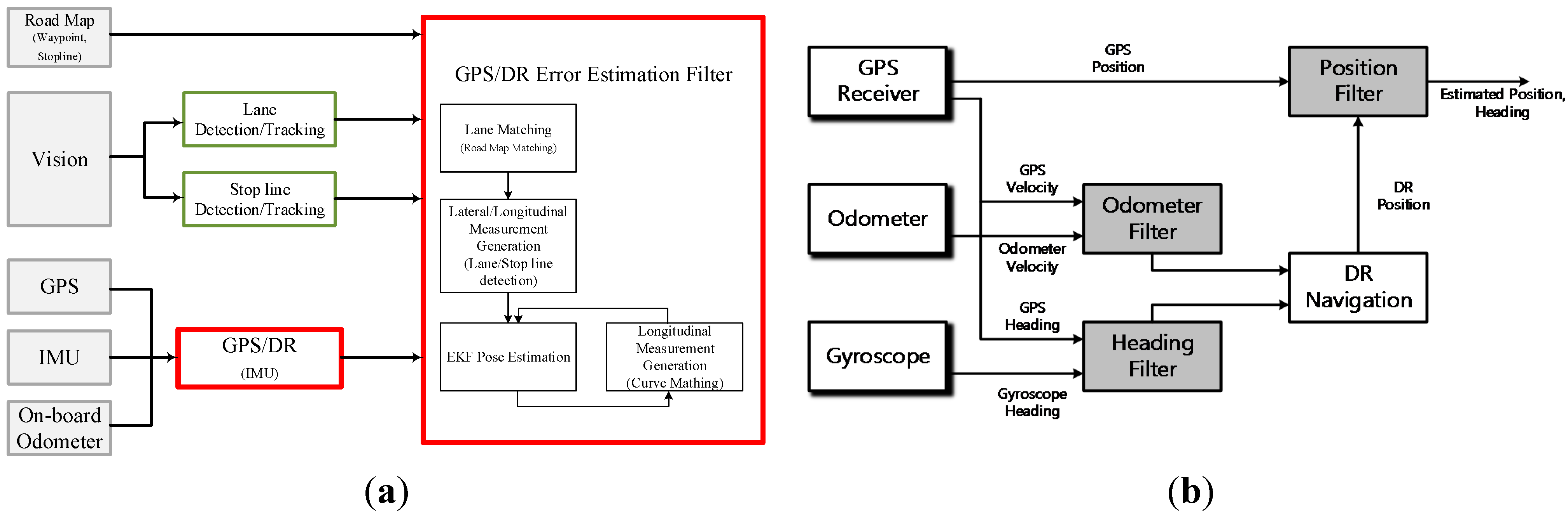
The proposed navigation system consists of a GPS, an Inertial Measurement Unit (IMU), an odometer, a map and a vision sensor (
Figure 1a). The GPS/DR system consists of a GPS receiver, an odometer and a gyroscope (
Figure 1b), and it provides the position and heading angle. The odometer filter estimates the velocity of the vehicle, the heading filter estimates the heading angle, and the position filter estimates the position and the heading of the GPS/DR system. The GPS/DR system model is summarized as follows.
Figure 1.
(a) Overall system structure; (b) GPS/DR system structure.
Figure 1.
(a) Overall system structure; (b) GPS/DR system structure.
In this equation, is the scale factor error of odometer, measurement is the difference between GPS and odometer speed and n is number of odometer pulses.
In this equation, and represent the heading angle error of the vehicle and the bias error of the gyroscope, is the measurement when the vehicle moves, and is the measurement when the vehicle stopped.
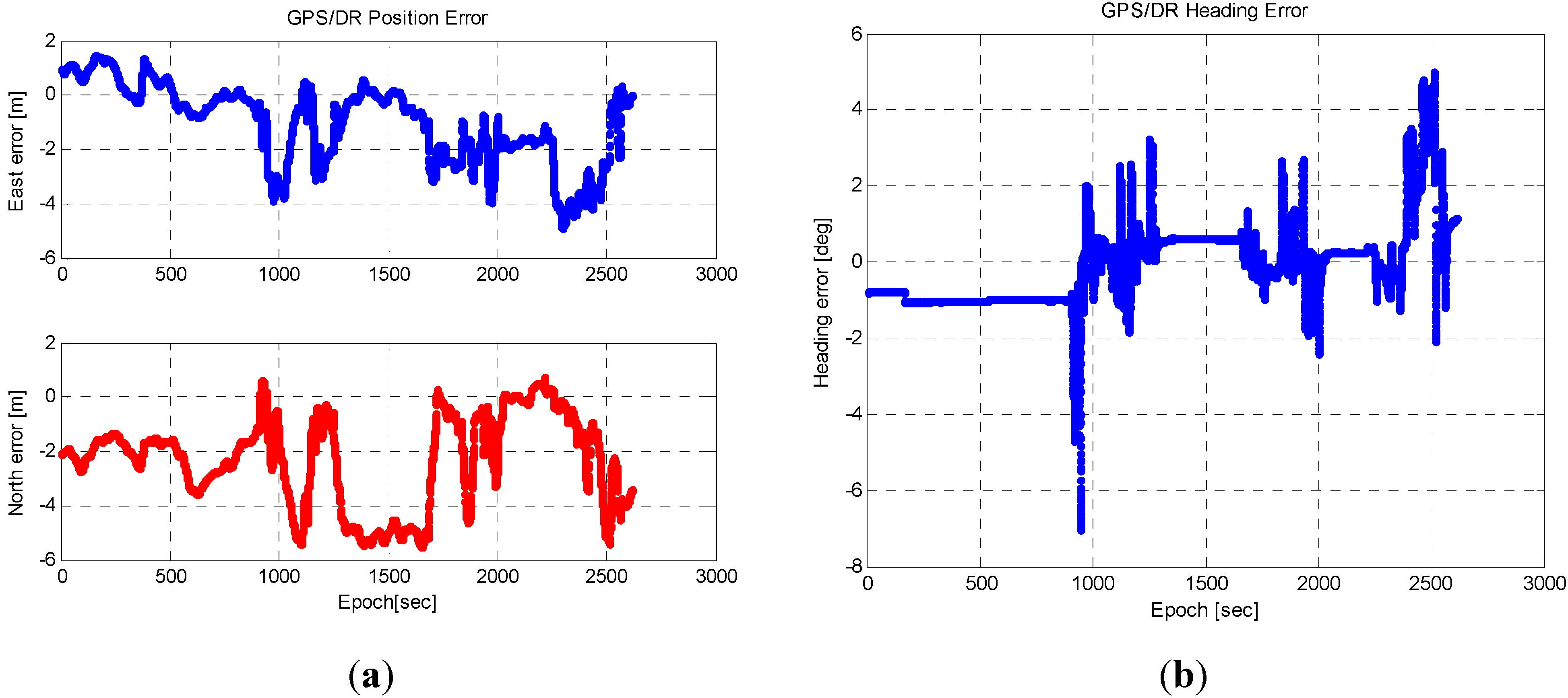
Figure 2 shows the performance of the estimated position/velocity of the GPS/DR system.
Image processing is used with a vision sensor to detect and track lanes and stop lines, and this information is used to measure the lateral and longitudinal distances.
An EKF-based GPS/DR error estimation filter estimates the GPS/DR error using lateral/longitudinal distance measurements that are obtained from the image processing system. In this study, we have assumed that the waypoint (map) is very accurate, and it makes GPS/DR error estimation possible. If the waypoint has an error, then the error is considered as a GPS/DR position error. Thus the positioning result of the proposed system is not sufficiently accurate in a global frame (erroneous latitude and longitude) but is accurate in a waypoint frame to make safe autonomous driving possible.
Figure 2.
(a) GPS/DR position error; (b) GPS/DR heading error.
Figure 2.
(a) GPS/DR position error; (b) GPS/DR heading error.
4.1. GPS/DR Error Modeling
In an open sky, the error components can be modeled by using the Dilution of Precision (DOP) error component that results of the placement of the satellites with the exception of the thermal noise, clock errors and the atmosphere error components [
19,
20]. The range measurements that can be obtained from a satellite can be modeled as follows:
In this equation,
is the range measurement of a satellite
,
,
,
,
,
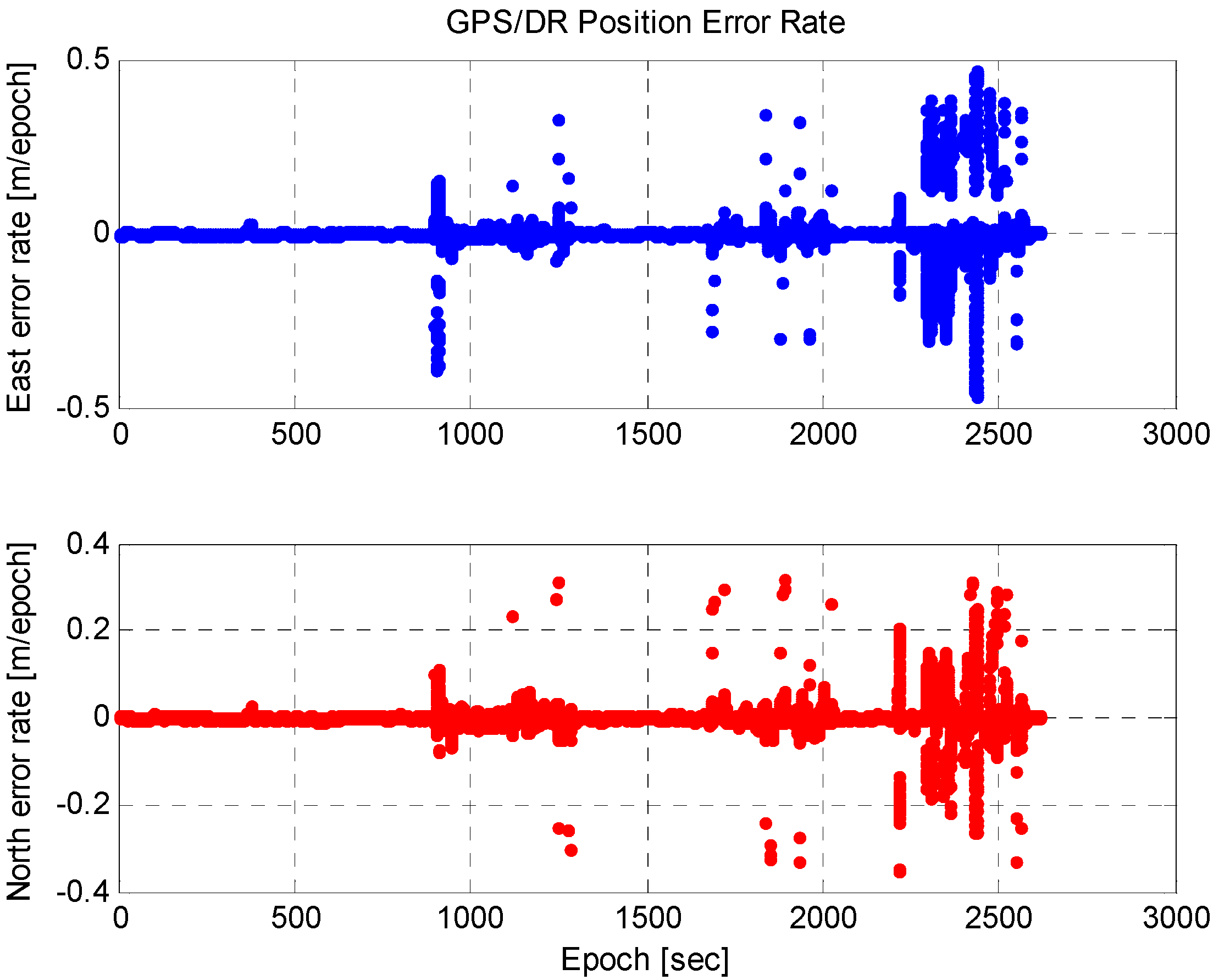
, represent the geometrical distance between a satellite and a receiver, the orbit error of a satellite, the clock error of a satellite, the clock error of the receiver, the atmospheric error (the delay error due to the ionosphere and troposphere), and the thermal noise of the receiver, respectively. At least four range measurements are required to calculate the position, and non-lane areas are very short during autonomous driving. At an intersection, the length of the section is shorter than 100 m and can be driven within 10 s at a speed of 36 km/h. We can assume that there is no change in the DOP during short intervals, and therefore, GPS errors can be modeled as a random constant. As shown in
Figure 3, the random constant model is appropriate because the change in the GPS/DR position error is small. We correct the GPS/DR position with the estimated GPS error by using the waypoint and vision in the lane or by predicting the GPS/DR error in the non-lane [
21]:
shows the east and north GPS/DR errors as state variables.
Figure 3.
GPS/DR position error rate.
Figure 3.
GPS/DR position error rate.
4.2. Curve Model Lane Detection, Curved Parameter Estimation and Lateral Measurement
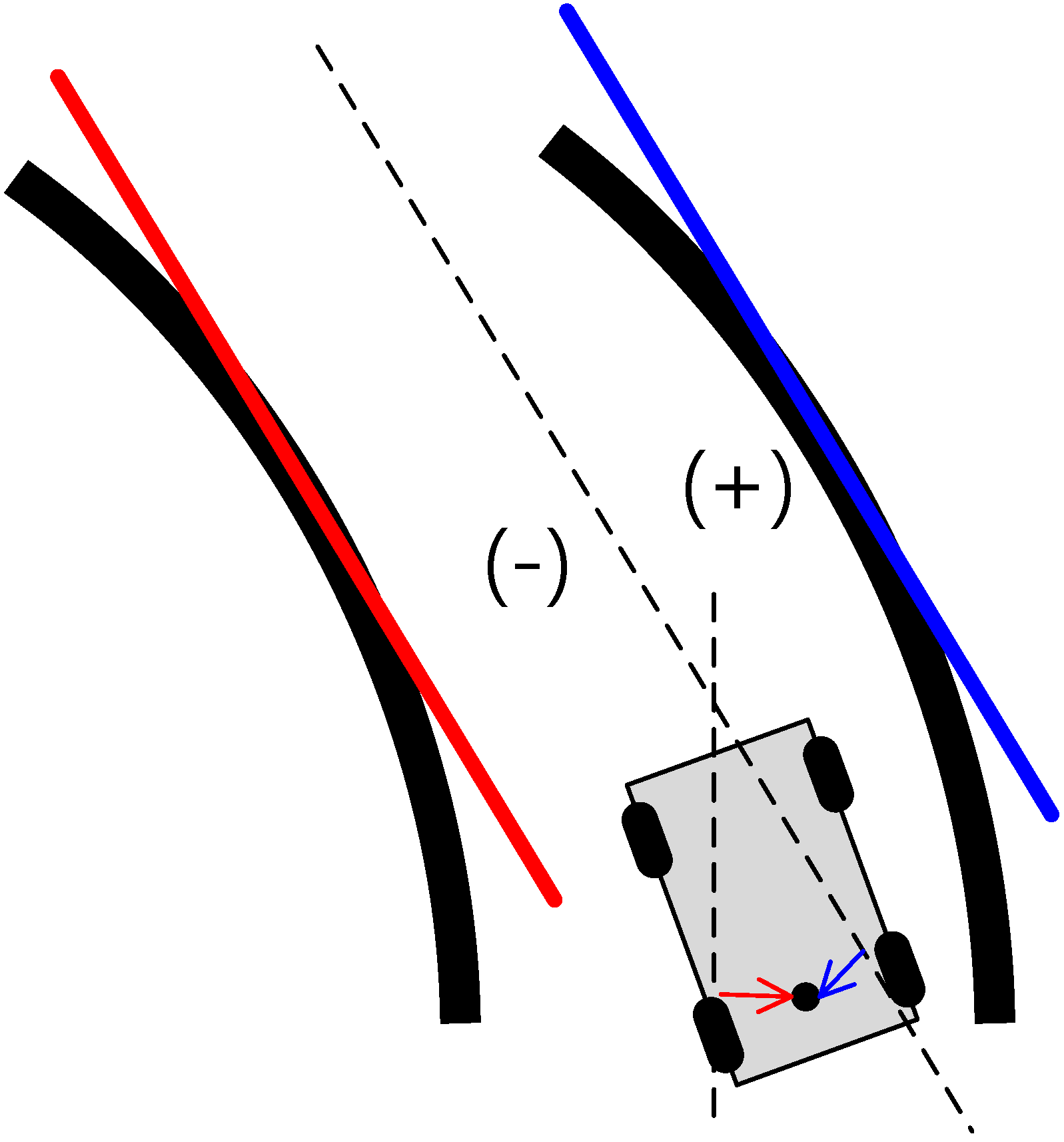
In general, the lane detection methods trace the vanishing points by using a straight line model [
22]. When the lane detection methods use a straight line model, an error can occur when lateral measurements are made in sections with a curved line (
Figure 4).
Figure 4 shows that the origin of the vehicle is on the right side of the lane (+), but errors occur in the estimation of the left side of the lane (−) during lane detection using straight line models. Therefore, lane detection is carried out using curved models to remedy these errors.
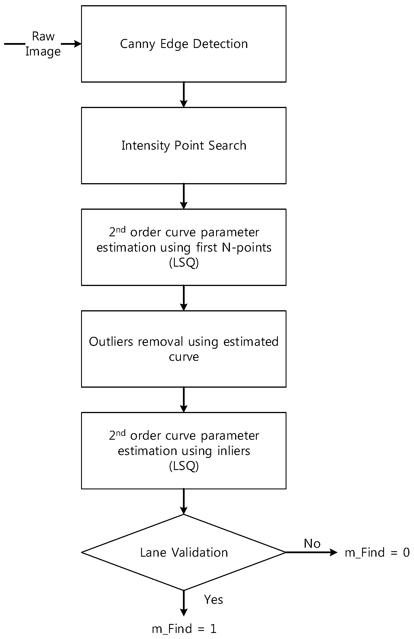
Figure 5 consists of a flow chart of the lane detection with curved models. The curved parameters of the lane are estimated by generating a model with a second-order polynomial line by using the least squares (LSQ) method with a simple edge detector, finding pixels that are considered to indicate lanes, and using
n points among them. Subsequently, an outlier is removed by using the estimated line for the curve, as in
Figure 6.
Figure 4.
Lateral error during lane detection with a straight line model.
Figure 4.
Lateral error during lane detection with a straight line model.
Figure 5.
Flowchart for the lane detection in a curved model.
Figure 5.
Flowchart for the lane detection in a curved model.
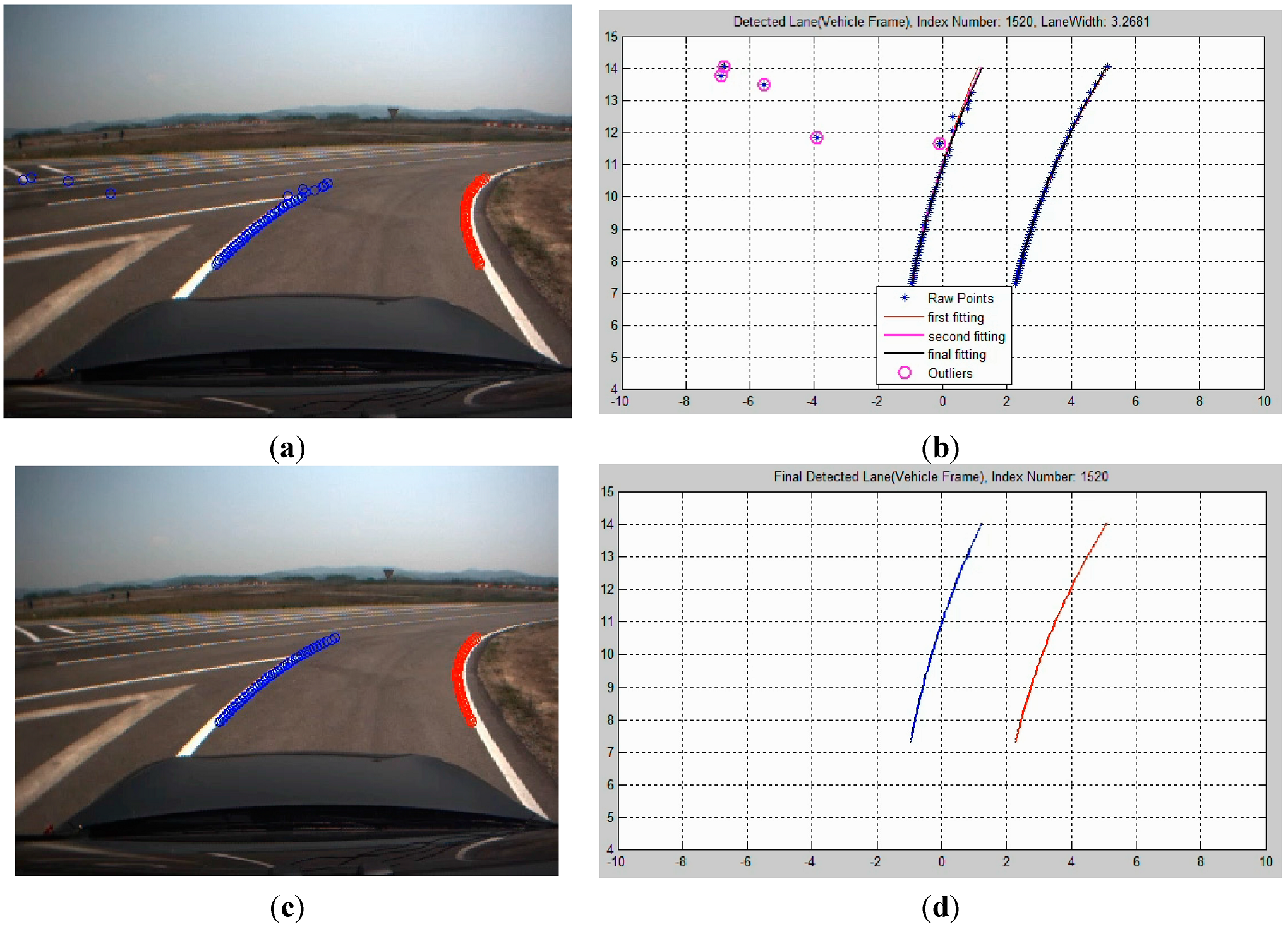
Figure 6.
Removal of the outliers through curved model estimation: (a) image frame; (b) vehicle frame; (c) before the outlier removal; (d) after the outlier removal.
Figure 6.
Removal of the outliers through curved model estimation: (a) image frame; (b) vehicle frame; (c) before the outlier removal; (d) after the outlier removal.
The constraints of the lane validation method used in this paper are as follows:
- (1)
The width of both lanes that are detected is 2.5–4.5 m. The width of the general lane is about 3.5 m.
- (2)
The difference in the slopes (the first-order term) for both lanes is less than 0.3 because the lanes are parallel.
- (3)
The difference in the angle variation (the second-order term) for both lanes is below 0.015 because the variation in the angle of both lanes is the same as that in curved sections.
The length of the area is confined to be 14 m in order to minimize the distortion that occurs during transformation from an image frame to a vehicle frame, and , are also set.
To obtain stable lateral measurements, the curved parameter (
) is estimated by using a Kalman filter with the points predicted for the outlier-removed lanes and the curved models consist of the second-order polynomial models from Equation (6):
This simple model is used with vehicles that move at a speed of
ν, as measured by the odometer of the vehicle, and the filter equation is as follow with
[
23,
24].
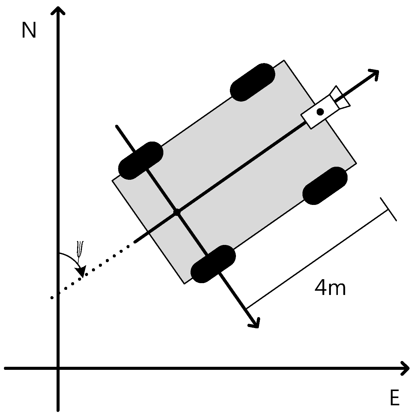
The frame is the vehicle frame (
Figure 7) with
detected lane points in the vehicle frame. The points detected on the Y axis for both lanes is estimated using a LSQ method that corresponds to
.
Figure 7.
Global frame and vehicle frame.
Figure 7.
Global frame and vehicle frame.
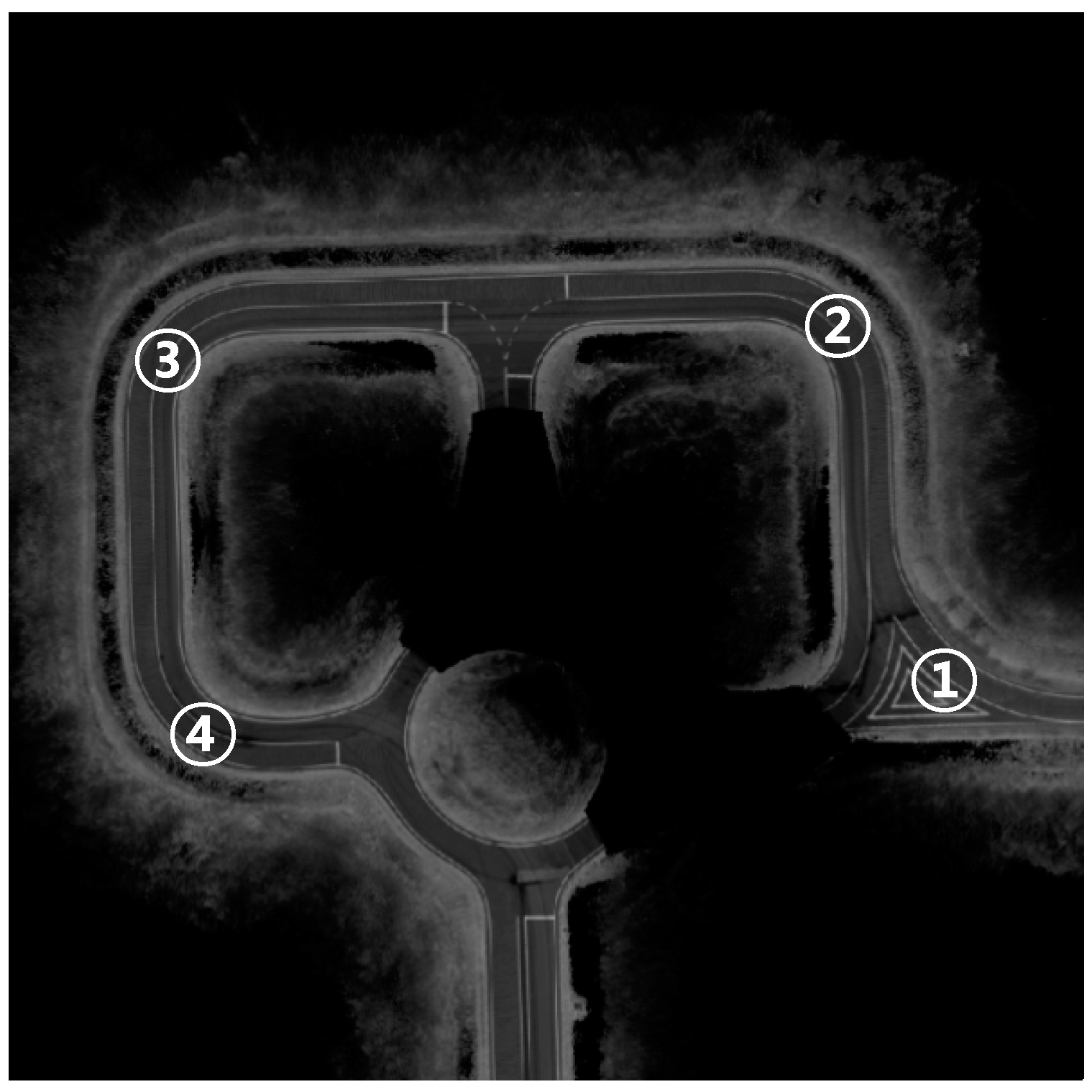
Figure 8 represents the lateral measurements for all sections and the section that is indicated has a sharp curved lane that appears sequentially (
Figure 9).
Figure 8.
Lateral measurements for lane detection: (a) in a straight line model; (b) in the curved model.
Figure 8.
Lateral measurements for lane detection: (a) in a straight line model; (b) in the curved model.
Figure 9.
Curved lane sections.
Figure 9.
Curved lane sections.
The results were obtained using driving data that was obtained from the center of the lanes with manual driving. Therefore, the lateral measurements should have a value near zero. In
Figure 9, area ① is a right turn, and ②–④ are a left turn. As shown in
Figure 8a, the errors indicate that the vehicles are located in the left of the lane in the left turn area and that vehicles are located on the right side of the lane in the right turn area. As the curved lane sections become sharper, the errors increase. If this measurement is used, the GPS/DR errors can be incorrectly estimated. However,
Figure 8b shows lateral measurements close to zero with the second-order polynomial models. In other words, the estimation functions for GPS/DR errors can be improved by using curved models.
4.3. Longitudinal Measurements from the Stop Line Detection
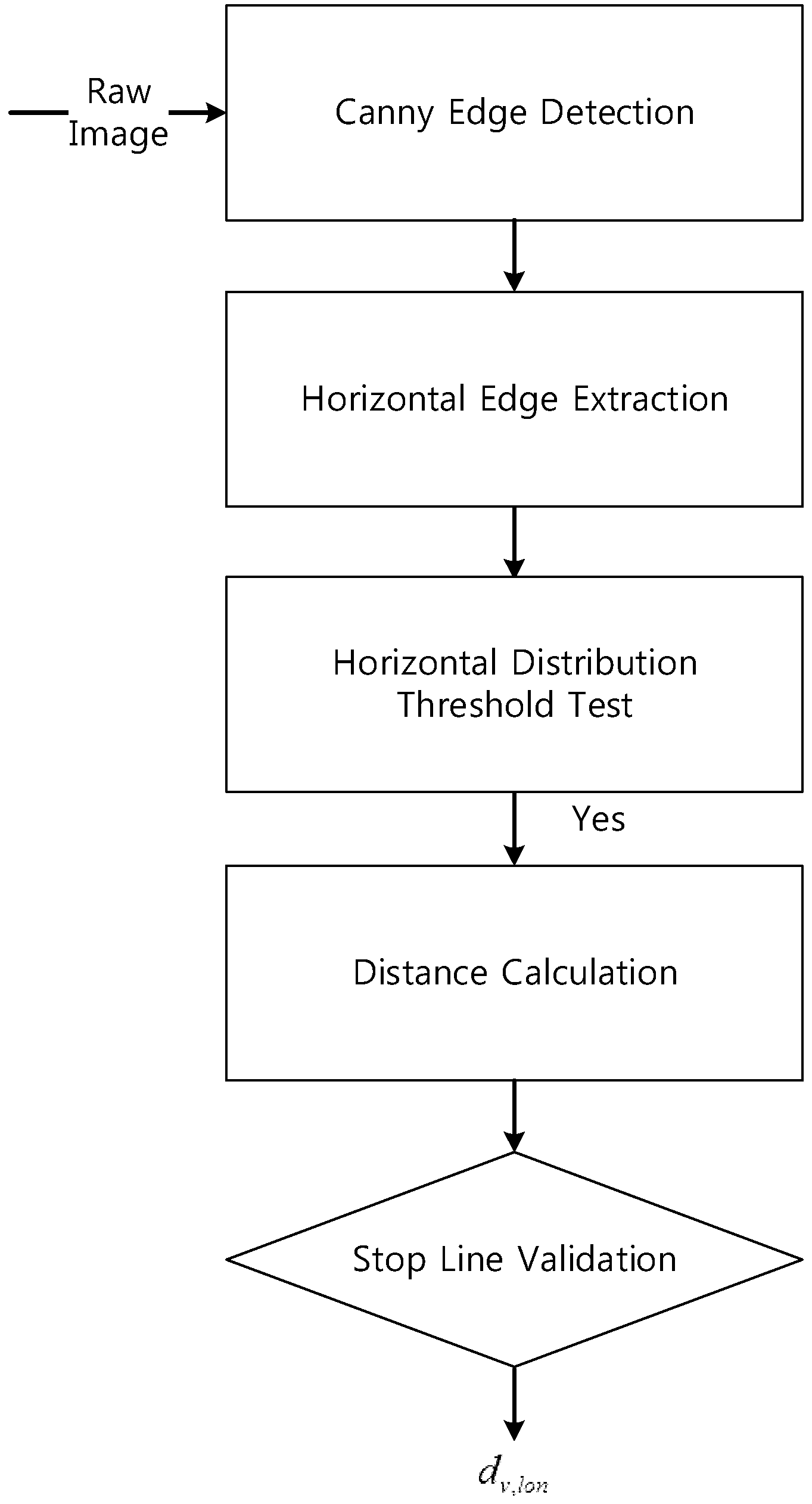
An accurate position in terms of the lateral lanes is used to keep the vehicle in the center of the lane. However, the accuracy of the longitudinal position is important in order to enact changes in the direction when in an intersection. Stop lines can be detected using vision sensors, and the stop lines that are detected are thus used to calculate the longitudinal measurements.
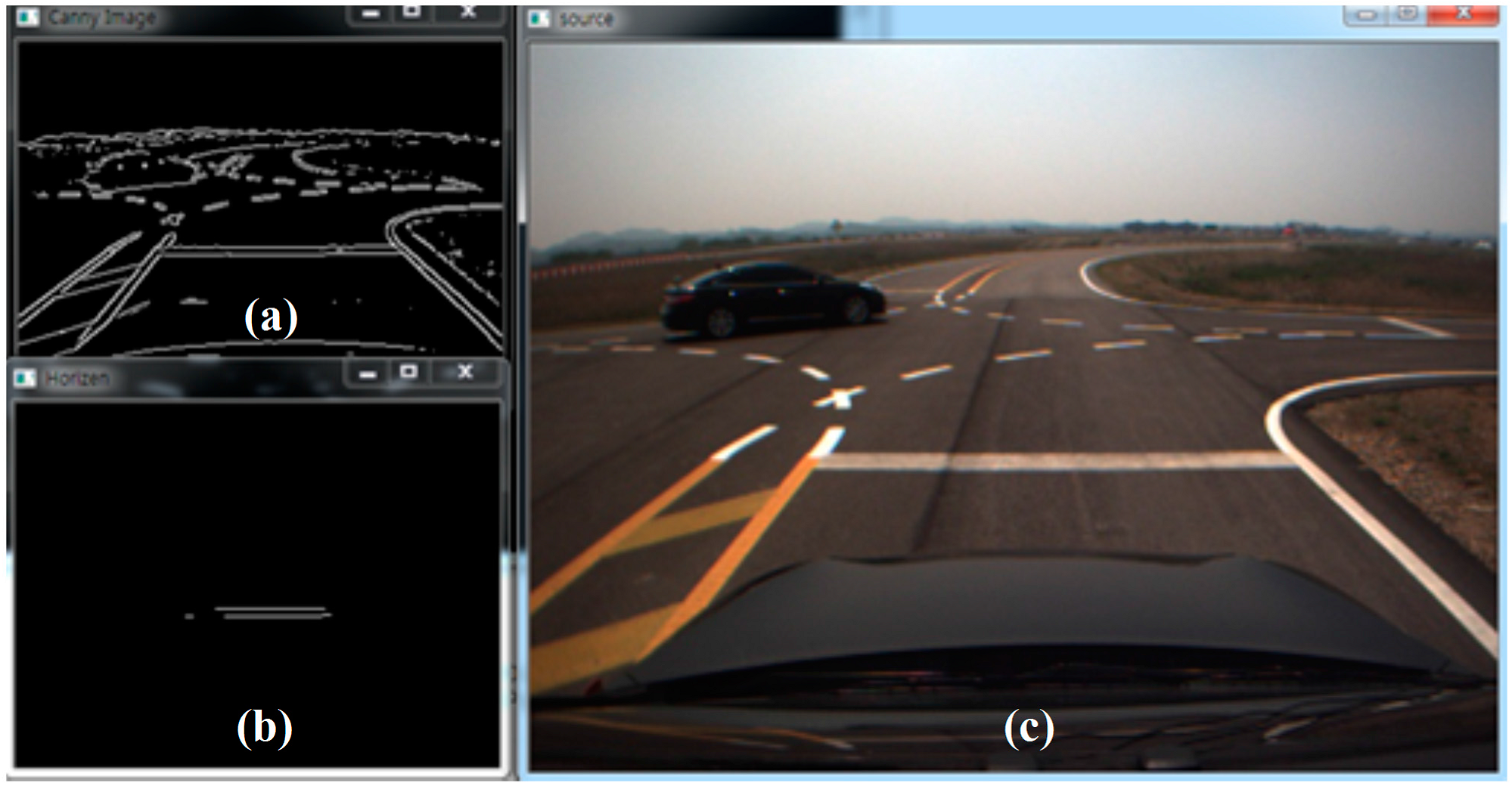
Figure 10 shows the flowchart of stop line detection and the result is shown as
Figure 11. The constraints of the validation of the distance for the detected stop lines are as follows:
- (1)
The stop line is located laterally within 3.5 m.
- (2)
The stop line measurement is less than 14 m (which is the reliable range of vision calibration in this test).
- (3)
The difference between the detected stop line location and the map is less than 3 m (feasible GPS/DR error).
Figure 10.
Flowchart for the stop line detection.
Figure 10.
Flowchart for the stop line detection.
Figure 11.
Result of the stop line detection: (a) Canny edge detection; (b) detected stop line; (c) raw image.
Figure 11.
Result of the stop line detection: (a) Canny edge detection; (b) detected stop line; (c) raw image.
4.4. GPS/DR Error Estimation Filter
The error estimation filter uses measurements from both sensors, including GPS/DR and a vision sensor. GPS/DR provides information on the absolute position, and the vision sensor provides information on the vehicle frame that is different from that of GPS/DR. Therefore, the error estimation filter has a structure where the information of the navigation frame is corrected by using information that is measured for the vehicle frame [
25]. The lateral distance between the GPS/DR and the waypoint link can be calculated by using a waypoint as the information of a map. For the vision sensor, the lateral distance from the center of the lane can be measured by detecting the lanes. This study makes two assumptions for the error estimation filter:
Assumption 1:
The waypoint is located at the center of the lanes. In general, the location information for the lanes is produced through a survey when accurate maps are produced, and therefore, the center of the lanes can be easily extracted from an accurate map that has been produced.
Assumption 2:
The waypoints in the curved section are very fine, so the vehicles do not go outside of the lane.
The measurement that was used for the error estimation filter utilizes the lateral distance from the center of lanes that was measured with the vision sensor (
), and the lateral distance is calculated by using the GPS/DR and the waypoint (
). The longitudinal distance uses
and
, which are obtained from the vision sensor and from GPS/DR, respectively. Therefore, the measurement equation is shown in Equation (14):
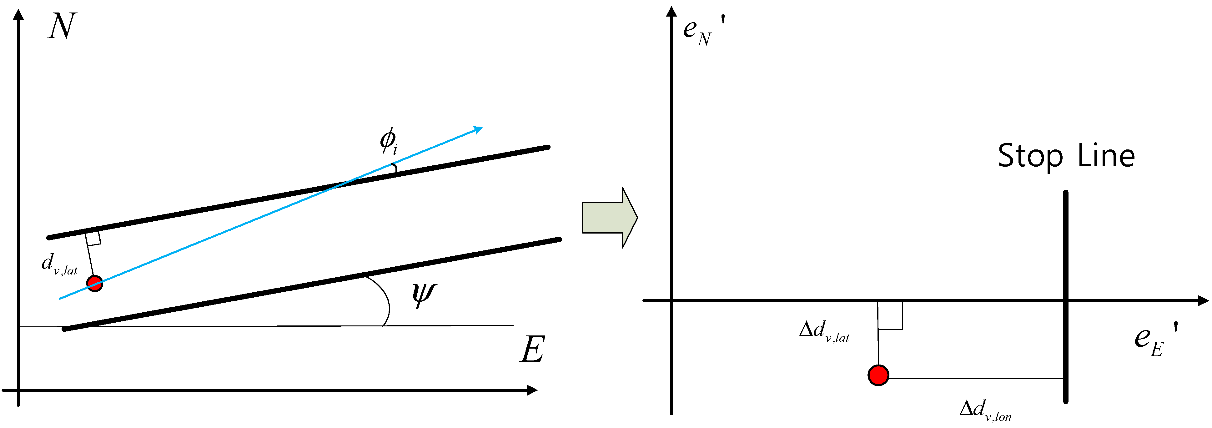
It is necessary to present the lane frame to configure the filter (
Figure 12), and as shown in
Figure 12, the frame is rotated according to the heading angle (
) and is calculated from a waypoint. Then, it can be transformed into a lane frame:
After the rotation, the transformed
axis corresponds to a lane. This is the lateral distance information of the lanes, and therefore, the equation for the lane frame can be presented as follows:
Equation (19) can be obtained through a partial differential of each term in Equation (18):
The GPS/DR error estimation filter can be summarized as follows:
State equation:
Measurement equation:
4.5. Longitudinal Measurement from the Curve Matching
The longitudinal position error from the GPS/DR measurement may be large in the transition area from a straight to a curved lane when the vehicle starts to drive or drives in one direction for a long time because there is no longitudinal information. If the vehicle enters a curved section, the heading of the vehicle and the waypoint change, and then the error estimation for east and north become available. However, before entering a curve, the waypoint navigation may suffer from a failure due to the steering command that has been generated with an incorrect timing as a result of the longitudinal error.
The curved parameter of the lane ahead can be calculated as in Equation (6) by using the waypoint. After interpolation with a resolution of
, the waypoint that uses the curved parameter that has been calculated is transformed into a vehicle frame. At this time, the transformation uses the corrected position with the error estimator that has been laterally corrected. Then the interpolated waypoint curve (
) has no lateral distance with the curve (
) that is detected from the image and only has a longitudinal distance because the lateral error of the GPS/DR has already been estimated. The error function that measures the longitudinal range is shown in Equations (27) and (28):
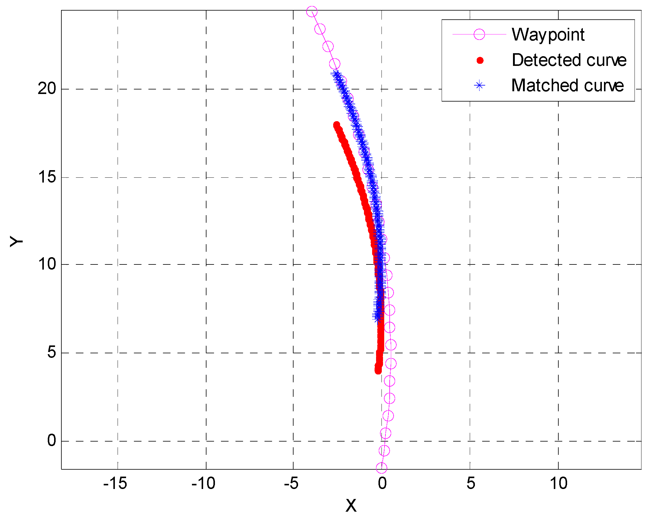
As shown in
Figure 13, the true longitudinal distance is −2.78 m, and the distance measured (
) from Equation (28) is −2.93 m. Thus, accurate longitudinal measurements can be obtained through curve matching.
The measurements for the longitudinal range from the curve matching are effective only in the transition from a straight to a curved lane. After the longitudinal error has been estimated once, the lateral information in the area of the curve becomes longitudinal information. Therefore, in this study, we have used
and have restricted the section where curve matching was performed by the waypoint curvature. The longitudinal range that was measured is used as an input of the error estimation filter that is described in
Section 4.4.
Figure 13.
Measuring the longitudinal distance with curve matching (: waypoint curve; : detected curve lane, : matched curve).
Figure 13.
Measuring the longitudinal distance with curve matching (: waypoint curve; : detected curve lane, : matched curve).
5. Autonomous Experimental Results
The experiment was carried out by applying the lane detection method with a curved model and the GPS/DR error estimation filter proposed in this study in an autonomous vehicle.
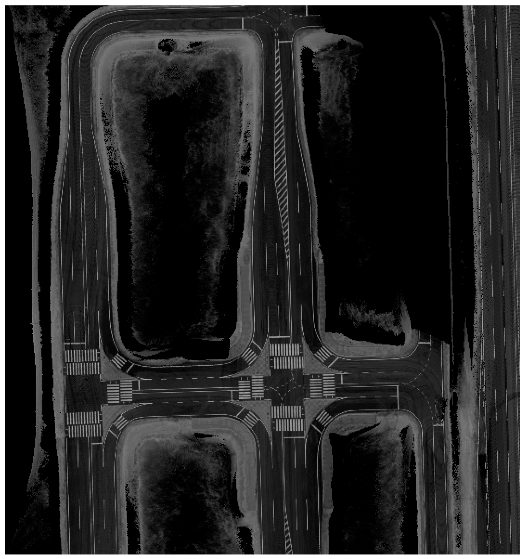
Figure 14 shows a map that is based on the reflectivity of the experimental site. The map was produced by using a commercial RTK/INS system and a 3D-LiDAR (HDL-32E, Velodyne, Morgan Hill, CA, USA) (
Table 1).
Figure 14.
Reflectivity map.
Figure 14.
Reflectivity map.
Table 1.
Experimental environment.
Table 1.
Experimental environment.
| GPS/DR | Vision Sensor | Reference Trajectory |
|---|
| U-Blox EVK 6T + ADIS 16405 | BumbleBee 2 | Commercial RTK/INS (Novatel Propak V3 + SPAN HG1700) |
The true value of the position cannot be known due to the movement in the environment, so a commercial RTK/INS system, which has a high price, was used to determine the reference position (true value) to conduct a quantitative analysis.
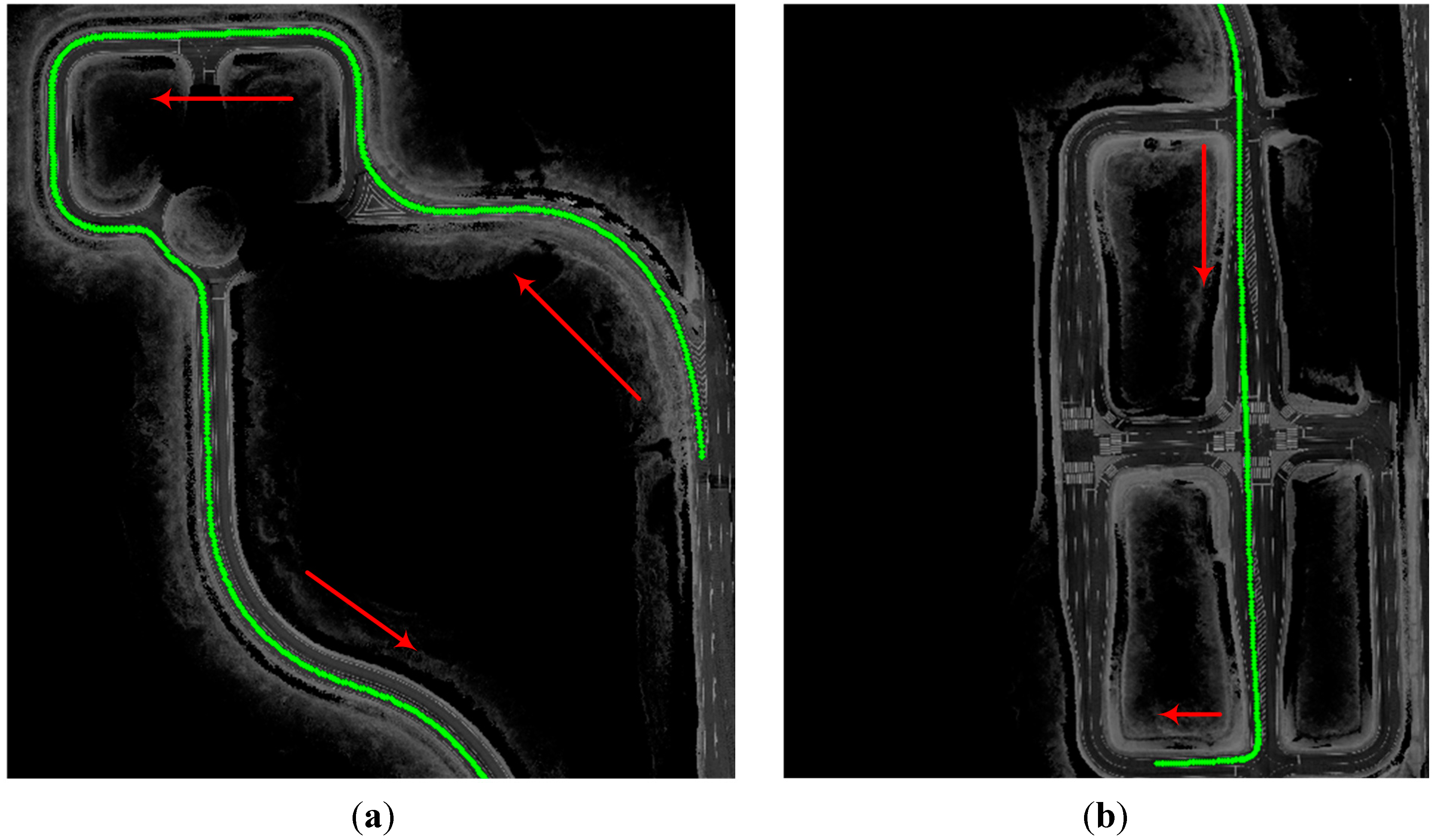
Figure 15 shows the total trajectory.
Figure 15.
Driving trajectory (arrows represent the direction of vehicle). (a) curved section; (b) intersection.
Figure 15.
Driving trajectory (arrows represent the direction of vehicle). (a) curved section; (b) intersection.
Figure 16 shows the results that were obtained with the proposed method, and
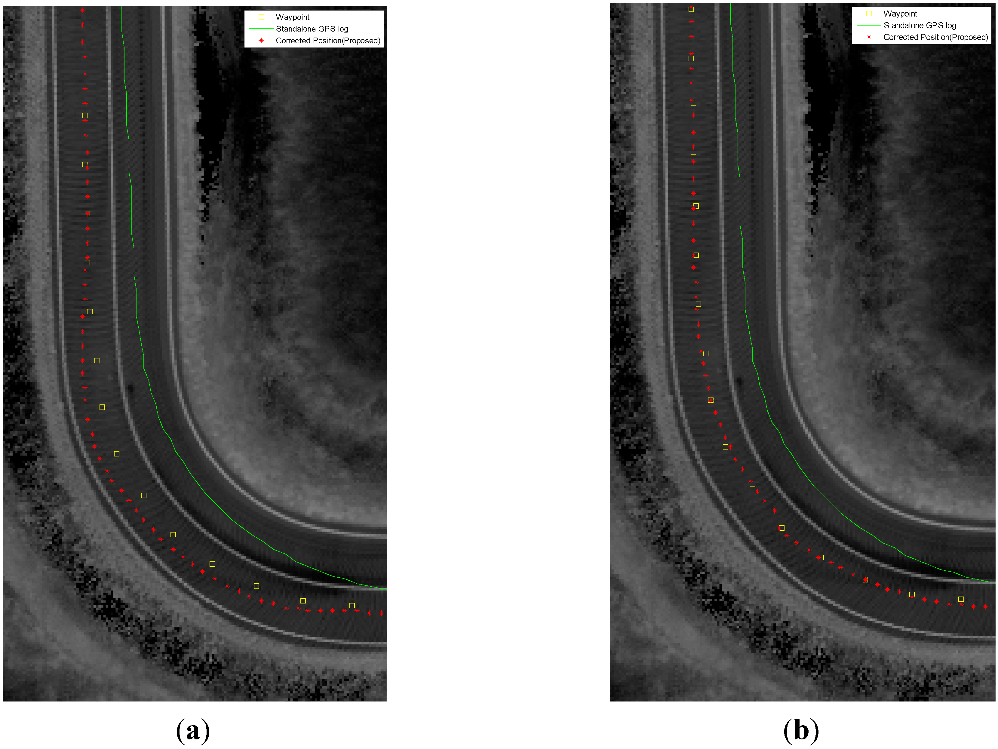
Figure 17 shows a comparison of the results when measurements were used for lane detection with a straight line model and with a curved model in sections with sharp curves. In this section, the result of using a straight model is that vehicles lean to the left during a right turn and to the right during a left turn. However, the results when using a curved model reduce the lateral error.
Figure 16.
Estimated GPS/DR lateral error (red) and position error (blue).
Figure 16.
Estimated GPS/DR lateral error (red) and position error (blue).
Figure 17.
Experimental results for the curved lane sections: (a) straight model; (b) curved model (□: waypoint, -: Standalone GPS/DR, *: proposed).
Figure 17.
Experimental results for the curved lane sections: (a) straight model; (b) curved model (□: waypoint, -: Standalone GPS/DR, *: proposed).
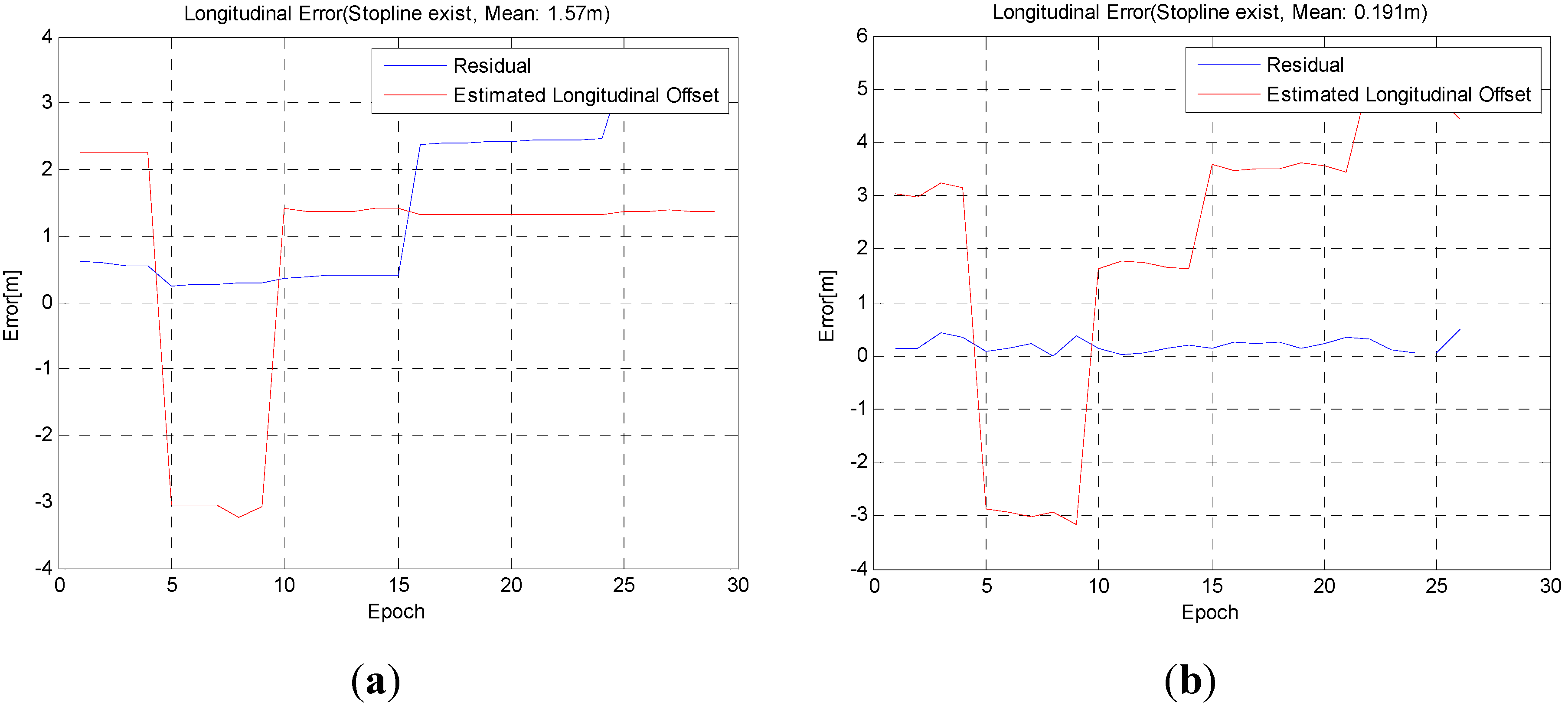
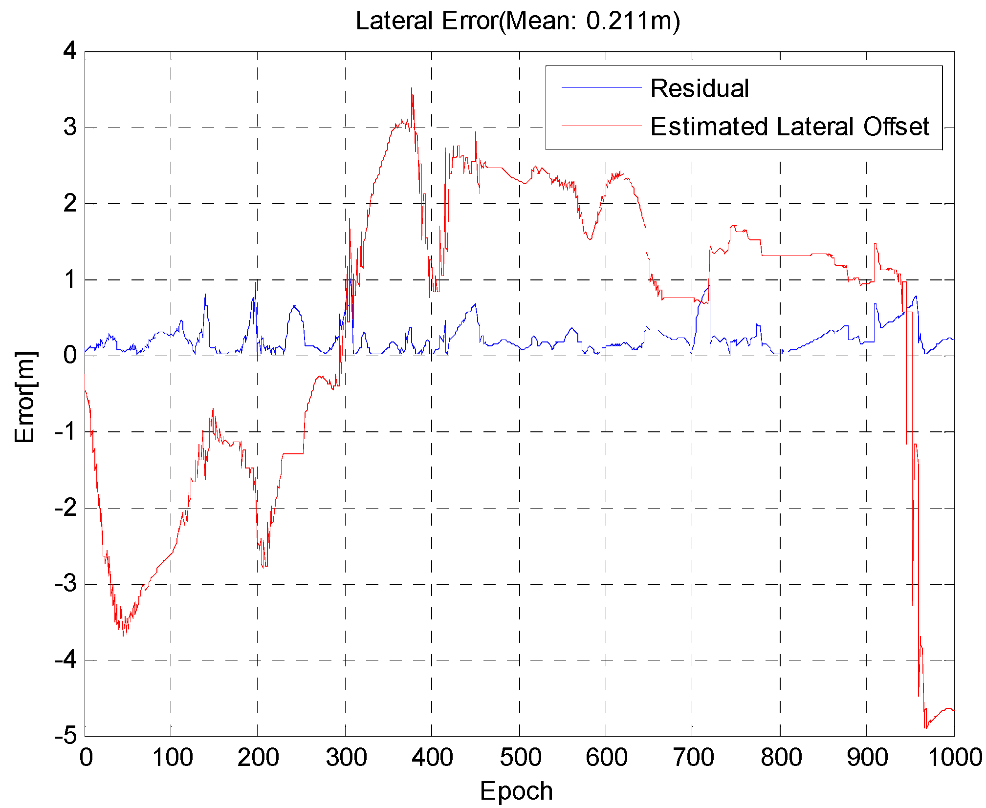
A stop line does not exist in every section, and therefore, the longitudinal accuracy analyzes the sections with stop lines (
Figure 18).
Figure 18.
Estimated GPS/DR longitudinal error (red) and position error (blue): (a) without stop line detection; (b) with stop line detection.
Figure 18.
Estimated GPS/DR longitudinal error (red) and position error (blue): (a) without stop line detection; (b) with stop line detection.
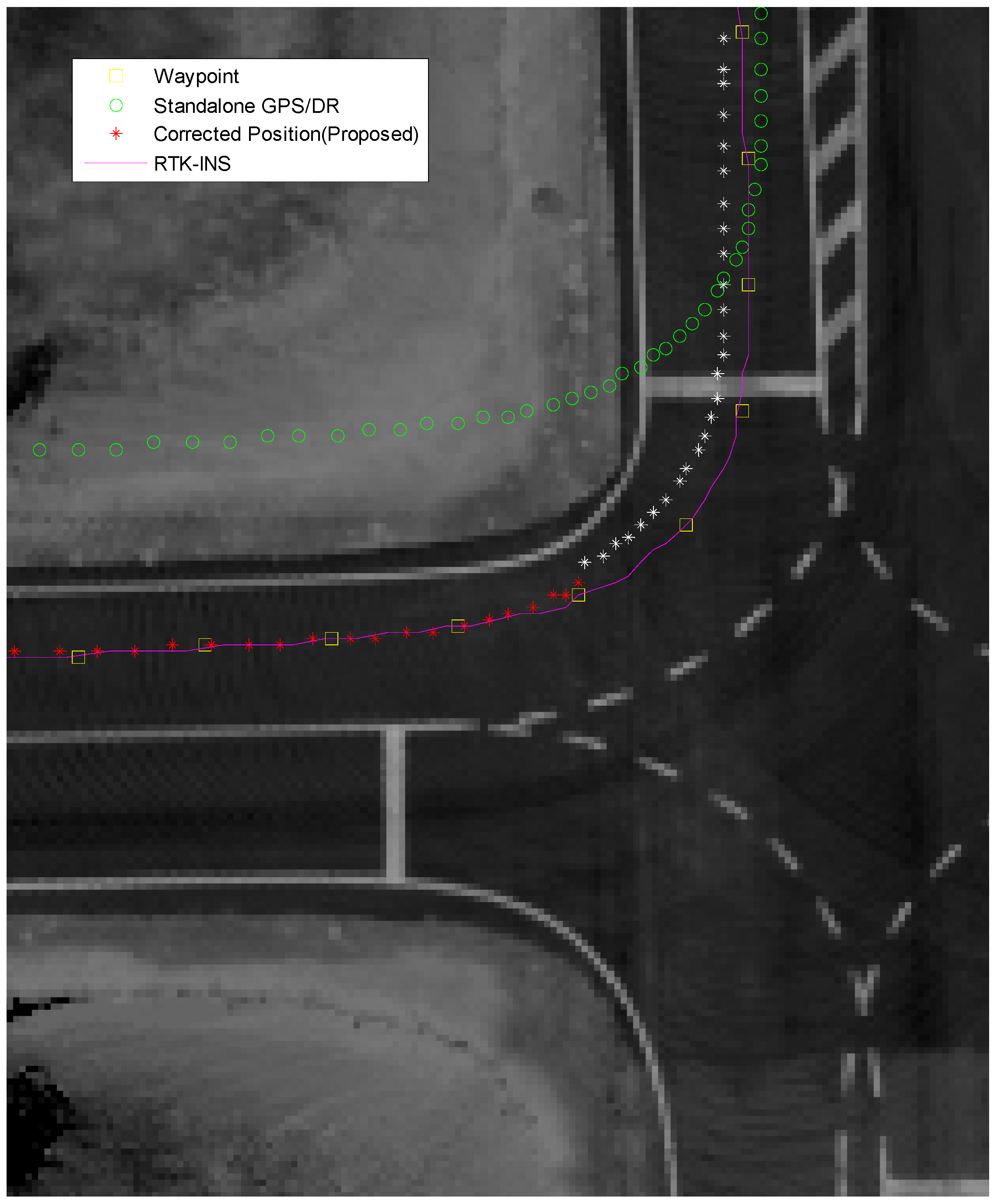
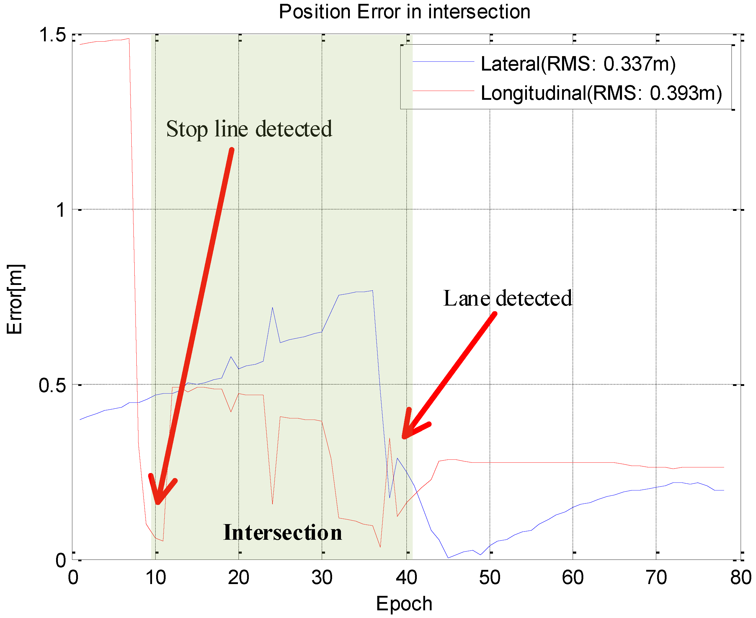
Figure 19 and
Figure 20 show the results in an intersection and the white asterisk indicates the results where no vision measurements have been taken. Even in this section, vision information cannot be obtained, we derived the position with a sub-meter level of accuracy.
Figure 19.
Result at the intersection (□: waypoint, o: GPS/DR, *: proposed, -: RTK/INS).
Figure 19.
Result at the intersection (□: waypoint, o: GPS/DR, *: proposed, -: RTK/INS).
Figure 20.
Position error at the intersection.
Figure 20.
Position error at the intersection.
In
Table 2, the overall longitudinal error is larger than the intersection. The reason for this is that the longitudinal error can be corrected before entering an intersection, but cannot be estimated because most of total trajectory is straight.
Table 2.
Result summary.
| RMSE (m) | GPS/DR | Overall | w/o Stop Line | With Stop Line | Intersection |
|---|
| Lateral | 1.77 | 0.217 | - | - | 0.337 |
| Longitudinal | 2.11 | 0.618 | 1.57 | 0.191 | 0.393 |
6. Conclusions
This study proposes a navigation system that supports autonomous driving through the use of GPS/DR, waypoints and a vision sensor. The disadvantages of using a lane following system with lane detection is that there are discontinuous sections in the lanes. Therefore, this study proposed a GPS/DR error estimation filter that allows stable navigation in such sections. In addition, we suggest methods that can reduce the errors in the lateral distance by detecting lanes using a curved model in order to solve the problems where lateral distance errors occur in curved lane sections. The curve matching method between the waypoints and the detected curve lanes reduces the longitudinal error before entering a curved section after a straight section. Only lane and stopline detection was performed using image processing, so much less computational power is required when compared to the use of visual odometry and a particle filter, and it is thus very easy to enable real-time use in embedded systems.
This system can therefore be applied in not only an autonomous vehicle but also vehicles which is already equipped with GPS, IMU and black box(monocular vision sensor) to safely run the vehicle in straight lanes, curved lanes and through intersections.
However, greater availability is required for autonomous vehicles. The stopline was the only road marking considered in this paper for longitudinal information, but the stopline does not exist everywhere. Thus, every road marking (arrow, speed limit,
etc.) will be added to provide more longitudinal information. Also, vision sensors have limited functionality at night or with a backlight, so LiDAR, Dedicated Short Range Communications (DSRC),
etc. can possibly be used in autonomous vehicles [
26,
27,
28,
29]. Multi-sensor systems based on a federated Kalman filter can improve the reliability and availability of the localization system, and in addition, the integrity of an autonomous vehicle can be provided by using the covariance of local filters and the master filter. Therefore, a localization method that ensures the availability and integrity will be part of future work.
Acknowledgments
This research was supported by a grant from “Development of GNSS based Transportation Infrastructure Technology (06-A03)” funded by Ministry of Land, Infrastructure and Transport of Korean government.
Author Contributions
Designed the localization system and wrote the paper: B.H.L.; Contributed to discussion of result and provided significant suggestion: J.-H.S., J.-H.I., S.-H.I. and M.-B.H.; Supervised the research work: G.-I.J.
Conflicts of Interest
The authors declare no conflict of interest.
References
- Lee, B.H.; Jee, G.I. Performance analysis of GPS-RTK floating solution with Doppler measurement. In Proceedings of the IS-GPS/GNSS, Taipei, Taiwan, 26–28 October 2010; pp. 273–276.
- Serrano, L.; Kim, D.; Langley, R.B. A single GPS receiver as a real-time, accurate velocity and acceleration sensor. In Proceedings of the ION GNSS 17th ITM, Long Beach, CA, USA, 21–24 September 2004; pp. 2021–2034.
- Badino, H.; Huber, D.; Kanade, T. Visual topometric localization. In Proceedings of the IEEE Intelligent Vehicles Symposium, Baden-Baden, Germany, 5–9 June 2011; pp. 794–799.
- Du, J.; Barth, M.J. Next-Generation Automated Vehicle Location Systems: Positioning at the Lane Level. IEEE Trans. Intell. Transp. Syst. 2008, 9, 48–57. [Google Scholar]
- Laneurit, J.; Chapuis, R.; Chausse, F. Accurate vehicle positioning on a numerical map. Int. J. Control Autom. Syst. 2005, 3, 15–31. [Google Scholar]
- Miller, I.; Campbel, M.; Huttenlocher, D. Map-aided localization in sparse global positioning system environments using vision and particle filtering. J. Field Robot. 2011, 28, 619–643. [Google Scholar] [CrossRef]
- Dissanayake, M.W.M.G.; Newman, P.; Clark, S.; Durrant-Whyte, H.F.; Csorba, M. A solution to the simultaneous localization and map building (SLAM) problem. IEEE Trans. Robot. Autom. 2001, 17, 229–241. [Google Scholar] [CrossRef]
- Montemerlo, M.; Thrun, S.; Koller, D.; Wegbreit, B. FastSLAM: A factored solution to the simultaneous localization and mapping problem. In Proceedings of the AAAI National Conference on Artificial Intelligence, Edmonton, AB, Canada, 28 July–1 August 2002; pp. 593–598.
- Thrun, S.; Burgard, W.; Fox, D. Probabilistic Robotics; MIT Press: Cambridge, MA, USA, 2005. [Google Scholar]
- Levinson, J.; Montemerlo, M.; Thrun, S. Map-based precision vehicle localization in urban environments. In Proceedings of the Robotics: Science and Systems, Atlanta, GA, USA, 27–30 June 2007; pp. 121–128.
- Levinson, J.; Thrun, S. Robust vehicle localization in urban environment using Probabilistic Maps. In Proceedings of the IEEE International Conference on Robotics and Automation, Anchorage, AK, USA, 3–7 May 2010; pp. 4372–4378.
- Schreiber, M.; Knoppel, C.; Franke, U. LaneLoc: Lane marking based localization using highly accurate maps. In Proceedings of the IEEE Intelligent Vehicles Symposium, Gold Coast, Australia, 23–26 June 2013; pp. 449–454.
- Bak, A.; Gruyer, D.; Bouchafa, S.; Aubert, D. Multi-sensor localization—Visual odometry as a low cost proprioceptive sensor. In Proceedings of the 15th International IEEE Conference on Intelligent Transportation Systems, Anchorage, AK, USA, 16–19 September 2012; pp. 1365–1370.
- Cuong, N.V.; Heo, M.B.; Jee, G.I. 1-Point Ransac based robust visual odometry. J. Korean GNSS Soc. 2013, 2, 81–89. [Google Scholar]
- Scaramuzza, D.; Siegwart, R. Appearance-guided monocular omnidirectional visual odometry for outdoor ground vehicles. IEEE Trans. Robot. 2008, 24, 1015–1026. [Google Scholar] [CrossRef]
- Gruyer, D.; Belaroussi, R.; Revilloud, M. Map-Aided localization with lateral perception. In Proceedings of the IEEE Intelligent Vehicles Symposium, Dearborn, MI, USA, 8–11 June 2014; pp. 674–680.
- Ieng, S.S.; Gruyer, D. Merging lateral cameras information with proprioceptive sensors in vehicle location gives centimetric precision. In Proceedings of the 18th International Technical Conference on the Enhanced Safety of Vehicles (ESV), Nagoya, Japan, 19–22 May 2003.
- Li, H.; Nashashibi, F.; Toulminet, G. Localization for intelligent vehicle by fusing mono-camera, low-cost GPS and map data. In Proceedings of the International IEEE Annual Conference on Intelligent Transportation Systems, Madeira, Portugal, 19–22 September 2010; pp. 1657–1662.
- Bernhard, H.-W.; Herbert, L.; Elma, W. GNSS-Global Navigation Satellite Systems, GPS, GLONASS, Galileo & More; Springer-Verlag Wien: New York, NY, USA, 2008. [Google Scholar]
- Kaplan, E.D.; Hegarty, C.J. Understanding GPS: Principles and Applications; Artech House: Boston, MA, USA, 2005. [Google Scholar]
- Seo, S.H.; Lee, B.H.; Jee, G.I. Position error correction using waypoint and vision sensor. In Proceedings of the International Symposium on GNSS, Jeju, Korea, 18–20 October 2014; pp. 31–34.
- Kuk, J.G.; An, J.H.; Ki, H.Y.; Cho, N.I. Fast lane detection & tracking based on hough transform with reduced memory requirement. In Proceedings of the International IEEE Annual Conference on Intelligent Transportation Systems, Madeira, Portugal, 19–22 September 2010; pp. 1344–1349.
- Li, T.; Zhidong, D. A new 3D LIDAR-based lane markings recognition approach. In Proceedings of the IEEE International Conference on Robotics and Biomimetics, Shenzhen, China, 12–14 December 2013; pp. 2197–2202.
- Bevly, D.M. GNSS for Vehicle Control; Artech House Publishers: Boston, MA, USA, 2010. [Google Scholar]
- Lee, B.H.; Im, S.H.; Heo, M.B.; Jee, G.I. Error correction method with Precise Map Data for GPS/DR based on Vision/Vehicle Speed Sensor. In Proceedings of the ION GNSS+, Nashville, TN, USA, 16–20 September 2013; pp. 1260–1266.
- Alam, N.; Balaei, A.T.; Dempster, A.G. An instantaneous Lane-Level positioning using DRSC carrier frequency offset. IEEE Trans. Intell. Transp. Syst. 2012, 13, 1566–1575. [Google Scholar] [CrossRef]
- Chen, L.; Li, Q.; Li, M.; Zhang, L.; Mao, Q. Design of a multi-sensor cooperation travel environment perception system for autonomous vehicle. Sensors 2012, 12, 12386–12404. [Google Scholar] [CrossRef]
- Chu, T.; Guo, N.; Backen, S.; Akos, D. Monocular Camera/IMU/GNSS integration for ground vehicle navigation in challenging gnss environments. Sensors 2012, 12, 3162–3185. [Google Scholar] [CrossRef] [PubMed]
- Cong, L.; Li, E.; Qin, H.; Ling, K.V.; Xue, R. A performance improvement method for low-cost land vehicle GPS/MEMS-INS attitude determination. Sensors 2015, 15, 5722–5746. [Google Scholar] [CrossRef] [PubMed]
© 2015 by the authors; licensee MDPI, Basel, Switzerland. This article is an open access article distributed under the terms and conditions of the Creative Commons Attribution license (http://creativecommons.org/licenses/by/4.0/).


 ,
, 


