
Mass Load Distribution Dependence of Mass Sensitivity of Magnetoelastic Sensors under Different Resonance Modes

Abstract
:1. Introduction
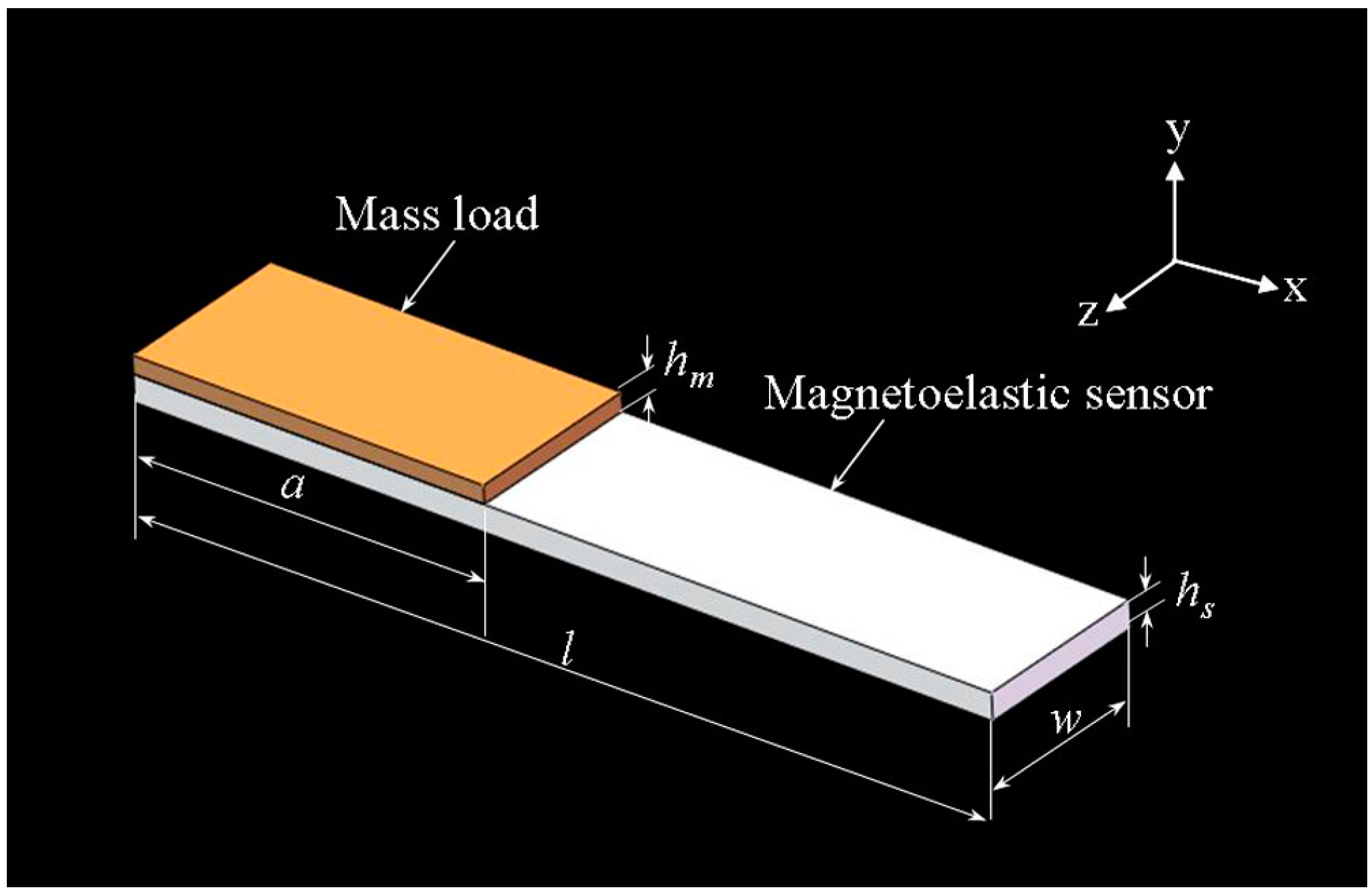
2. Theory


| Symbol | Unit | Value | |
|---|---|---|---|
| Young’s modulus | E | GPa | 105 |
| Density | ρs | kg/m3 | 7.9 × 10³ |
| Poisson’s ratio | ν | - | 0.33 |
| Length | l | mm | 1 |
| Width | w | mm | 0.2 |
| Thickness | hs | μm | 15 |
| a/l | - | - | 0.1, …, 1.0 |
| Mass ratio per unit length | ρmAm/ρsAs | - | 10−3 |
3. Results and Discussion
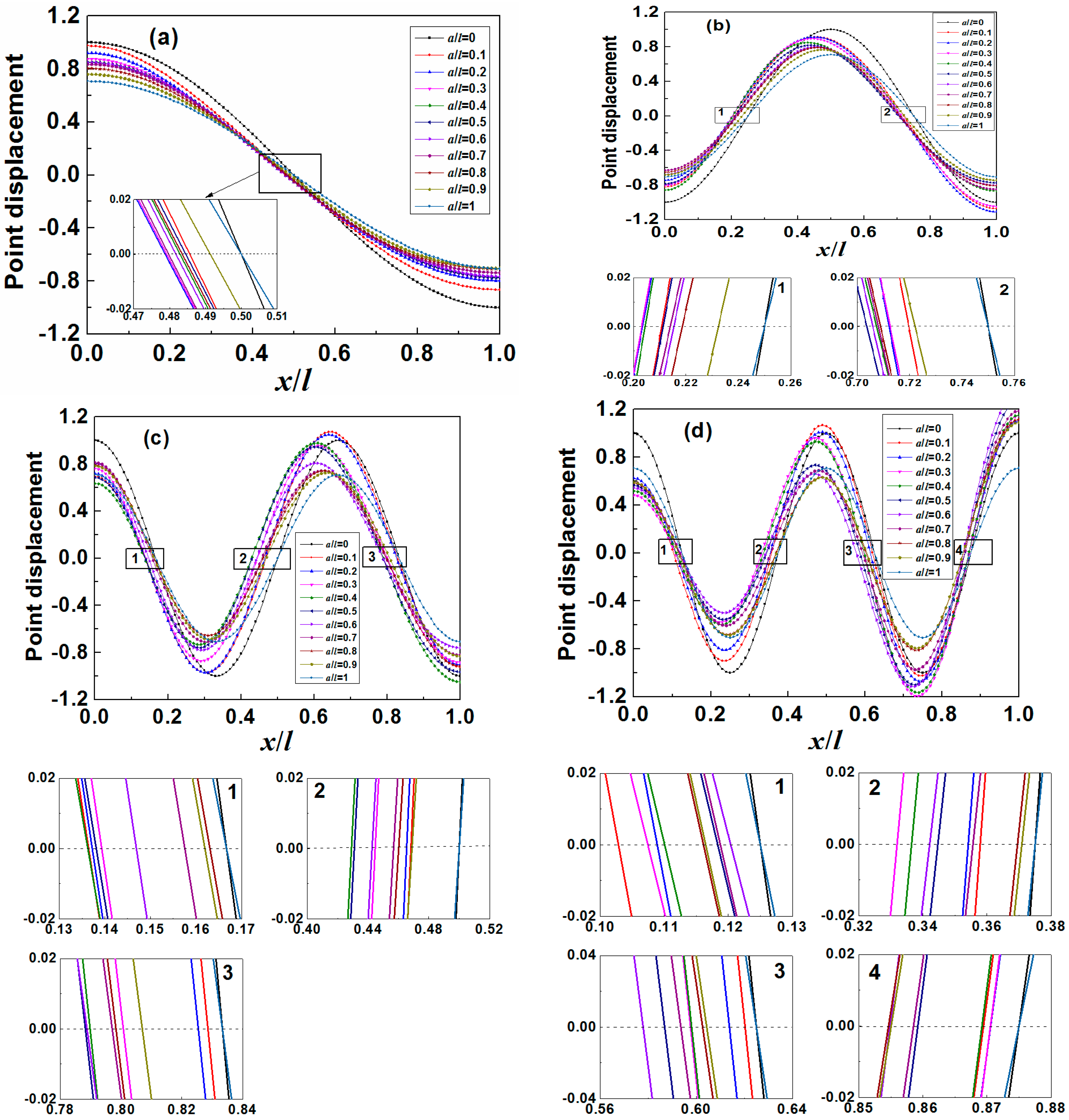
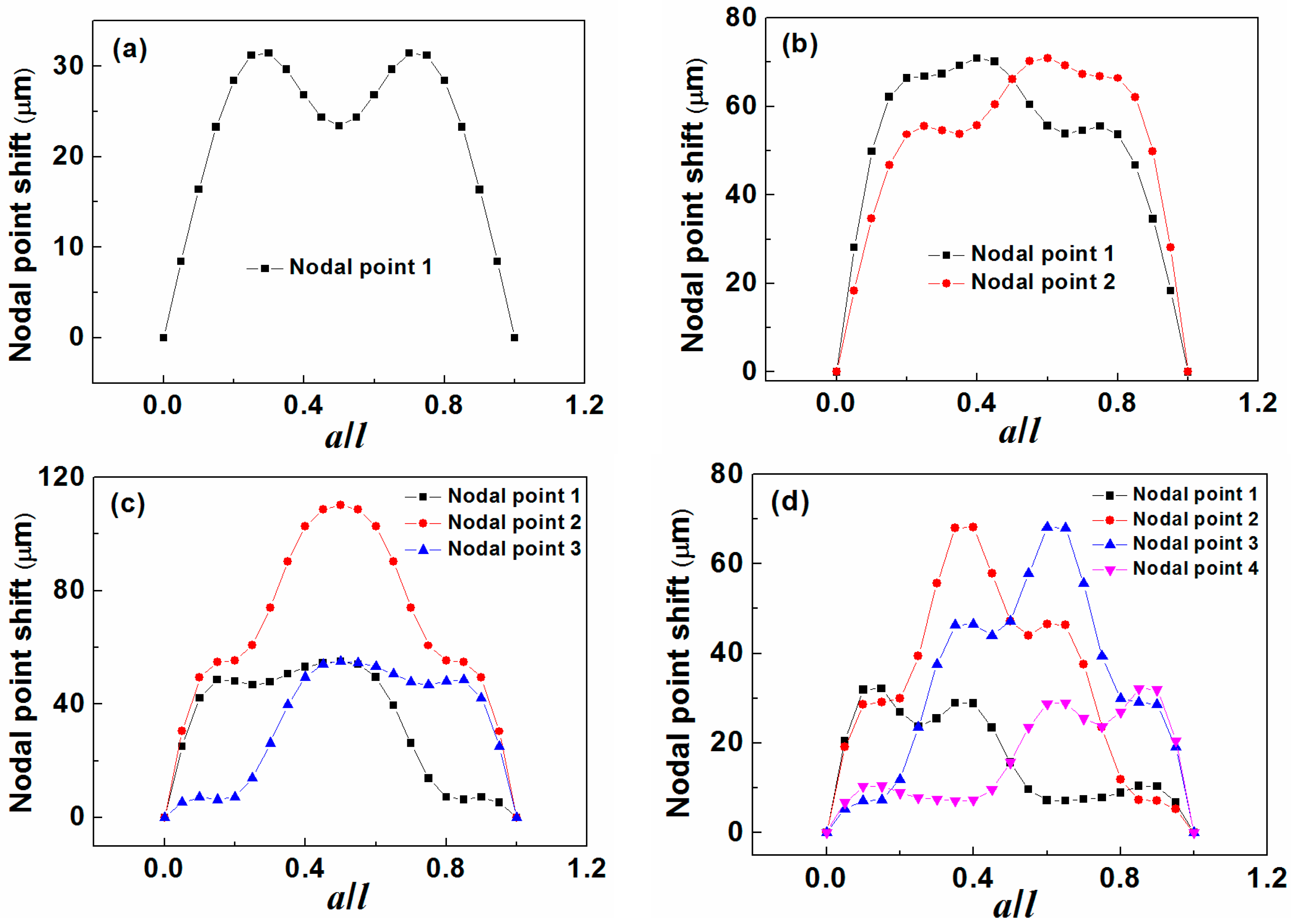
3.1. The Effect on Motion Patterns and “Nodal Points”

| Resonance Order | Nodal Point Position(s) at x = |
|---|---|
| 1 | l/2 |
| 2 | l/4, 3l/4 |
| 3 | l/6, l/2, 5l/6 |
| 4 | l/8, 3l/8, 5l/8, 7l/8 |

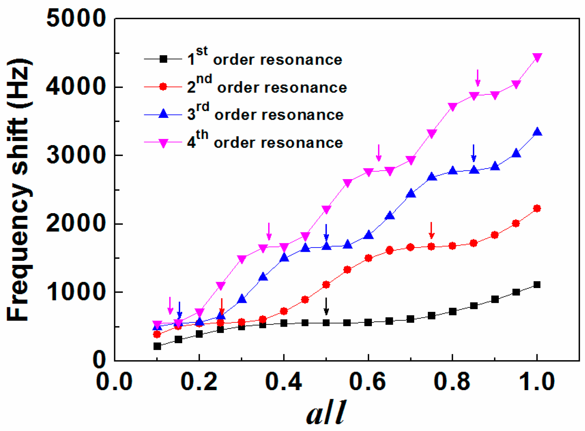
3.2. The Effect on Frequency Shift

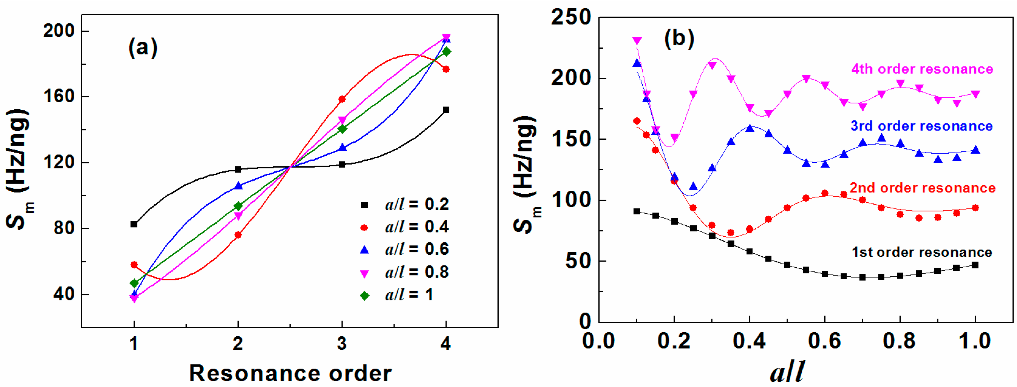
3.3. The Effect on Mass Sensitivity
| Resonance Order | Mass Sensitivity (Hz/ng) | |
|---|---|---|
| Methodology Used in This Study | Equations (8) and (9) | |
| 1 | 47 | 47 |
| 2 | 94 | 94 |
| 3 | 141 | 141 |
| 4 | 188 | 188 |


4. Conclusions
- The motion pattern of a magnetoelastic sensor is dependent on its resonance mode and the mass load distribution. The mass sensitivity and “nodal point” position are related to the point displacement, which is determined by the motion pattern. Asymmetrical mass load distribution causes the motion patterns lose symmetry and leads to the shift in “nodal point”.
- For any one odd-order resonance mode (2n − 1, n = 1, 2, 3, … ), there is always one curve((n)th “nodal point”) self-symmetrical about a/l = 0.5 and (n − 1) pair of curves((q)th “nodal point” and (2n − q)th “nodal point” where q = 1, 2, 3, …, n − 1) mirror-symmetrical about a/l = 0.5 while for even-order (2m, m = 1, 2, 3, … ) resonance mode, there are only m pair of curves((p + 1)th “nodal point” and (2m − p)th “nodal point” where p = 0, 1, 2, …, m − 1) mirror-symmetrical about a/l = 0.5.
- Mass loaded near the “nodal point” has little contribution on the resonance frequency shift as well as the mass sensitivity.
- Mass sensitivity linearly increases with resonance order for symmetrical mass load distribution but nonlinearly varies for asymmetrical mass load distribution, which is attributed to the loss of symmetry of motion patterns.
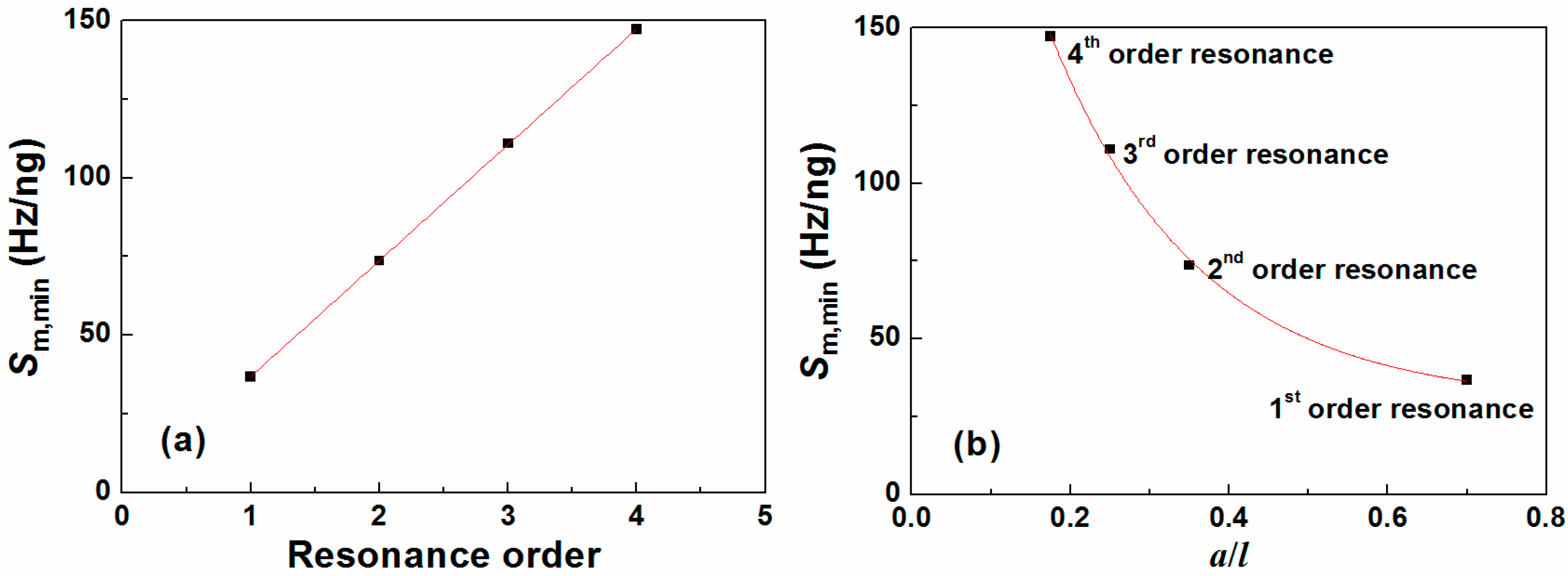
- The mass sensitivity as the function of a/l behaves like sine waves with decaying amplitude. The minimum mass sensitivity appears at the first valley and is linearly proportional to the resonance order.
Acknowledgments
Author Contributions
Conflicts of Interest
References
- Grimes, C.A.; Mungle, C.S.; Zeng, K.F.; Jain, M.K.; Dreschel, W.R.; Paulose, M.; Ong, K.G. Wireless magnetoelastic resonance sensors: A critical review. Sensors 2002, 2, 294–313. [Google Scholar] [CrossRef]
- Zhang, K.W.; Zhang, L.; Fu, L.L.; Li, S.Q.; Chen, H.Q.; Cheng, Z.Y. Magnetostrictive resonators as sensors and actuators. Sens. Actuators A Phys. 2013, 200, 2–10. [Google Scholar] [CrossRef]
- Zhang, K.W.; Fu, L.L.; Zhang, L.; Cheng, Z.Y.; Huang, T.S. Magnetostrictive particle based biosensors for in situ and real-time detection of pathogens in water. Biotechnol. Bioeng. 2014, 111, 2229–2238. [Google Scholar] [CrossRef] [PubMed]
- Park, M.K.; Li, S.Q.; Chin, B.A. Detection of Salmonella Typhimurium Grown Directly on Tomato Surface Using Phage-Based Magnetoelastic Biosensors. Food Bioprocess Technol. 2013, 6, 682–689. [Google Scholar] [CrossRef]
- Li, S.Q.; Li, Y.G.; Chen, H.Q.; Horikawa, S.; Shen, W.; Simonian, A.; Chin, B.A. Direct detection of Salmonella typhimurium on fresh produce using phage-based magnetoelastic biosensors. Biosens. Bioelectron. 2010, 26, 1313–1319. [Google Scholar] [CrossRef] [PubMed]
- Lakshmanan, R.S.; Guntupalli, R.; Hu, J.; Petrenko, V.A.; Barbaree, J.M.; Chin, B.A. Detection of Salmonella typhimurium in fat free milk using a phage immobilized magnetoelastic sensor. Sens. Actuators B Chem. 2007, 126, 544–550. [Google Scholar] [CrossRef]
- Guntupalli, R.; Hu, J.; Lakshmanan, R.S.; Huang, T.S.; Barbaree, J.M.; Chin, B.A. A magnetoelastic resonance biosensor immobilized with polyclonal antibody for the detection of Salmonella typhimurium. Biosens. Bioelectron. 2007, 22, 1474–1479. [Google Scholar] [CrossRef] [PubMed]
- Huang, S.C.; Yang, H.; Lakshmanan, R.S.; Johnson, M.L.; Wan, J.H; Chen, I.H.; Wikle, H.C.; Petrenko, V.A.; Barbaree, J.M.; Chin, B.A. Sequential detection of Salmonella typhimurium and Bacillus anthracis spores using magnetoelastic biosensors. Biosens. Bioelectron. 2009, 24, 1730–1736. [Google Scholar] [CrossRef] [PubMed]
- Chai, Y.T.; Li, S.Q.; Horikawa, S.; Park, M.K.; Vodyanoy, V.; Chin, B.A. Rapid and sensitive detection of Salmonella Typhimurium on eggshells by using wireless biosensors. J. Food Protect. 2012, 75, 631–636. [Google Scholar] [CrossRef] [PubMed]
- Johnson, M.L.; Wan, J.H.; Huang, S.C.; Cheng, Z.Y.; Petrenko, V.A.; Kim, D.J.; Chen, I.H.; Barbaree, J.M.; Hong, J.W.; Chin, B.A. A wireless biosensor using microfabricated phase-interfaced magnetoelastic particles. Sens. Actuators A Phys. 2008, 144, 38–47. [Google Scholar] [CrossRef]
- Shen, W.; Lakshmanan, R.S.; Mathison, L.C.; Petrenko, V.A.; Chin, B.A. Phage coated magnetoelastic micro-biosensors for real-time detection of Bacillus anthracis spores. Sens. Actuators B Chem. 2009, 137, 501–506. [Google Scholar] [CrossRef]
- Hiremath, N.; Guntupalli, R.; Vodyanoy, V.; Chin, B.A.; Park, M.K. Detection of methicillin-resistant Staphylococcus aureus using novellytic phage-based magnetoelastic biosensors. Sens. Actuators B Chem. 2015, 210, 129–136. [Google Scholar] [CrossRef]
- Kouzoudis, D.; Baimpos, T.; Nikolakis, V. Detection of hazardous VOCs using a zeolite FAU/Metglas magnetoelastic sensor. Procedia Eng. 2011, 25, 1621–1624. [Google Scholar] [CrossRef]
- Ong, K.G.; Paulose, M.; Jain, M.K.; Gong, D.; Varghese, O.K.; Mungle, C.; Grimes, C.A. Magnetism-based remote query glucose sensors. Sensors 2001, 1, 138–147. [Google Scholar] [CrossRef]
- Zhang, R.; Tejedor, M.I.; Anderson, M.A.; Paulose, M.; Grimes, C.A. Ethylene detection using nanoporous PtTiO2 coatings appliedto magnetoelastic thick films. Sensors 2002, 2, 331–338. [Google Scholar] [CrossRef]
- Li, S.Q.; Cheng, Z.Y. Nonuniform mass detection using magnetostrictive biosensors operating under multiple harmonic resonance modes. J. Appl. Phys. 2010, 107, 114514. [Google Scholar] [CrossRef]
- Cheng, Z.Y.; Li, S.Q.; Zhang, K.W.; Fu, L.L.; Chin, B.A. Novel magnetostrictive microcantilever and magnetostrictive nanobars for high performance biological detection. Adv. Sci. Tech. 2008, 54, 19–28. [Google Scholar] [CrossRef]
- Ramasamy, M.; Liang, C.; Prorok, B.C. Magneto-mechanical mems sensors for bio-detection. In MEMS and Nanotechnology, Proceedings of the SEM Annual Conference; Springer: New York, NY, USA, February 2011; pp. 9–15. [Google Scholar]
- Zhang, K.W.; Zhang, K.H.; Chai, Y.S. Study of “blind point” and mass sensitivity of a magnetostrictive biosensor with asymmetric mass loading. AIP Adv. 2014, 4, 057114. [Google Scholar] [CrossRef]
- Li, S.Q.; Fu, L.L.; Barbaree, J.M.; Cheng, Z.Y. Resonance behavior of magnetostrictive micro/milli-cantilever and itsapplication as a biosensor. Sens. Actuators B Chem. 2009, 137, 692–699. [Google Scholar] [CrossRef]
- Fu, L.L.; Zhang, K.W.; Li, S.Q.; Wang, Y.H.; Huang, T.S.; Zhang, A.X.; Cheng, Z.Y. In situ real-time detection of E. coli in water using antibody-coatedmagnetostrictive microcantilever. Sens. Actuators B Chem. 2010, 150, 220–225. [Google Scholar] [CrossRef]
- Johnson, B.N.; Mutharasan, R. A novel experimental technique for determining node location in resonant mode cantilevers. J. Micromech. Microeng. 2011, 21, 065027. [Google Scholar] [CrossRef]
- Johnson, B.N.; Mutharasan, R. The origin of low-order and high-order impedance-coupled resonant modes in piezoelectric-excited millimeter-sized cantilever (PEMC) sensors: Experiments and finite element models. Sens. Actuators B Chem. 2011, 155, 868–877. [Google Scholar] [CrossRef]
- Muraoka, M. Sensitivity-enhanced atomic force acoustic microscopy with concentrated-mass cantilevers. Nanotechnology 2005, 16, 542. [Google Scholar] [CrossRef]
- Dohn, S.; Svendsen, W.; Boisen, A.; Hansen, O. Mass and position determination of attached particles on cantilever based mass sensors. Rev. Sci. Instrum. 2007, 78, 103303. [Google Scholar] [CrossRef] [PubMed]
- Ballantine, D.S.; White, R.M.; Martin, S.J.; Ricco, A.J.; Frye, G.C.; Zellers, E.T.; Wohltjen, H. Acoustic Wave Sensors: Theory, Design and Physico-Chemical Applications; Academic press: New York, NY, USA, 1997. [Google Scholar]
- Metglas. Available online: http://www.metglas.com (accessed on 11 August 2015).
- Liang, C.; Morshed, S.; Prorok, B.C. Correction for longitudinal mode vibration in thin slender beams. Appl. Phys. Lett. 2007, 90, 221912. [Google Scholar] [CrossRef]
© 2015 by the authors; licensee MDPI, Basel, Switzerland. This article is an open access article distributed under the terms and conditions of the Creative Commons Attribution license (http://creativecommons.org/licenses/by/4.0/).
Share and Cite
Zhang, K.; Zhang, L.; Chai, Y. Mass Load Distribution Dependence of Mass Sensitivity of Magnetoelastic Sensors under Different Resonance Modes. Sensors 2015, 15, 20267-20278. https://doi.org/10.3390/s150820267
Zhang K, Zhang L, Chai Y. Mass Load Distribution Dependence of Mass Sensitivity of Magnetoelastic Sensors under Different Resonance Modes. Sensors. 2015; 15(8):20267-20278. https://doi.org/10.3390/s150820267
Chicago/Turabian StyleZhang, Kewei, Lin Zhang, and Yuesheng Chai. 2015. "Mass Load Distribution Dependence of Mass Sensitivity of Magnetoelastic Sensors under Different Resonance Modes" Sensors 15, no. 8: 20267-20278. https://doi.org/10.3390/s150820267