
Review of Trackside Monitoring Solutions: From Strain Gages to Optical Fibre Sensors


Abstract
:1. Introduction

2. Static and Dynamic Behaviour of Ballasted Railway Tracks

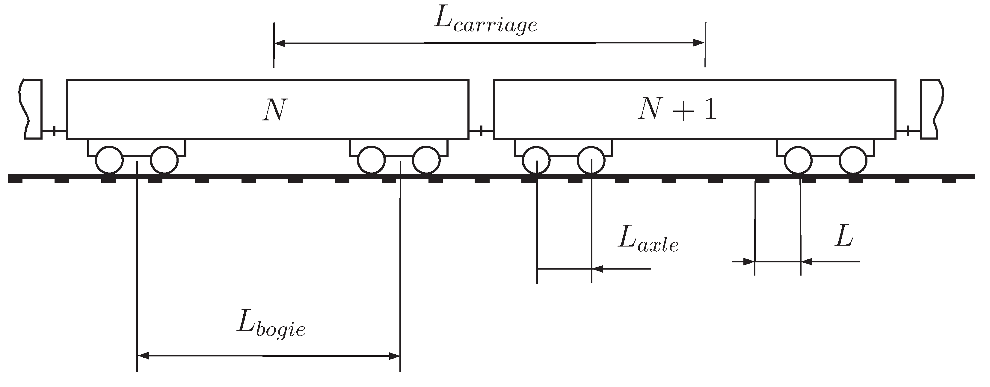
- Related to the vehicle, the suspensions (primary and secondary), carbody, bogie and wheelset masses play an important role in the vehicle vibration modes.
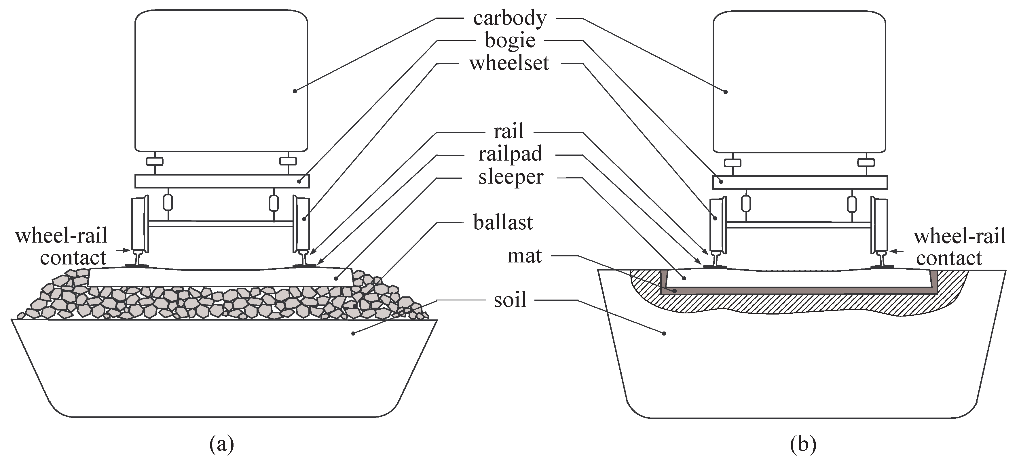
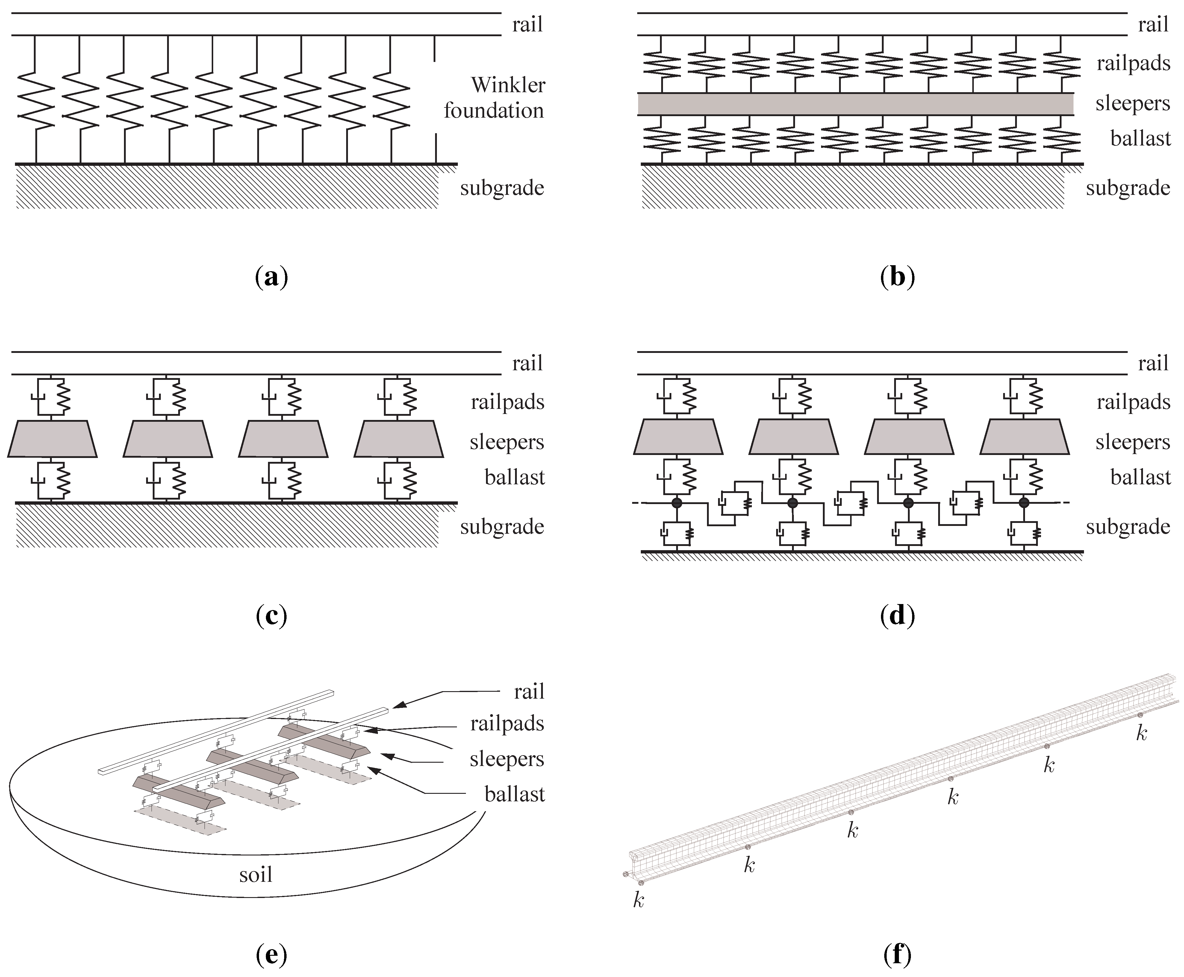
- Related to the track, various rail profiles and types are available in the railway transport, according to the form, the weight and the track nature. It is noticeable that the standard steel used it typically constant (Young’s modulus: and density: ). Additionally the geometry varies according to the application and the country. The role of the railpads is to absorb a part of rail vibrations and to allow the wheel to traverse the rail, without damaging the sleeper. The sleeper is another important constitutive element of the track. It has two main roles: to transfer the loads from the rails to the track ballast (or mat) and the ground underneath, meanwhile maintaining the rail gauge. Ballast is used to facilitate the drainage of water and to distribute the load from the railroad ties/sleepers, without distortion by settlement. Ballasted and non-ballasted tracks present similar vertical dynamic behaviour [13]. Therefore, only ballasted railway tracks are considered in the present study.
- Related to the soil, the dynamic response of foundations subjected to dynamic loadings depends on some key parameters (soil profiles, foundation form and geometry, interaction between adjacent foundations, …) with amplifications and/or attenuations as a function of the excitation frequency [14]. influencing the response.
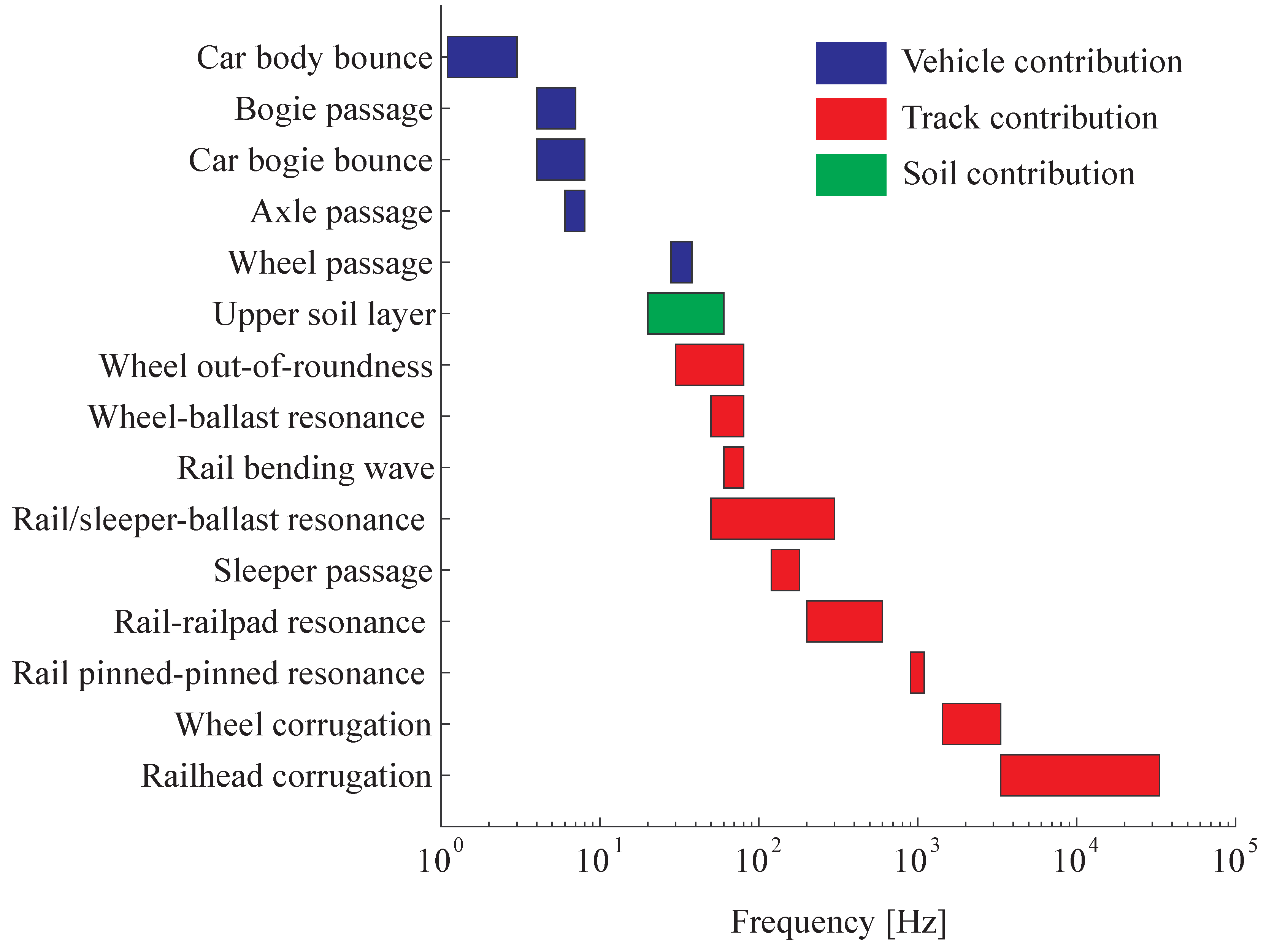
- Vehicle dynamics intervene in the low-frequency range (until ) and are efficiently transmitted to the ground if significant defects in the wheel/rail contact excite the vehicle natural modes.
- Mid range frequencies (from to ) are due to the track flexibility with possible amplification due to the soil resonance.
- High-frequencies (over ) constitute rolling noise due to the wheel/rail sliding and rarely intervene in the ground vibrations because the soil strongly absorbs the vibrations (material and geometrical damping).

- The vehicle dynamics can amplify the spectrum at low frequencies where the vehicle modes interact with the track when rolling on non-perfect surfaces (distributed unevenness or local defect like turnouts and wheel flats). This may amplify the excitation passages frequencies.
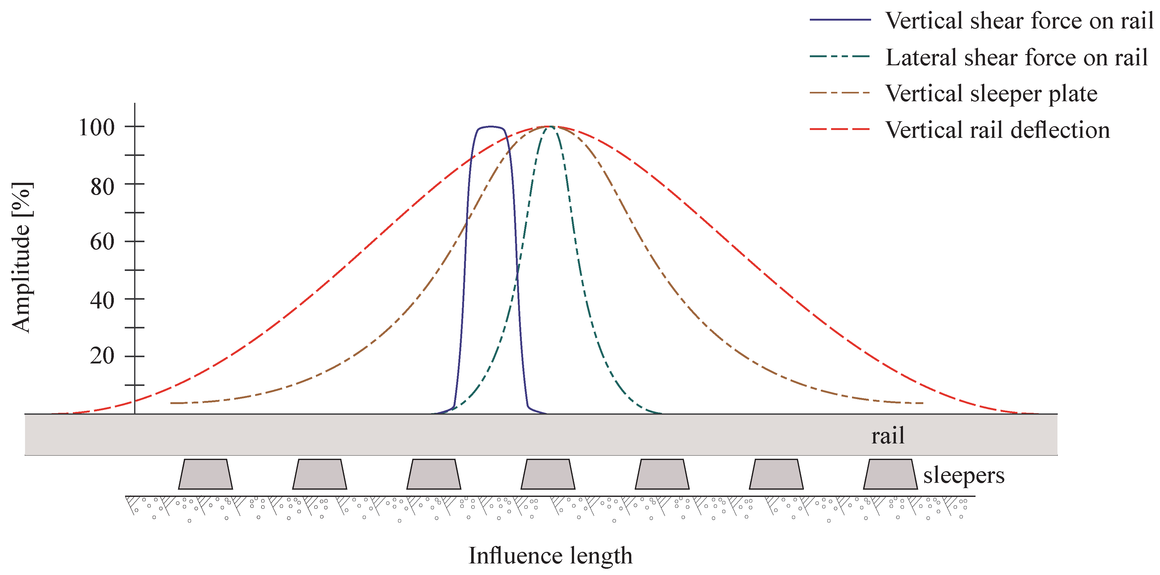
- The vertical track dynamics is mainly affected by three resonances: a first resonance where the rail and sleepers vibrate vertically in phase (typically at a frequency around 50–), a second resonance where rail and sleepers vibrate out of phase (at a medium frequency in the range 200–) and a third mode, called the pinned-pinned resonance, where the rail vibrates with a wavelength equal to two sleeper bays (close to 800–).
- The ground provides two kinds of attenuation: geometric damping and material soil damping. This refers to the exponential decrease of vibration magnitude with distance and to an attenuation at high-frequencies, respectively. Moreover, if the ground is considered as a superposition of layers with different dynamic properties, a resonance can appear if the difference in rigidity between the two top layers is significant and the excitation acts in the vertical direction [19]. The corresponding frequency can be approximated by [20]with the soil longitudinal wave velocity and h the depth of the soil first layer. Practically, this resonance occurs in a frequency range between 20 and depending on the site configuration. This mode is highly damped, meaning that the resonance area covers a large frequency band.
- In practice, rail and wheel surface imperfections (distributed rail and wheel unevenness, roughness of the wheel and rail surface, out-of-roundness of the wheel, wheel flat, wheel seized ball bearing and other singular track defect like switches, crossings and rail joints) shape up the wheel/rail forces, introducing a fluctuation around the static value.
3. Estimation of Rail Stress and Monitoring Assessment Using Numerical Models


4. Typical Sensor Configurations

- Contacting displacement transducers like LVDT yield a relative motion because of how they are mounted. They have a limited frequency bandwidth (modern LVDTs have a usable bandwidth from 0 to [49]) and may be not suitable for some applications where the frequencies of interest are outside this range. They also need to be calibrated during installation.
- Non-contacting transducers like capacitance-type transducers present excellent stability and repeatability and require little maintenance. However, a particular attention should be paid to their calibration to assure proper linearity and sensitivity. They are also sensitive to electrical noise and to temperature.
- Most often, a specific and dedicated mounting arrangement is necessary, which complicates installation.

| Contributing Parameters | Requirements/Limitations | |
|---|---|---|
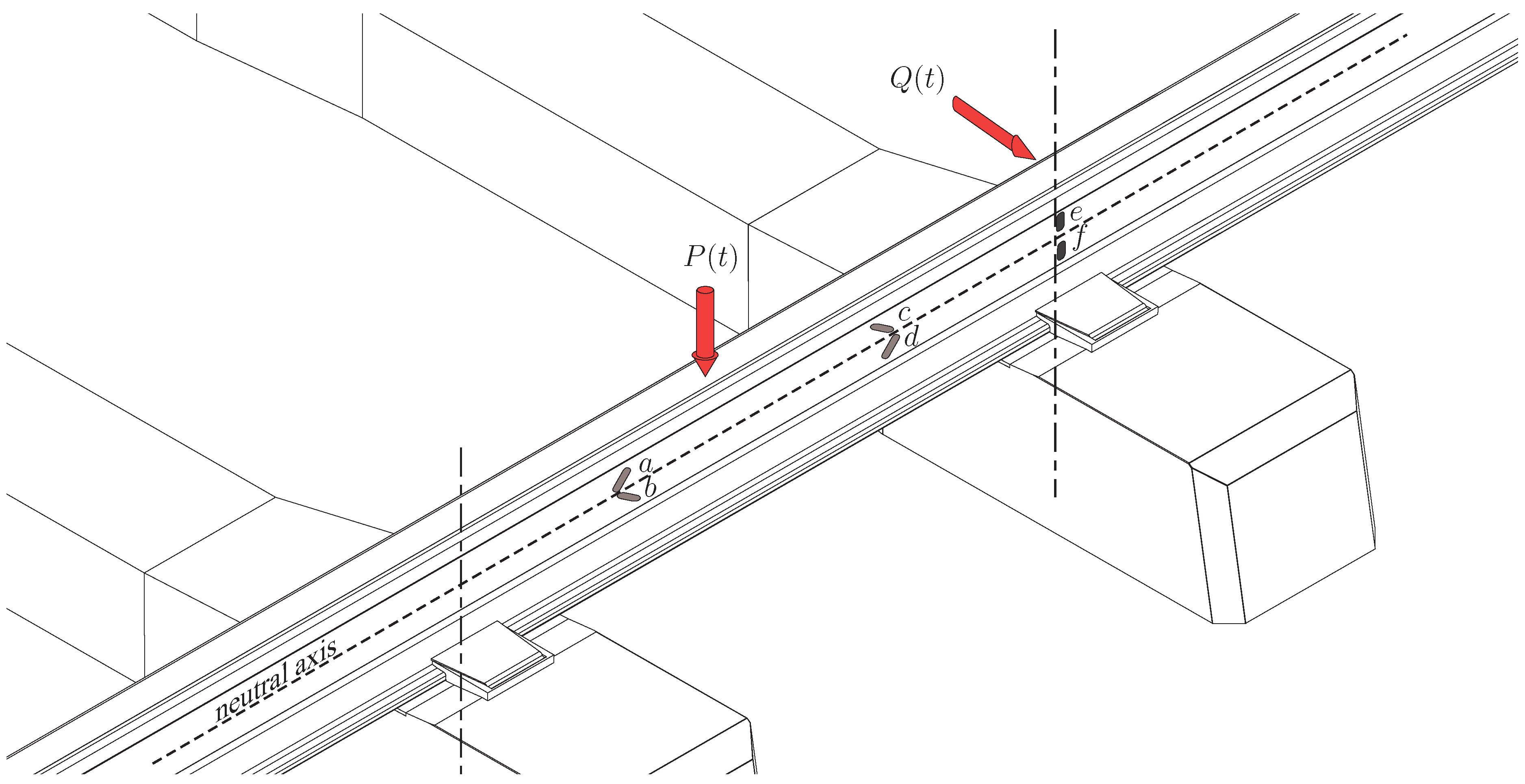
| Strain gage | Wheel/rail force | Accurate positioning (neutral axis) |
| Vehicle position | Sensitive to electromagnetic interferences | |
| Difficulty of gluing and/or soldering | ||
| (except waterproof or embedded sensor systems) | ||
| Accelerometers | Track deflection | Absolute motion |
| Vehicle position | Sensitive to external excitation | |
| Specific signal processing | ||
| Geophones | Track deflection | Absolute motion |
| Vehicle position | Sensitive to external excitation | |
| Limited frequency range | ||
| LVDT | Track deformation | Specific mounting |
| Limited frequency range | ||
| MDD | Foundation deflections | Specific installation |
5. Using Optical Fibre-Based Sensors as an Alternative
| Transduction Mechanism | Sensor Location | Sensor Fixation | Spatial Resolution | |
|---|---|---|---|---|
| Bragg | Axial strain induces a Bragg wavelength shift | On the rail or on the sleeper | With glue, screws, welding or with dedicated magnetic or mechanical patch | Quasi-distributed sensing (maximum 50 gratings per channel |
| Brillouin | Axial strain induces a shift of the Brillouin frequency | On the rail | With glue | Distributed sensing (≈) |
| Acoustic | Acoustic pressure induces a change of the Rayleigh backscatter intensity | On the rail, close to the rail or even buried | With glue if on the rail | Distributed sensing (≈) |
6. Discussion and Useful Guidance
- The utility of a prediction model has been pointed out in order to assess the optimal positioning and orientation of sensors. Increasing the complexity of a numerical model goes hand in hand with the need for more track parameters (e.g., railpad, sleeper or foundation behaviour) and an increase of computational burden, which often limit the analysis to simple cases.
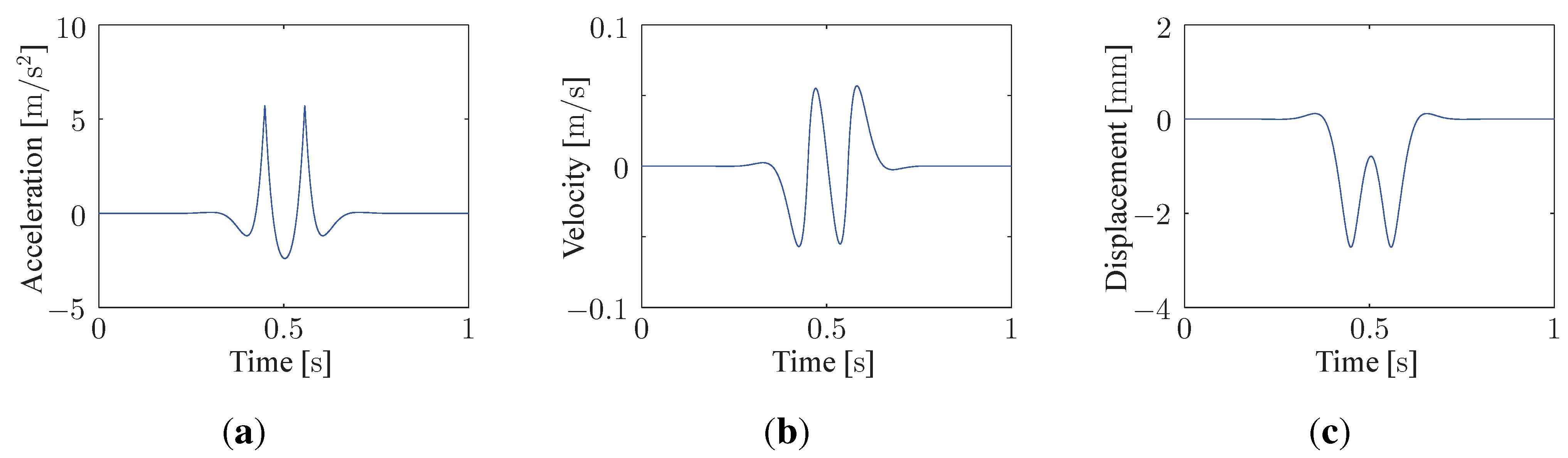
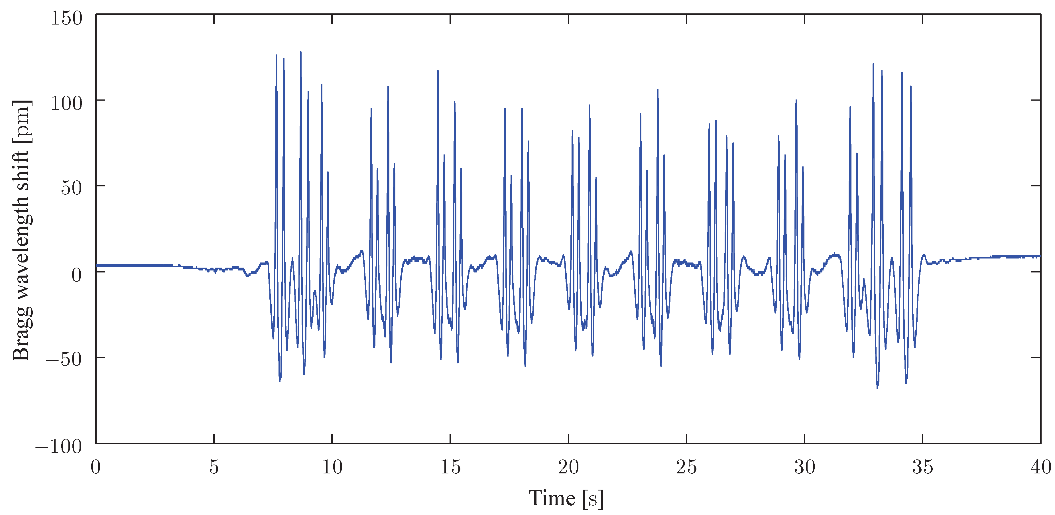
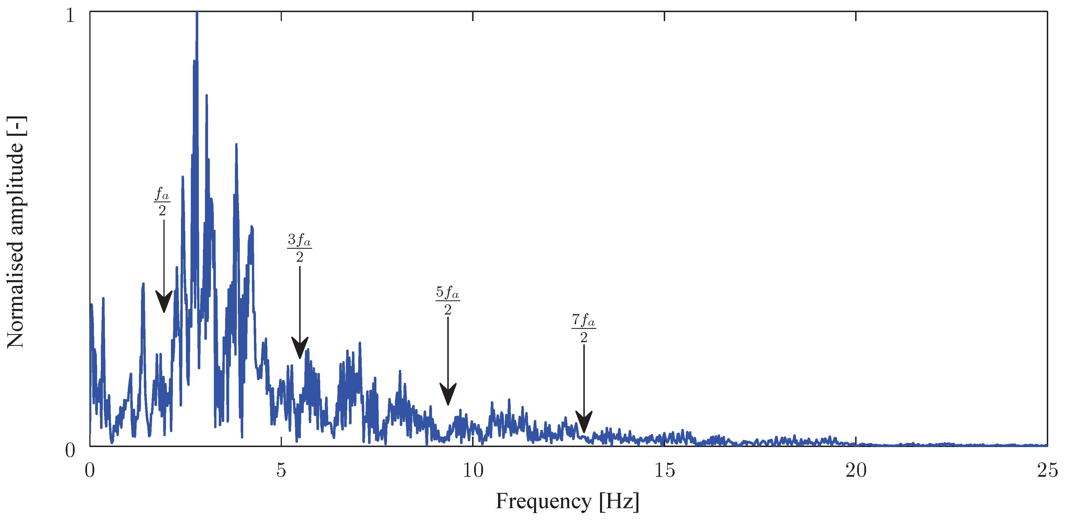
- The knowledge of track dynamics allows the understanding of some specific phenomena. For example, the spectral analysis of the recorded time history presented in Figure 13 is plotted in Figure 14. The expected information is ranged between 0 and due to the low vehicle speed (). As described in Section 2, an amplitude modulation is clearly visible and some information can be deduced from these periodicities (for example, at frequencies , the amplitude tends towards zero).
- Some important requirements for classical sensors (strain gauges) can be used as a guidance for the positioning of fibre-based sensors and the analysis of resulting signals. Position and orientation can be borrowed from the experience of strain gauges and applied to fibre sensor measuring the local deformation.
- The mounting of the sensors is also of great importance. Although cementing and screwing are the most commonly adopted solution, other mountings (welding, magnetic attaching, clamping, …) are also of interest. It appears that there is no universal solution for sensor packaging but some precautions and requirements must be taken: a correct strain transfer (rail polishing in the case of gluing), an ease of installation, a minimum of robustness towards weather and resistance to rail maintenance, a replacement without damaging the sensor, …
- A high reliability is required in railway industry, according to IEC 61508 [75] and IEC 62279 [76] standards (IEC 62279 provides a specific interpretation of IEC 61508 for railway applications). A risk assessment effort yields a target safety integrity level (SIL) with an expected probability of failure per hour less than (SIL4, which is the most dependable, has become a requirement in railway to attain in regards to a system’s development).
7. Conclusions
Acknowledgments
Conflicts of Interest
References
- Ghazel, M. Formalizing a subset of ERTMS/ETCS specifications for verification purposes. Transp. Res. Part C Emerg. Technol. 2014, 42, 60–75. [Google Scholar] [CrossRef]
- FP7 European project ACEM-Rail—Automated and Cost Effective Railway Infrastructure Maintenance (FP7-SST-2010-RTD-1). Available online: http://www.acem-rail.eu (accessed on 9 May 2015).
- Ni, S.H.; Huang, Y.H.; Lo, K.F. An automatic procedure for train speed evaluation by the dominant frequency method. Comput. Geotech. 2011, 38, 416–422. [Google Scholar] [CrossRef]
- Bowness, D.; Lock, A.C.; Powrie, W.; Priest, J.A.; Richards, D.J. Monitoring the dynamic displacements of railway track. J. Rail Rapid Transit 2007, 221, 13–22. [Google Scholar] [CrossRef]
- Murray, C.A.; Take, W.A.; Hoult, N.A. Measurement of vertical and longitudinal rail displacements using digital image correlation. Can. Geotech. J. 2015, 52, 141–155. [Google Scholar] [CrossRef]
- Gräbe, P.J.; Shaw, F.J. Design life prediction of a heavy haul track foundation. J. Rail Rapid Transit 2010, 224, 33–344. [Google Scholar] [CrossRef]
- Pinto, N.; Ribeiro, C.A.; Gabriel, J.; Calçada, R. Dynamic monitoring of railway track displacement using an optical system. J. Rail Rapid Transit 2015, 229, 280–290. [Google Scholar] [CrossRef]
- Udd, E. An overview of fiber-optic sensors. Rev. Sci. Instrum. 1995, 66, 4015–4030. [Google Scholar] [CrossRef]
- Luyckx, G.; Voet, E.; Lammens, N.; Degrieck, J. Strain measurements of composite laminates with embedded fibre Bragg gratings: Criticism and opportunities for research. Sensors 2011, 11, 384–408. [Google Scholar] [CrossRef] [PubMed] [Green Version]
- Kinet, D.; Mégret, P.; Goossen, K.W.; Qiu, L.; Heider, D.; Caucheteur, C. Fiber Bragg Grating sensors toward structural health monitoring in composite materials: Challenges and solutions. Sensors 2014, 14, 7394–7419. [Google Scholar] [CrossRef] [PubMed]
- Ye, X.W.; Su, Y.H.; Han, J.P. Structural health monitoring of civil infrastructure using optical fiber sensing technology: A comprehensive review. Sci. World J. 2014, 652329. [Google Scholar] [CrossRef] [PubMed]
- Kurzych, A.; Jaroszewicz, L.R.; Krajewski, Z.; Teisseyre, K.P.; Kowalski, J.K. Fibre optic system for monitoring rotational seismic phenomena. Sensors 2014, 14, 5459–5469. [Google Scholar] [CrossRef] [PubMed]
- Knothe, K.; Grassie, S.L. Modelling of railway track and vehicle/track interaction at high frequencies. Veh. Syst. Dyn. 1993, 22, 209–262. [Google Scholar] [CrossRef]
- Gazetas, G. Analysis of machine foundation vibrations: state of the art. Soil Dyn. Earthq. Eng. 1983, 2, 2–42. [Google Scholar] [CrossRef]
- Alias, J. La Voie Ferrée—Technique de Construction et D’entretien; Eyrolles: Paris, France, 1984. [Google Scholar]
- Ju, S.H.; Lin, H.T.; Huang, J.Y. Dominant frequencies of train-induced vibrations. J. Sound Vib. 2009, 319, 247–259. [Google Scholar] [CrossRef]
- Kouroussis, G.; Connolly, D.P.; Vogiatzis, K.; Verlinden, O. Modelling the environmental effects of railway vibrations from different types of rolling stock—A numerical study. Shock Vib. 2015, 2015, 142807. [Google Scholar] [CrossRef]
- Kouroussis, G.; Connolly, D.P.; Verlinden, O. Railway induced ground vibrations—A review of vehicle effects. Int. J. Rail Transp. 2014, 2, 69–110. [Google Scholar] [CrossRef]
- Kouroussis, G.; Conti, C.; Verlinden, O. Investigating the influence of soil properties on railway traffic vibration using a numerical model. Veh. Syst. Dyn. 2013, 51, 421–442. [Google Scholar] [CrossRef]
- Kramer, S.L. Geotechnical Earthquake Engineering; Prentice–Hall: Upper Saddle River, NJ, USA, 1996. [Google Scholar]
- Connolly, D.P.; Kouroussis, G.; Laghrouche, O.; Ho, C.; Forde, M.C. Benchmarking railway vibrations—Track, vehicle, ground and building effects. Constr. Build. Mater. 2015, 92, 64–81. [Google Scholar] [CrossRef]
- Grassie, S.L.; Gregory, R.W.; Harrison, D.; Johnson, K.L. The dynamic response of railway track to high frequency vertical excitation. J. Mech. Eng. Sci. 1982, 24, 77–90. [Google Scholar] [CrossRef]
- Grassie, S.L. Models of railway track and vehicle/track interaction at high frequencies: Results of Benchmark test. Veh. Syst. Dyn. 1996, 25, 243–262. [Google Scholar] [CrossRef]
- Timoshenko, S. On the transverse vibrations of bars of uniform cross-section. Philos. Mag. Ser. 6 1922, 43, 125–131. [Google Scholar] [CrossRef]
- Tutumluer, E.; Qian, Y.; Hashash, Y.M.A.; Ghaboussi, J.; Davis, D.D. Discrete element modelling of ballasted track deformation behaviour. Int. J. Rail Transp. 2013, 1, 57–73. [Google Scholar] [CrossRef]
- Zhai, W.; Sun, X. A detailled model for investigating vertical interaction between railway vehicle and track. Veh. Syst. Dyn. 1994, 23, 603–615. [Google Scholar] [CrossRef]
- Patil, S.P. Natural frequencies of a railroad track. J. Appl. Mech. 1987, 54, 299–304. [Google Scholar] [CrossRef]
- Cai, Y.; Cao, Z.; Sun, H.; Xu, C. Effects of the dynamic wheel-rail interaction on the ground vibration generated by a moving train. Int. J. Solids Struct. 2010, 47, 2246–2259. [Google Scholar] [CrossRef]
- Oscarsson, J.; Dahlberg, T. Dynamic train/track/ballast interaction—Computer models and full-scale experiments. Veh. Syst. Dyn. 1998, 29, 73–84. [Google Scholar] [CrossRef]
- Knothe, K.; Wu, Y. Receptance behaviour of railway track and subgrade. Arch. Appl. Mech. 1998, 68, 457–470. [Google Scholar] [CrossRef]
- Kouroussis, G.; Gazetas, G.; Anastasopoulos, I.; Conti, C.; Verlinden, O. Discrete modelling of vertical track–soil coupling for vehicle–track dynamics. Soil Dyn. Earthq. Eng. 2011, 31, 1711–1723. [Google Scholar] [CrossRef]
- Nielsen, J.C.O.; Abrahamsson, T.J.S. Coupling of physical and modal components for analysis of moving non-linear dynamic systems on general beam structures. Int. J. Numer. Methods Eng. 1992, 33, 1843–1859. [Google Scholar] [CrossRef]
- Andersson, C.; Oscarsson, J. Dynamic train/track interaction including state-dependent track properties and flexible vehicle components. Veh. Syst. Dyn. 1999, 33, 47–58. [Google Scholar]
- Uzzal, R.U.A.; Ahmed, W.; Bhat, R.B. A three-dimensional modeling study of wheel/rail impacts created by multiple wheel flats, and the development of a smart wheelset. J. Rail Rapid Transit 2014. [Google Scholar] [CrossRef]
- Grossoni, I.; Iwnicki, S.; Bezin, Y.; Gong, C. Dynamics of a vehicle–track coupling system at a rail joint. J. Rail Rapid Transit 2014, 229, 364–374. [Google Scholar] [CrossRef]
- Zhao, X.; Li, Z.; Liu, J. Wheel–rail impact and the dynamic forces at discrete supports of rails in the presence of singular rail surface defects. J. Rail Rapid Transit 2012, 226, 124–139. [Google Scholar] [CrossRef]
- Zhai, W.; Wang, S.; Zhang, N.; Gao, M.; Xia, H.; Cai, C.; Zhao, C. High-speed train–track–bridge dynamic interactions—Part II: experimental validation and engineering application. Int. J. Rail Transp. 2013, 1, 25–41. [Google Scholar] [CrossRef]
- Arvidsson, T.; Karoumi, R. Train–bridge interaction—A review and discussion of key model parameters. Int. J. Rail Transp. 2014, 2, 147–186. [Google Scholar] [CrossRef]
- Stow, J.; Andersson, E. Field testing and instrumentation of railway vehicles. In Handbook of Railway Vehicle Dynamics; Iwnicki, S., Ed.; CRC Press: New York, NY, USA, 2006. [Google Scholar]
- Ahlbeck, D.R.; Harrison, H.D.; Prause, R.H.; Johnson, M.R. Evaluation of Analytical and Experimental Methodologies for the Characterization of Wheel/Rail Loads; National Institute of Standards and Technology (U.S.), Department of Transportation, Federal Railroad Administration, Office of Research and Development: Washington, DC, USA, 1976.
- Askarinejad, H.; Dhanasekar, M.; Colel, C. Assessing the effects of track input on the response of insulted rail joins using field experiments. J. Rail Rapid Transit 2012, 227, 176–187. [Google Scholar] [CrossRef]
- Palo, M.; Galar, D.; Nordmark, T.; Asplund, M.; Larsson, D. Condition monitoring at the wheel/rail interface for decision-making support. J. Rail Rapid Transit 2014. [Google Scholar] [CrossRef]
- Milković, D.; Simić, G.; Jakovljević, Z̆.; Tanasković, J.; Luc̆anin, V. Wayside system for wheel-rail contact forces measurements. Measurement 2013, 46, 3308–3318. [Google Scholar] [CrossRef]
- Ahmad, S.S.; Mandal, N.K.; Chattopadhyay, G.; Powell, J. Development of a unified railway track stability management tool to enhance track safety. J. Rail Rapid Transit 2013, 227, 493–516. [Google Scholar] [CrossRef]
- Delprete, C.; Rosso, C. An easy instrument and a methodology for the monitoring and the diagnosis of a rail. Mech. Syst. Signal Process. 2009, 23, 940–956. [Google Scholar] [CrossRef]
- Molatefi, H.; Mozafari, H. Analysis of new method for vertical load measurement in the barycenter of the rail web by using FEM. Measurement 2013, 46, 2313–2323. [Google Scholar] [CrossRef]
- Ryjác̆ek, P.; Vokác̆, M. Long-term monitoring of steel railway bridge interaction with continuous welded rail. J. Constr. Steel Res. 2014, 99, 176–186. [Google Scholar] [CrossRef]
- Brincker, L.; Lagö, T.L.; Andersen, P.; Ventura, C. Improving the classical geophone sensor element by digital correction. In Proceedings of IMAC-XXIII: A Conference & Exposition on Structural Dynamics, Orlando, FL, USA, 31 January–3 February 2005.
- Harris, C.M. (Ed.) Shock and Vibration Handbook, 6th ed.; McGraw–Hill: New York, NY, USA, 2009.
- Bennett, G.J.; Antunes, J.; Fitzpatrick, J.A.; Debut, V. A method for optimal reconstruction of velocity response using experimental displacement and acceleration signals. In Proceedings of the 14th International Congress on Sound and Vibration (ICSV14), Cairns, Australia, 9–12 July 2007.
- Brandt, A. Noise and Vibration Analysis: Signal Analysis and Experimental Procedures; John Wiley & Sons: West Sussex, UK, 2011. [Google Scholar]
- Lamas-Lopez, F.; Alves-Fernandes, V.; Cui, Y.J.; D’Aguiar, S.C.; Calon, N.; Canou, J.; Dupla, J.; Tang, A.; Robinet, A. Assessment of the double integration method using accelerometers data for conventional railway platforms. In Proceedings of the Second International Conference on Railway Technology: Research, Development and Maintenance, Ajaccio, France, 8–11 April 2014.
- Picoux, B.; Rotinat, R.; Regoin, J.P.; Houédec, D.L. Prediction and measurements of vibrations from a railway track liyng on a peaty ground. J. Sound Vib. 2003, 267, 575–589. [Google Scholar] [CrossRef]
- Timoshenko, S. Strength of Materials; Van Nostrand: New York, NY, USA, 1942. [Google Scholar]
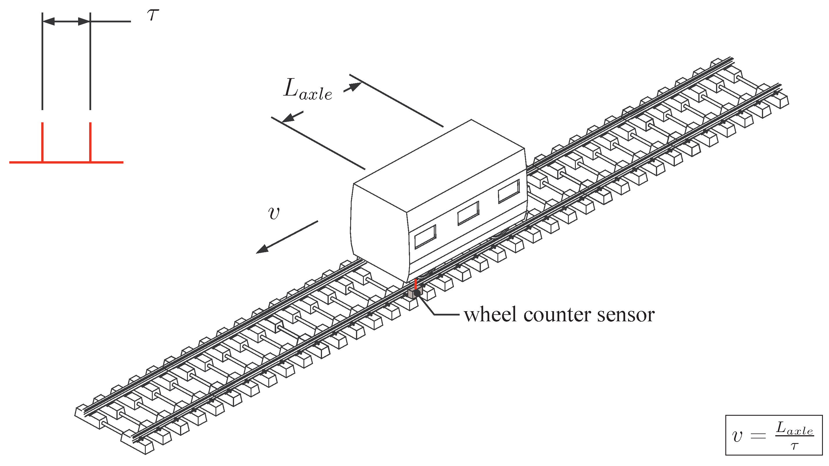
- Kouroussis, G.; Connolly, D.P.; Forde, M.C.; Verlinden, O. Train speed calculation using ground vibrations. J. Rail Rapid Transit 2015, 229, 466–483. [Google Scholar] [CrossRef]
- Paixão, A.; Ribeiro, C.A.; Pinto, N.; Fortunato, E.; Calçada, R. On the use of under sleeper pads in transition zones at railway underpasses: Experimental field testing. Struct. Infrastruct. Eng. 2015, 11, 112–128. [Google Scholar] [CrossRef]
- Liu, C.; Wei, J.; Zhang, Z.; Liang, J.; Ren, T.; Xu, H. Design and evaluation of a remote measurement system for the online monitoring of rail vibration signals. J. Rail Rapid Transit 2014. [Google Scholar] [CrossRef]
- Cañete, E.; Chen, J.; Díaz, M.; Llopis, L.; Rubio, B. Sensor4PRI: A sensor platform for the protection of railway infrastructures. Sensors 2015, 15, 4996–5019. [Google Scholar] [CrossRef] [PubMed]
- Taylor, R. A system for broken rail detection independent of the signalling system. In Proceedings of the IRSE Australasia Technical Meeting, Sydney, Australia, 18 March 2011.
- Caucheteur, C.; Chah, K.; Lhommé, F.; Blondel, M.; Mégret, P. Autocorrelation demodulation technique for fiber Bragg grating sensor. IEEE Photonics Technol. Lett. 2004, 16, 2320–2322. [Google Scholar] [CrossRef]
- Hwang, D.; Seo, D.C.; Kwon, I.B.; Chung, Y. Restoration of reflection spectra in a serial FBG sensor array of a WDM/TDM measurement system. Sensors 2012, 12, 12836–12843. [Google Scholar] [CrossRef]
- Choi, S.J.; Kim, Y.C.; Song, M.; Pan, J.K. A self-referencing intensity-based fiber optic sensor with multipoint sensing characteristics. Sensors 2014, 14, 12803–12815. [Google Scholar] [CrossRef] [PubMed]
- Wei, C.L.; Lai, C.C.; Liu, S.Y.; Chung, W.H.; Ho, T.K.; Tam, H.Y.; Ho, S.L.; McCusker, A.; Kam, J.; Lee, K.Y. A fiber Bragg grating sensor system for train axle counting. IEEE Sens. J. 2010, 10, 1905–1912. [Google Scholar]
- Filograno, M.L.; Corredera, P.; Rodriguez-Barrios, A.; Martin-Lopez, S.; Rodriguez-Plaza, M.; Andres-Alguacil, A.; Gonzalez-Herraez, M. Real time monitoring of railway traffic using fiber Bragg grating sensors. IEEE Sens. J. 2010, 12, 85–92. [Google Scholar] [CrossRef]
- Mennella, F.; Laudati, A.; Esposito, M.; Cusano, A.; Cutolo, A.; Giordano, M.; Campopiano, S.; Bregliot, G. Railway monitoring and train tracking by fiber Bragg grating sensors. Proc. SPIE 2007, 6619. [Google Scholar] [CrossRef]
- Filograno, M.L.; Corredera, P.; Gonzalez-Herraez, M.; Rodriguez-Plaza, M.; Andres-Alguacil, A. Wheel flat detection in high-speed railway systems using fiber Bragg gratings. IEEE Sens. J. 2013, 13, 4808–4816. [Google Scholar] [CrossRef]
- Kluth, R.; Watley, D.; Farhadiroushan, M.; Park, D.S.; Lee, S.U.; Kim, J.Y.; Kim, Y.S. Case studies on distributed temperature and strain sensing (DTSS) by using optic fibre. In Proceedings of the International Conference on Condition Monitoring and Diagnosis, Changwon, Korea, 2–5 April 2006.
- Yoon, H.J.; Song, K.Y.; Kim, J.S.; Kim, D.S. Longitudinal strain monitoring of rail using a distributed fiber sensor based on Brillouin optical correlation domain analysis. NDT&E Int. 2011, 44, 637–644. [Google Scholar] [CrossRef]
- Minardo, A.; Porcaro, G.; Giannetta, D.; Bernini, R.; Zeni, L. Real-time monitoring of railway traffic using slope-assisted Brillouin distributed sensors. Appl. Opt. 2013, 52, 3770–3776. [Google Scholar] [CrossRef] [PubMed]
- Kerrouche, A.; Boyle, W.J.O.; Gebremichael, Y.; Sun, T.; Grattan, K.T.V.; Täljsten, B.; Bennitz, A. Field tests of fibre Bragg grating sensors incorporated into CFRP for railway bridge strengthening condition monitoring. Sens. Actuators A Phys. 2008, 148, 68–74. [Google Scholar] [CrossRef]
- Laffont, G.; Roussel, N.; Rougeault, S.; Boussoir, J.; Maurin, L.; Ferdinand, P. Innovative FBG sensing techniques for the railway industry: application to overhead contact line monitoring. Proc. SPIE 2009, 7503. [Google Scholar] [CrossRef]
- Shatalin, S.; Treschikov, V.N.; Rogers, A.J. Interferometric optical time-domain reflectometry for distributed optical-fiber sensing. Appl. Opt. 1998, 37, 5600–5604. [Google Scholar] [CrossRef] [PubMed]
- Fotech Solutions. Available online: http://www.fotechsolutions.com/ (accessed on 28 June 2015).
- Kessell, C. Acoustic sensing: The future for rail monitoring? Rail Eng. 2014, 114, 32–34. [Google Scholar]
- International Electrotechnical Commission. IEC 61508: Functional Safety of Electrical/Electronic/Programmable Electronic Safety-Related Systems—Part 1: General Requirements; International Electrotechnical Commission: Geneva, Switzerland, 2010. [Google Scholar]
- International Electrotechnical Commission. IEC 62279: Railway Applications—Communications, Signalling and Processing Systems—Software for Railway Control and Protection Systems; International Electrotechnical Commission: Geneva, Switzerland, 2002. [Google Scholar]
© 2015 by the authors; licensee MDPI, Basel, Switzerland. This article is an open access article distributed under the terms and conditions of the Creative Commons Attribution license (http://creativecommons.org/licenses/by/4.0/).
Share and Cite
Kouroussis, G.; Caucheteur, C.; Kinet, D.; Alexandrou, G.; Verlinden, O.; Moeyaert, V. Review of Trackside Monitoring Solutions: From Strain Gages to Optical Fibre Sensors. Sensors 2015, 15, 20115-20139. https://doi.org/10.3390/s150820115
Kouroussis G, Caucheteur C, Kinet D, Alexandrou G, Verlinden O, Moeyaert V. Review of Trackside Monitoring Solutions: From Strain Gages to Optical Fibre Sensors. Sensors. 2015; 15(8):20115-20139. https://doi.org/10.3390/s150820115
Chicago/Turabian StyleKouroussis, Georges, Christophe Caucheteur, Damien Kinet, Georgios Alexandrou, Olivier Verlinden, and Véronique Moeyaert. 2015. "Review of Trackside Monitoring Solutions: From Strain Gages to Optical Fibre Sensors" Sensors 15, no. 8: 20115-20139. https://doi.org/10.3390/s150820115