
Simultaneous Localization and Mapping with Iterative Sparse Extended Information Filter for Autonomous Vehicles


Abstract
:1. Introduction
2. The Iterative SEIF
2.1. Review of SEIF
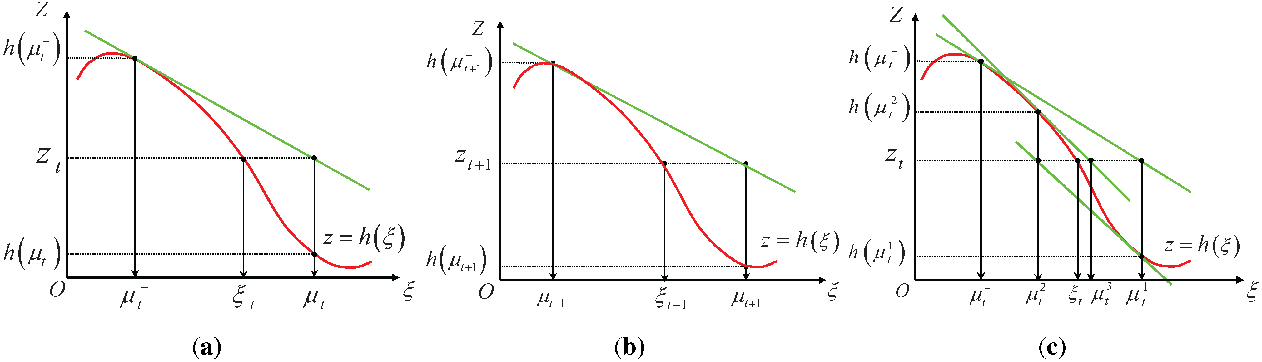
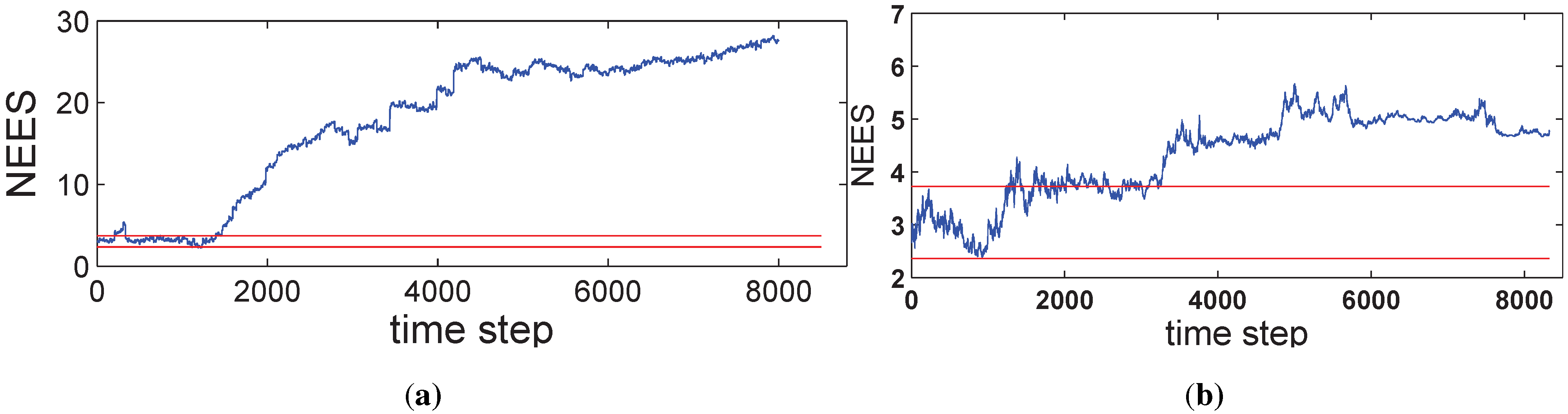
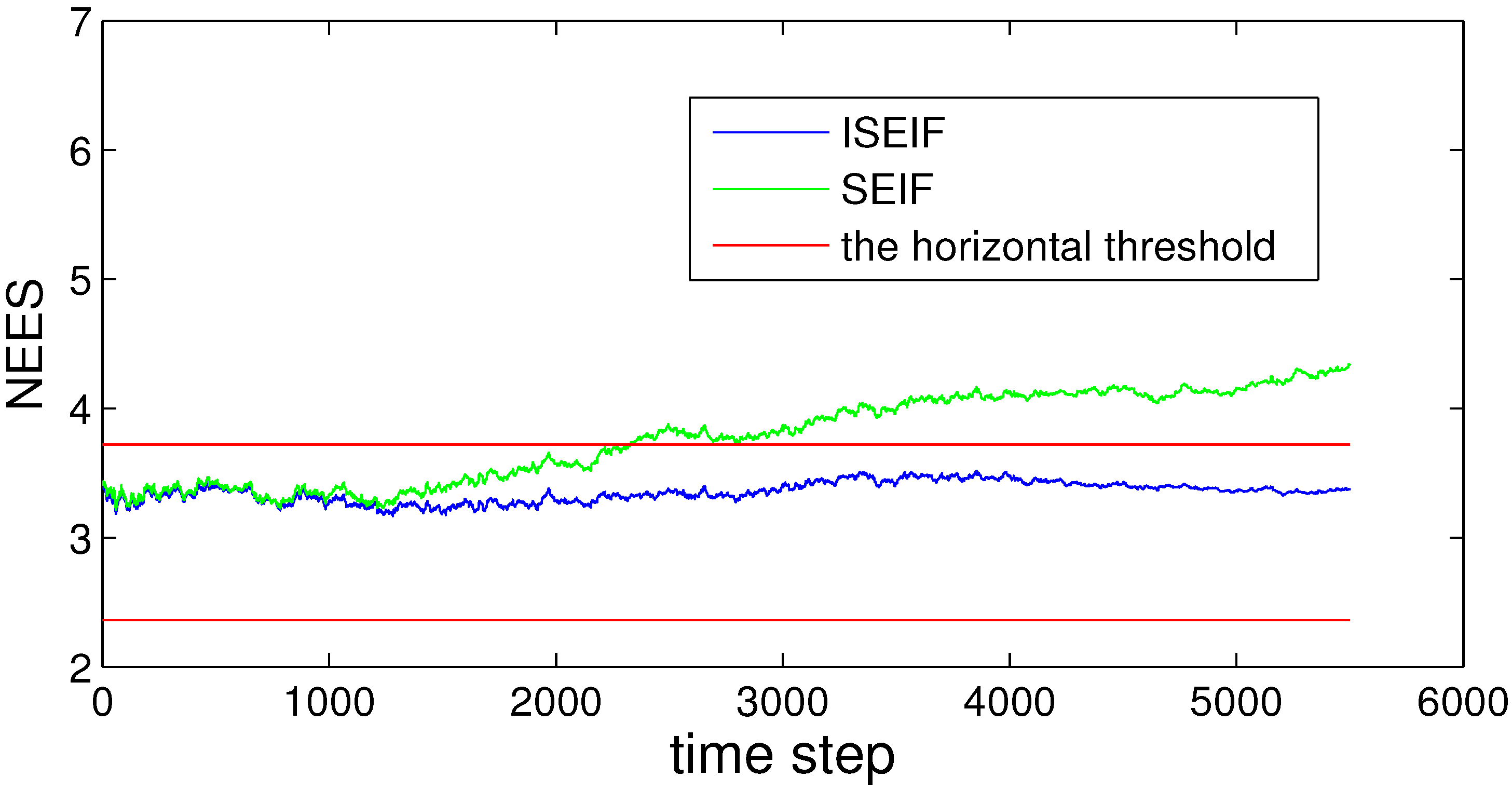
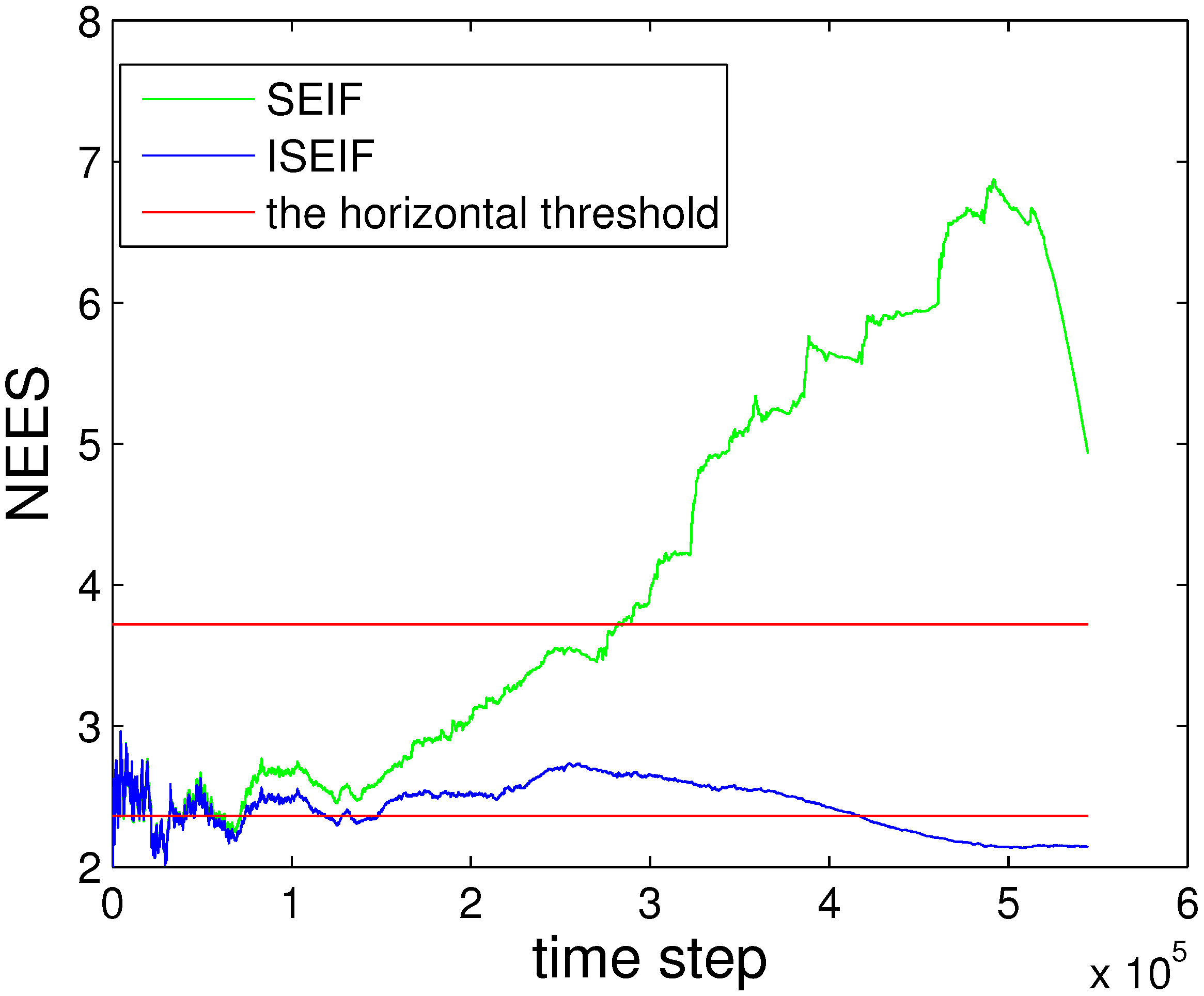
2.2. Consistency Analysis of SEIF

2.3. The Adaptive ISEIF
- The nonlinear motion and measurement model functions are given as follows:
- Initialization as follows:
- For , do the following:
- (a)
- Perform motion update equations of SEIF. The iterative SEIF is the same as the SEIF up to this point.
- (b)
- If t is not in the iterative periods, skip to d; else start to perform iterative steps as follows: Initialize the iterative SEIF to the standard SEIF and perform the iterative measurement update step.Calculate the measurement update Equations (14) to (18).
- (c)
- Calculate the value of delta:According to the adaptive stop criteria, if is smaller than the threshold, stop the iteration process and turn to d; otherwise, return to the b step to continue the iteration.
- (d)
- The final information matrix and information vector are given as follows:where n is the number of iterations.
- Perform the sparsification step of SEIF.
3. Experiments
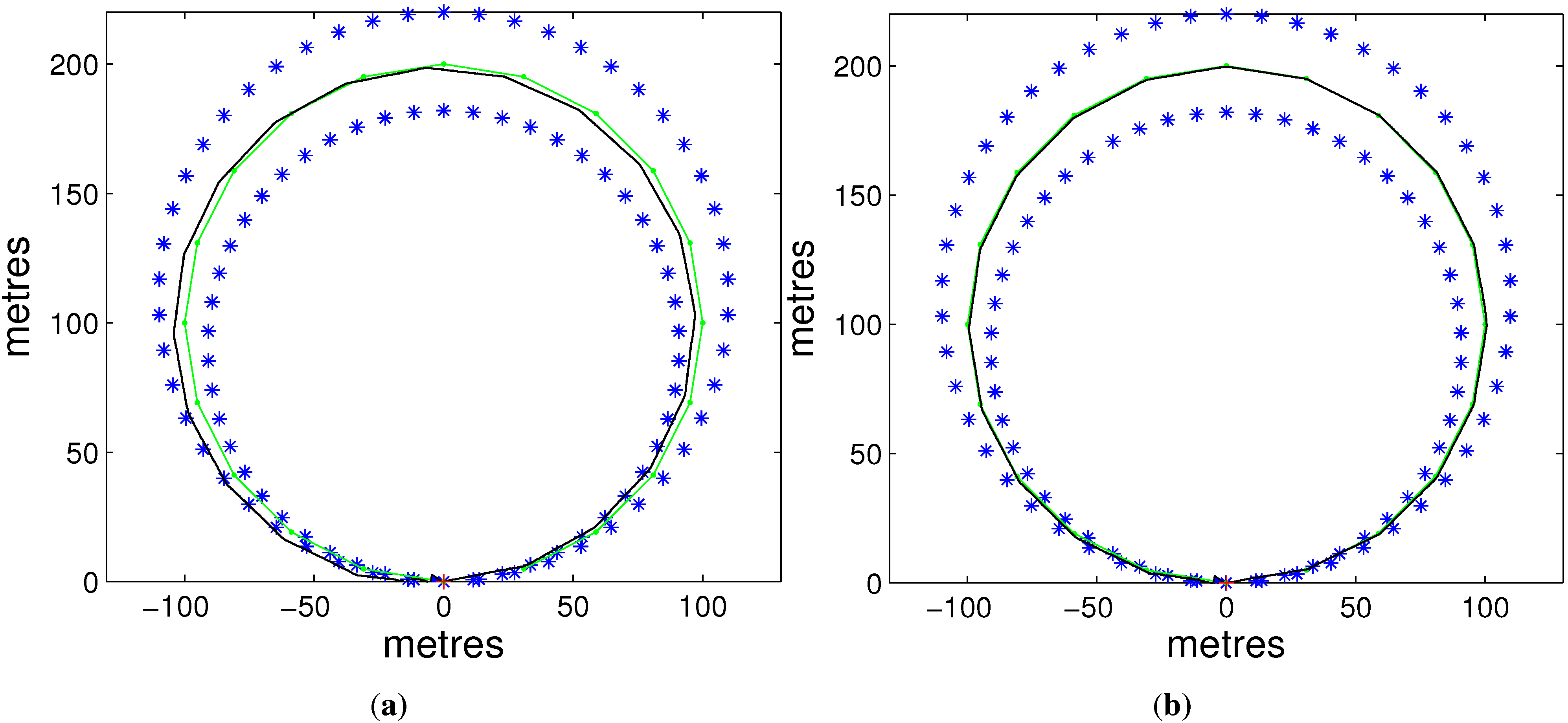
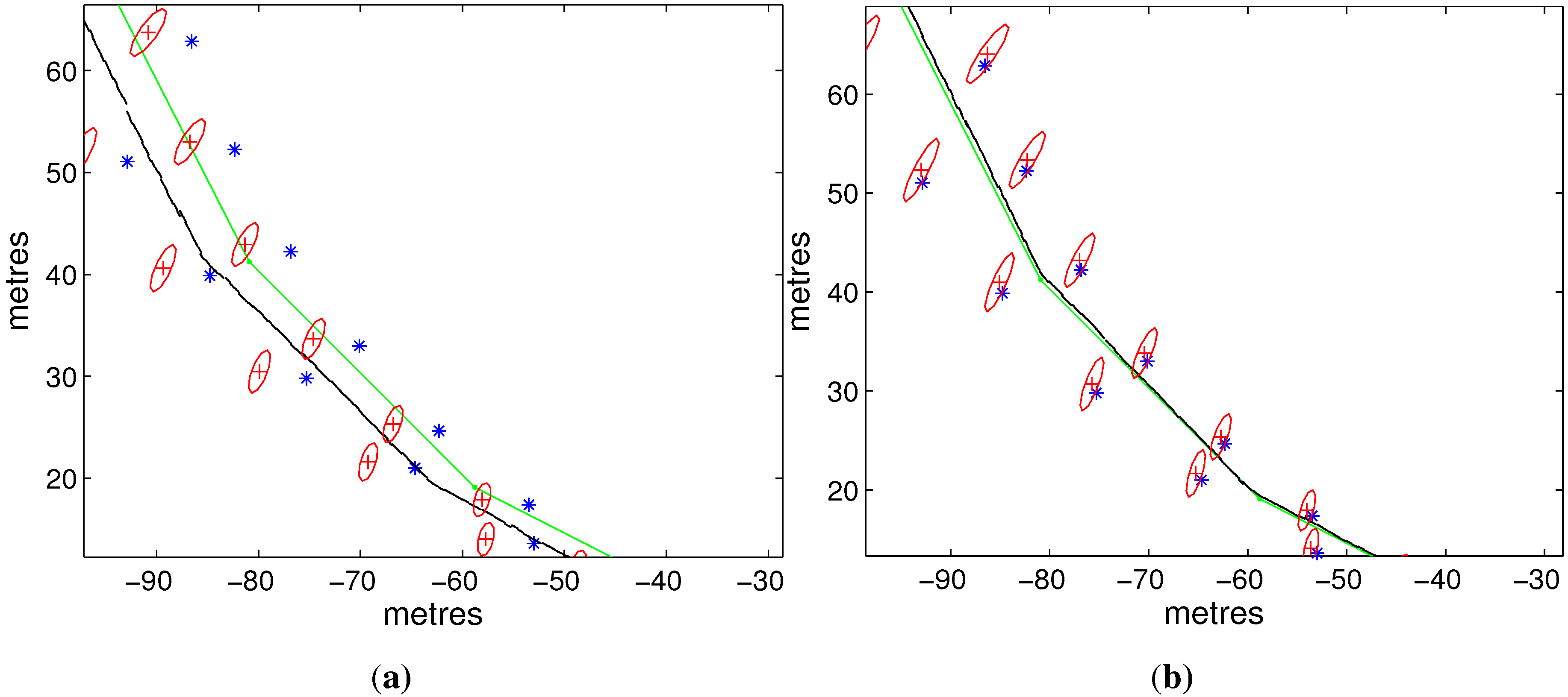
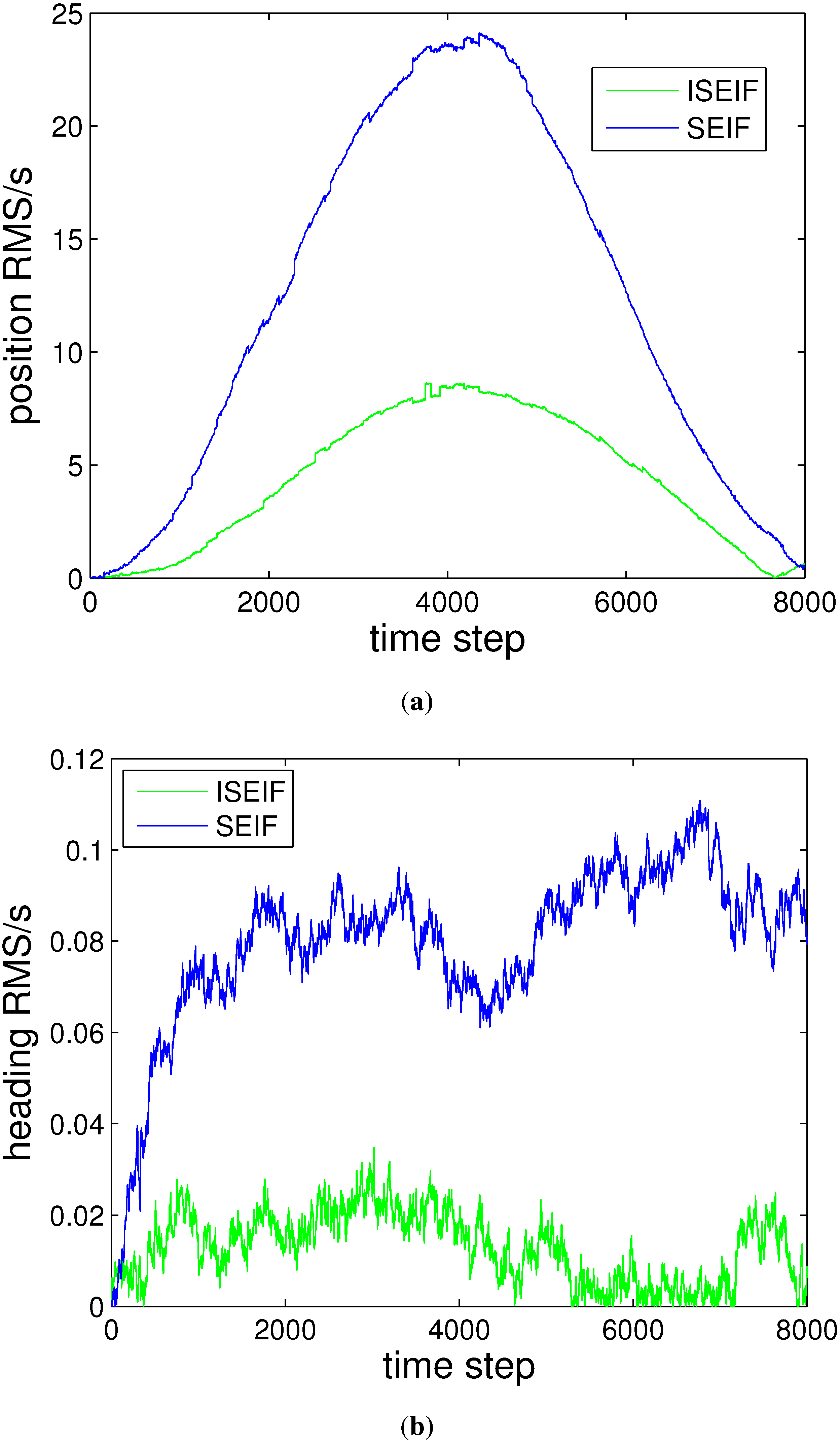
3.1. Simulations

| Wheelbase of vehicle | 4 m | Control noise | (0.3 m/s, ) |
| Speed | 3 m/s | Observation noise | (0.2 m/s, ) |
| Maximum steering angle | Control frequency | 40 Hz | |
| Maximum range | 30 m | Observation frequency | 5 Hz |


| Pose-x Error | Pose-y Error | Heading Error | Landmark-x Error | Landmark-y Error | |
|---|---|---|---|---|---|
| SEIF | 19.9203 m | 9.1883 m | 18.9011 m | 9.9527 m | |
| ISEIF | 15.8803 m | 7.6626 m | 14.1157 m | 7.6663 m |

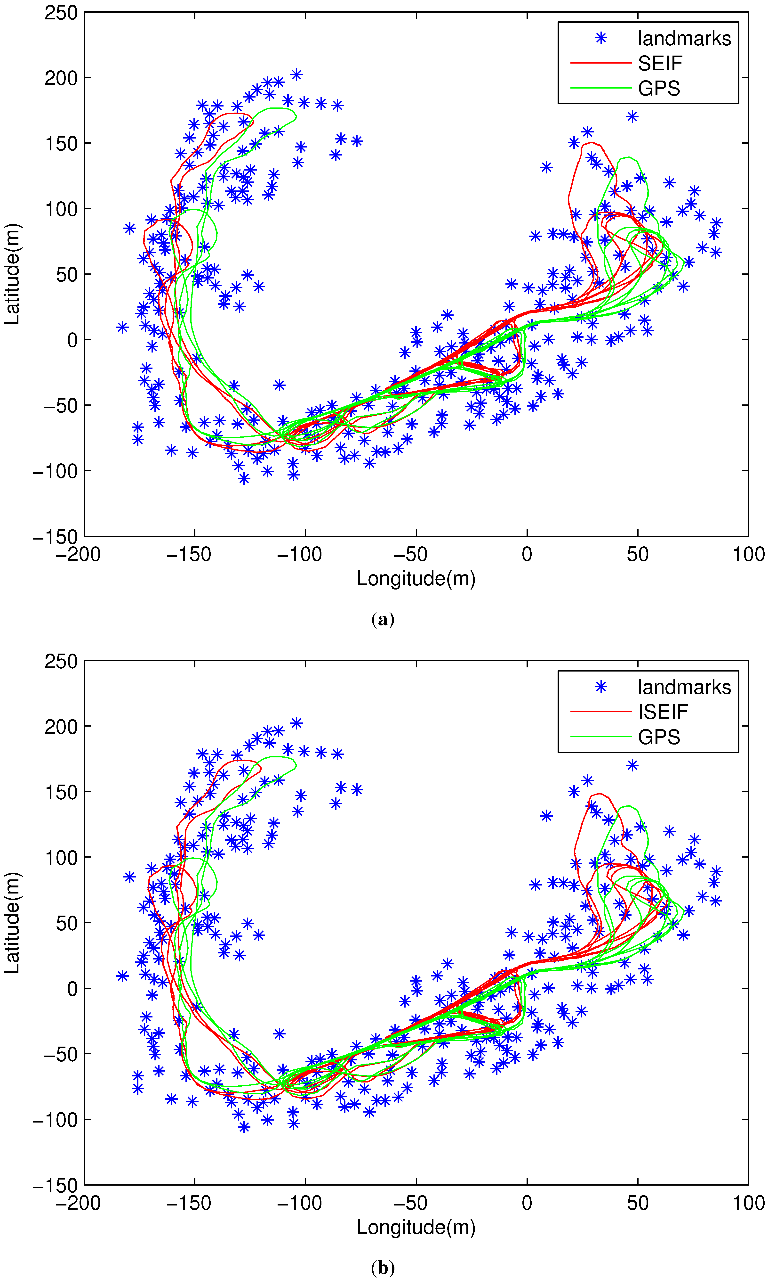
3.2. Victoria Park Dataset
3.2.1. Sensors
3.2.2. Results


| Algorithm | Pose-x Error | Pose-y Error | NEES | CPU Elapsed Time |
|---|---|---|---|---|
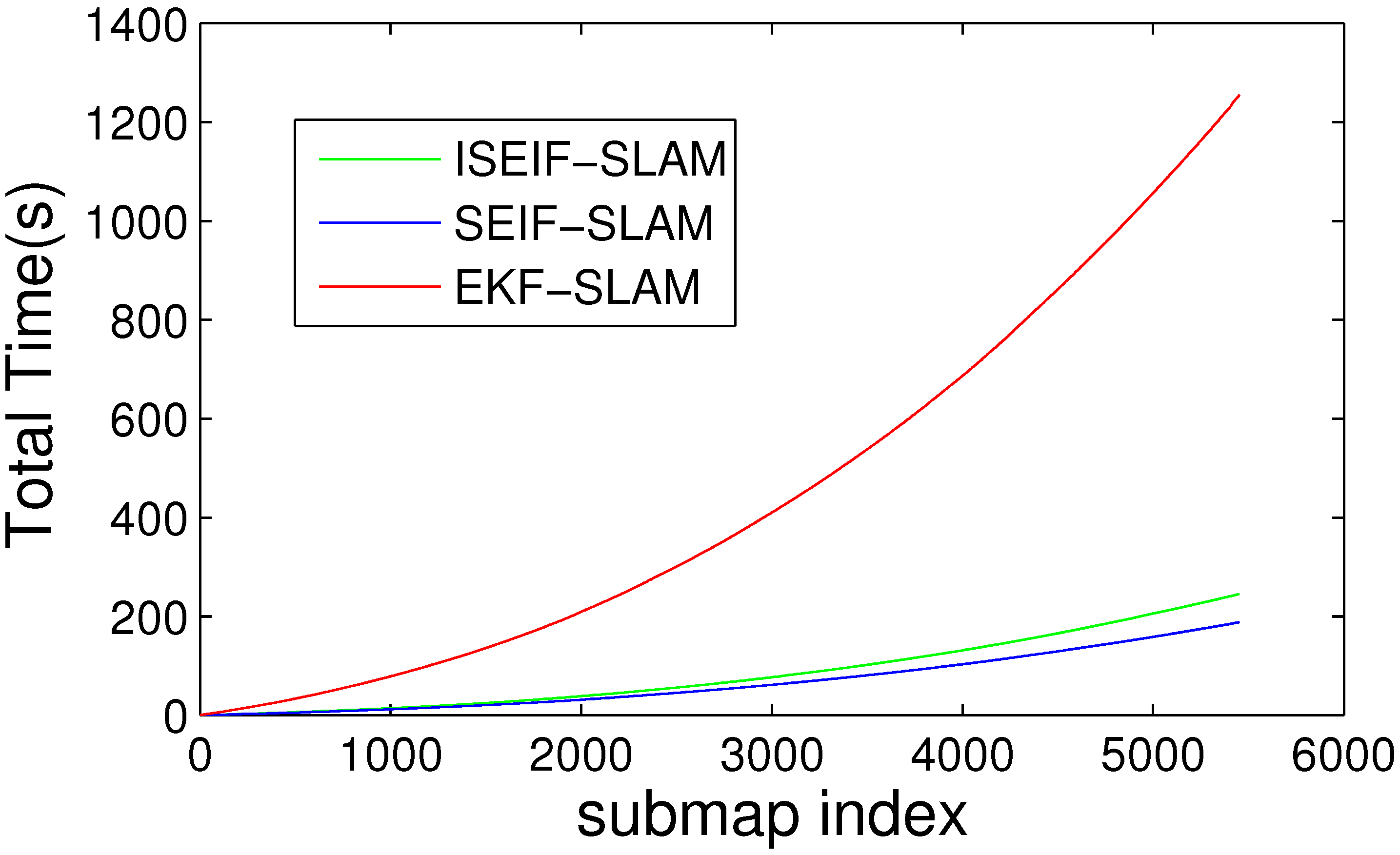
| SEIF | 7.5284 m | 5.3781 m | 51.10% | 1374.28 s |
| ISEIF | 4.7133 m | 4.8325 m | 82.34% | 1658.31 s |
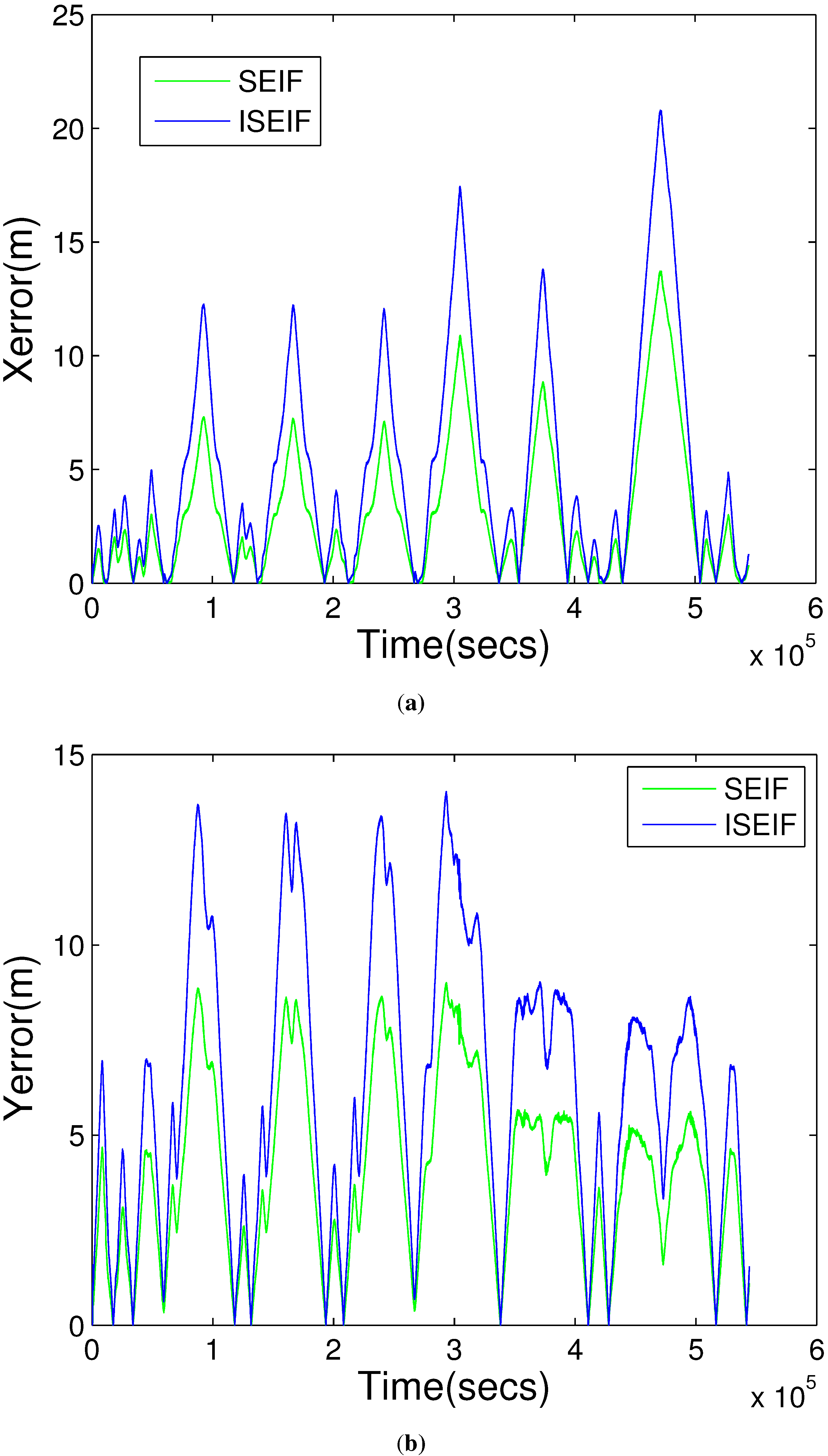
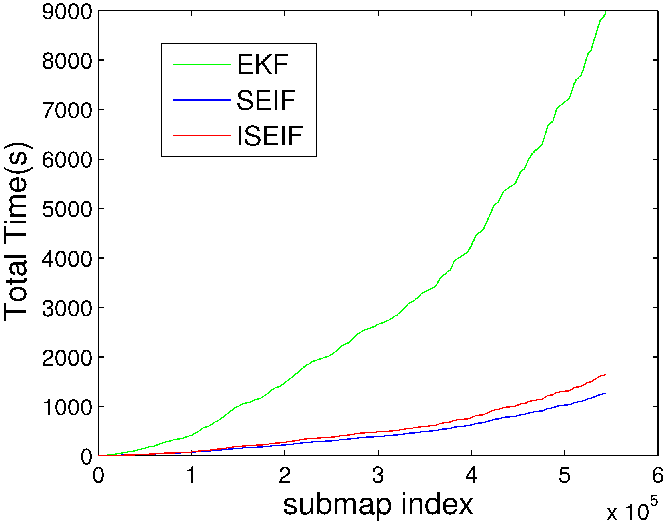
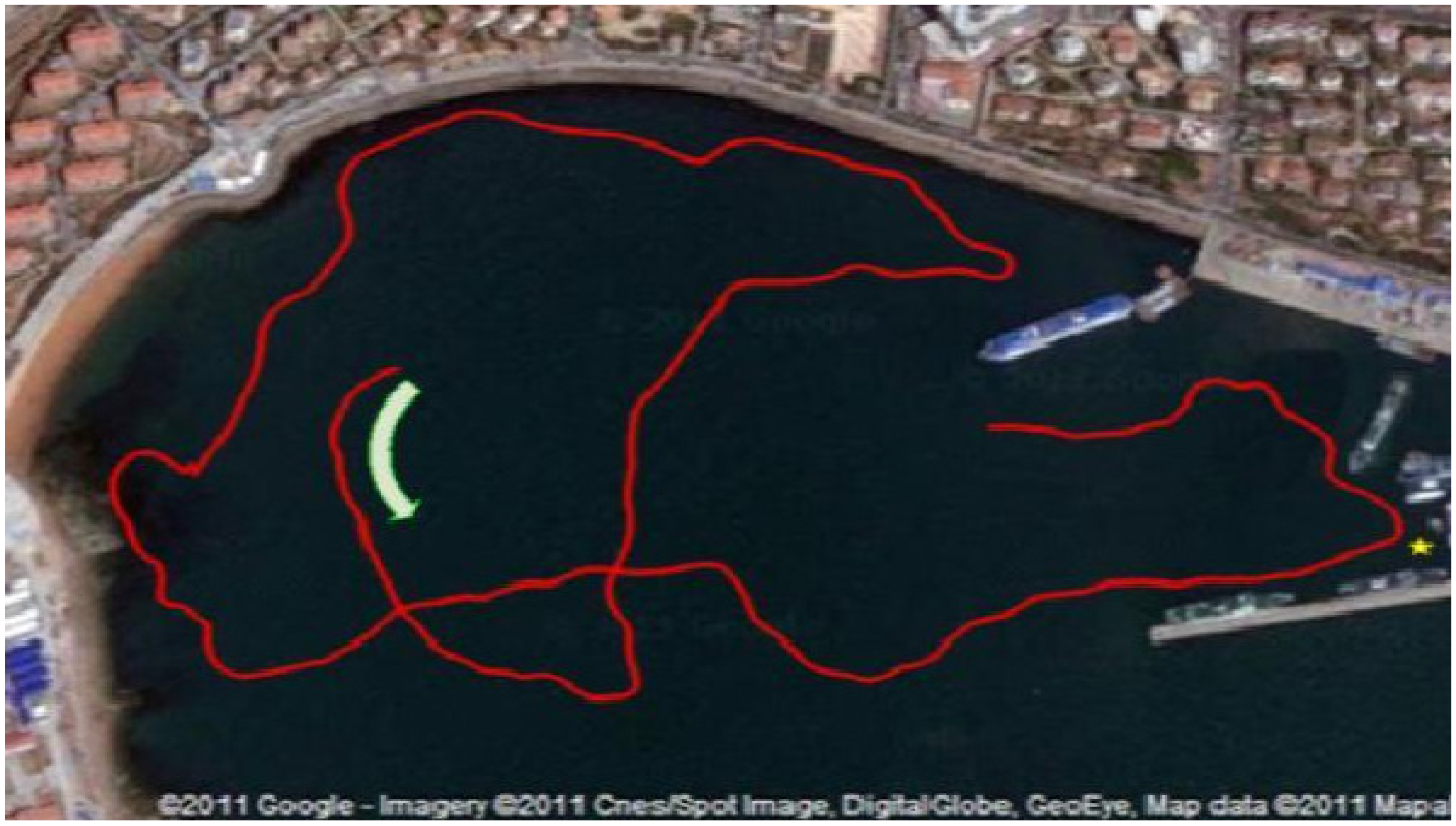
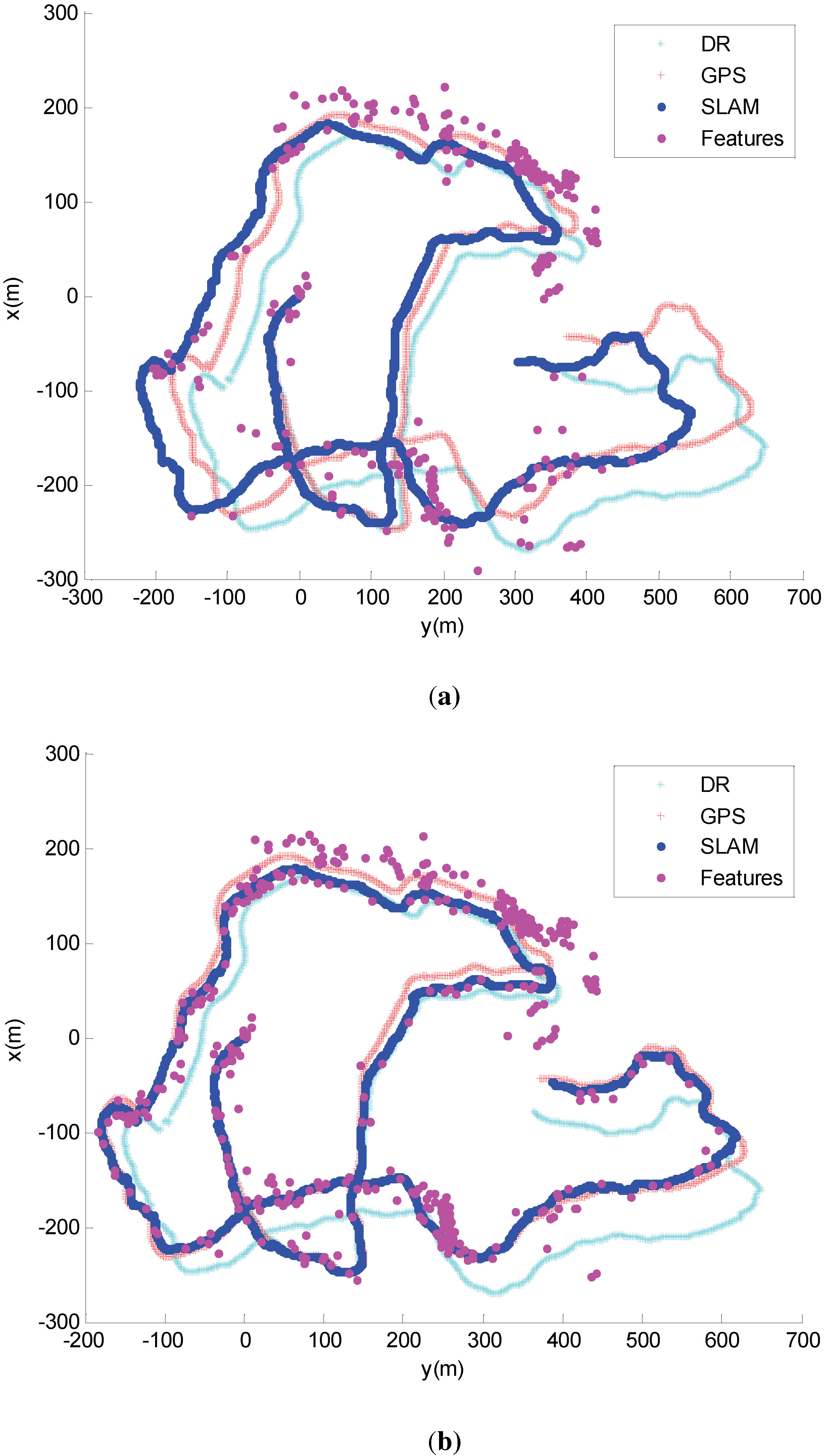
3.3. Sea Trials in Tuandao Bay
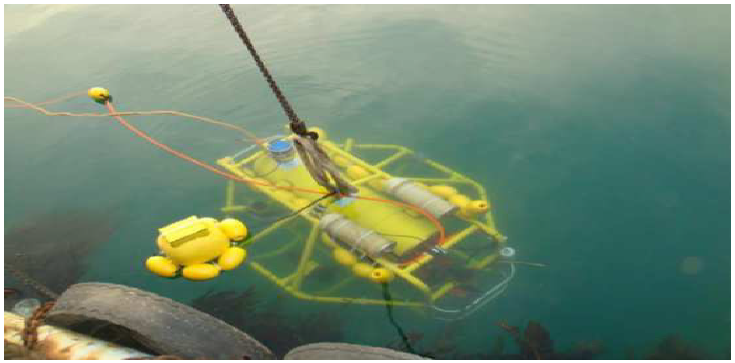
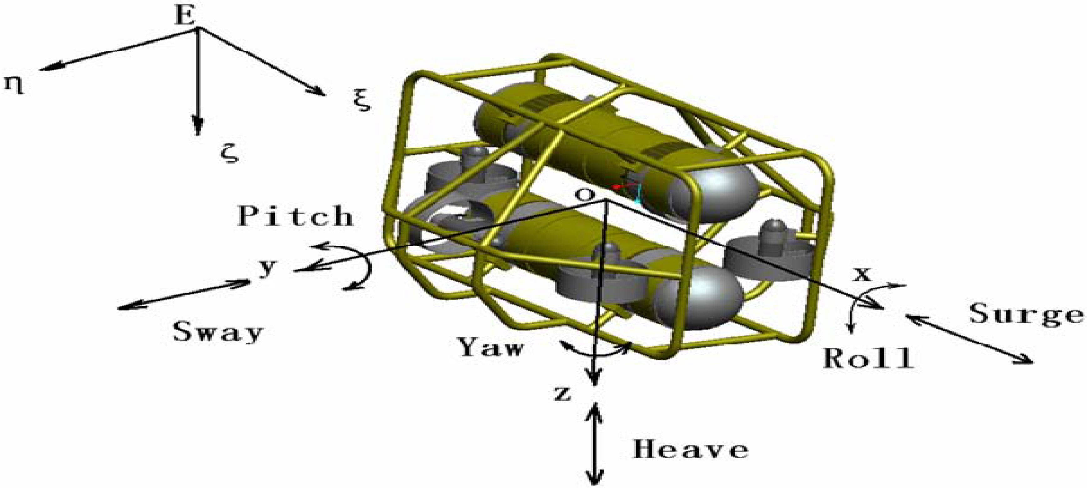
3.3.1. AUV C-Ranger

| Parameter | Length | Width | Height | Tonnage | Weight | Maximal Speed | Endurance |
|---|---|---|---|---|---|---|---|
| Value | 1.6 m | 1.3 m | 1.1 m | 208 L | 206 kg (full loaded) | 3 knots (1.5 m/s) | 8 h at 1 knot speed |
3.3.2. On-Board Sensors
3.3.3. AUV Motion Model
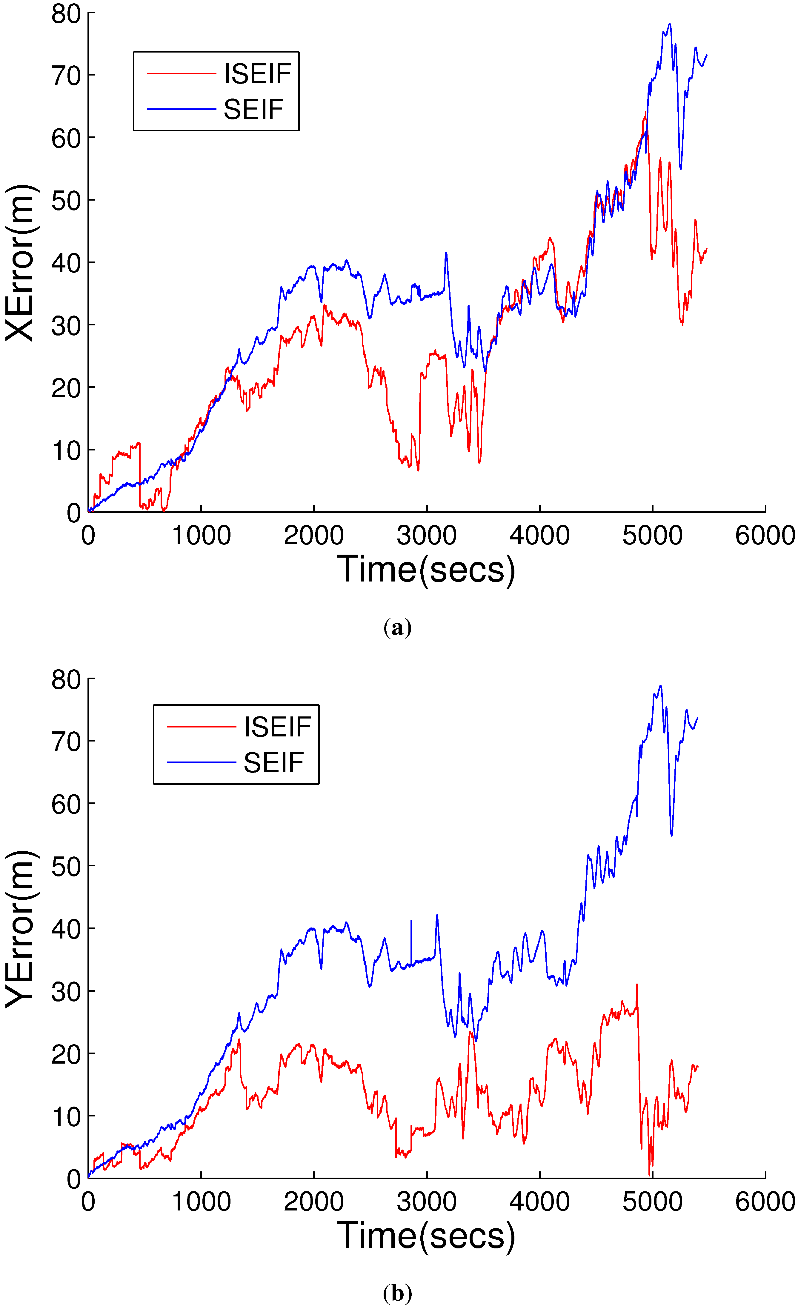
3.3.4. Sea Trial


| Algorithm | Pose-x Error | Pose-y Error | NEES | CPU Elapsed Time |
|---|---|---|---|---|
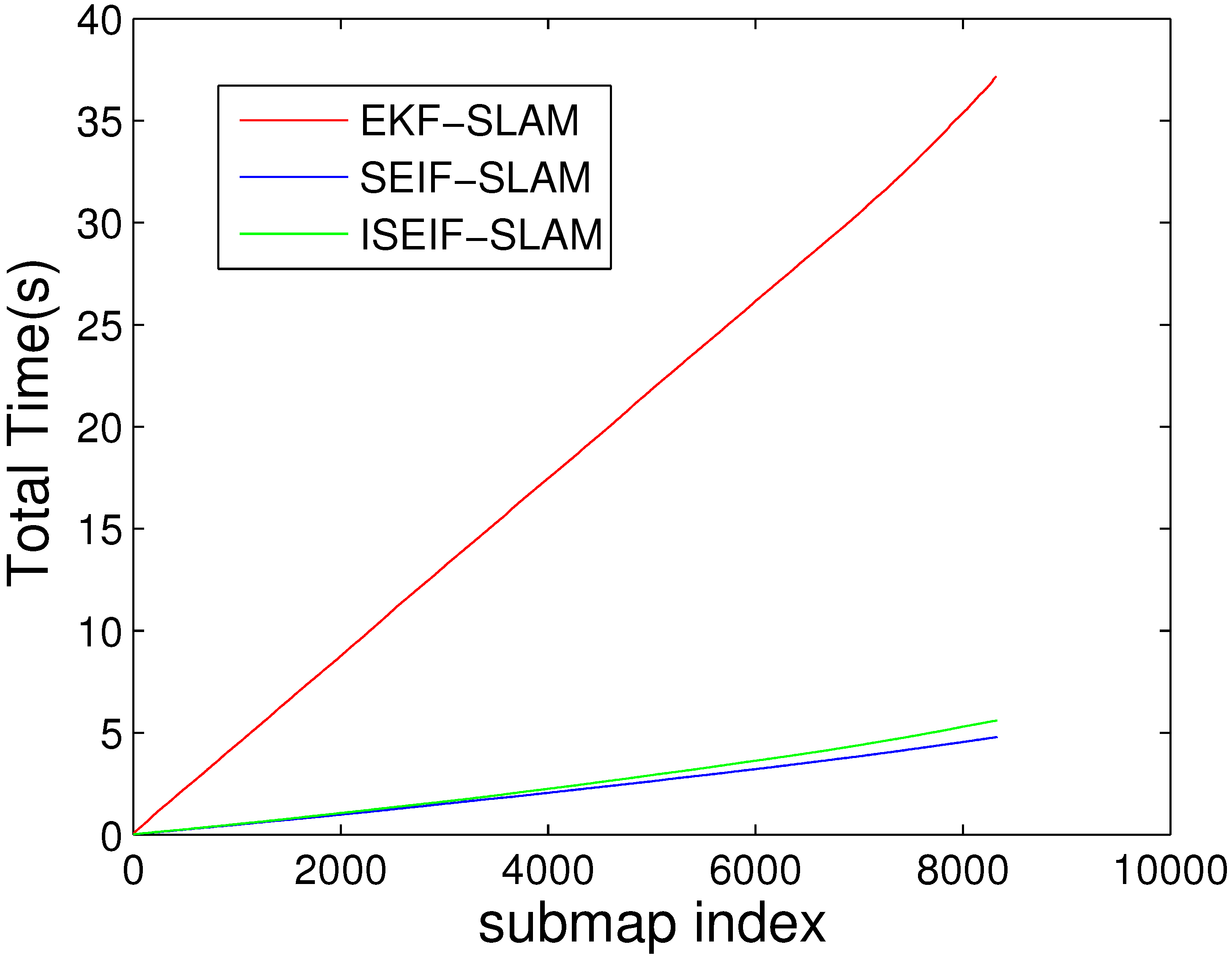
| SEIF | 36.4628 m | 40.7963 m | 48.23% | 285.23 s |
| ISEIF | 27.7952 m | 12.1165 m | 100% | 199.58 s |
4. Discussion
5. Conclusions
Acknowledgments
Author Contributions
Conflicts of Interest
References
- Paull, L.; Saeedi, S.; Seto, M.; Li, H. AUV Navigation and Localization: A Review. IEEE J. Ocean. Eng. 2014, 39, 131–149. [Google Scholar] [CrossRef]
- Kharchenko, V.; Kondratyuk, V.; Ilnytska, S.; Kutsenko, O.; Larin, V. Urgent problems of UAV navigation system development and practical implementation. In Proceedings of the 2013 IEEE 2nd International Conference on Actual Problems of Unmanned Air Vehicles Developments Proceedings (APUAVD), Kiev, Ukraine, 15–17 October 2013; pp. 157–160.
- Li, Q.; Chen, L.; Li, M.; Shaw, S.L.; Nuchter, A. A Sensor-Fusion Drivable-Region and Lane-Detection System for Autonomous Vehicle Navigation in Challenging Road Scenarios. IEEE Trans. Veh. Technol. 2014, 63, 540–555. [Google Scholar] [CrossRef]
- Smith, R.; Self, M.; Cheeseman, P. Estimating Uncertain Spatial Relationships in Robotics. In Autonomous Robot Vehicles; Springer-Verlag New York, Inc.: New York, NY, USA, 1990; pp. 167–193. [Google Scholar]
- Matsebe, O. EKF-SLAM Based Navigation System for an AUV; CSIR: Pretoria, South Africa, 2008. [Google Scholar]
- Vazquez-Martin, R.; Nuñez, P.; del Toro, J.; Bandera, A.; Sandoval, F. Adaptive observation covariance for EKF-SLAM in indoor environments using laser data. In Proceedings of the Electrotechnical Conference 2006 (MELECON 2006), Malaga, Spain, 16–19 May 2006; pp. 445–448.
- Thrun, S.; Burgard, W.; Fox, D. Probabilistic Robotics; MIT Press: Cambridge, MA, USA, 2005. [Google Scholar]
- Maybeck, P.S. Stochastic Models, Estimation, and Control; Academic Press: Waltham, MA, USA, 1982; Volume 3. [Google Scholar]
- Thrun, S.; Liu, Y.; Koller, D.; Ng, A.Y.; Ghahramani, Z.; Durrant-Whyte, H. Simultaneous localization and mapping with sparse extended information filters. Int. J. Robot. Res. 2004, 23, 693–716. [Google Scholar] [CrossRef]
- Frese, U.; Hirzinger, G. Simultaneous localization and mapping—A discussion. In Proceedings of the IJCAI Workshop on Reasoning with Uncertainty in Robotics, Seattle, WA, USA, 4–10 August 2001; pp. 17–26.
- Durrant-Whyte, H.; Bailey, T. Simultaneous localization and mapping: Part I. IEEE Robot. Autom. Mag. 2006, 13, 99–110. [Google Scholar] [CrossRef]
- Bailey, T.; Durrant-Whyte, H. Simultaneous localization and mapping (SLAM): Part II. IEEE Robot. Autom. Mag. 2006, 13, 108–117. [Google Scholar] [CrossRef]
- Montemerlo, M.; Thrun, S.; Koller, D.; Wegbreit, B. FastSLAM: A Factored Solution to the Simultaneous Localization and Mapping Problem; AAAI/IAAI: Edmonton, AB, Canada, 2002; pp. 593–598. [Google Scholar]
- Montemerlo, M.; Thrun, S. FastSLAM 2.0. In FastSLAM: A Scalable Method for the Simultaneous Localization and Mapping Problem in Robotics; Springer: Berlin/Heidelberg, Germany, 2007; pp. 63–90. [Google Scholar]
- Bailey, T.; Nieto, J.; Guivant, J.; Stevens, M.; Nebot, E. Consistency of the EKF-SLAM algorithm. In Proceedings of the 2006 IEEE/RSJ International Conference on Intelligent Robots and Systems, Beijing, China, 9–15 October 2006; IEEE, 2006; pp. 3562–3568. [Google Scholar]
- Liu, Y.; Thrun, S. Results for Outdoor-SLAM Using Sparse Extended Information Filters; ICRA: Gurgaon, India, 2003; pp. 1227–1233. [Google Scholar]
- Thrun, S.; Liu, Y. Multi-robot SLAM with sparse extended information filers. In Robotics Research; Springer: Berlin/Heidelberg, Germany, 2005; pp. 254–266. [Google Scholar]
- Eustice, R.; Walter, M.; Leonard, J. Sparse extended information filters: Insights into sparsification. In Proceedings of the 2005 IEEE/RSJ International Conference on Intelligent Robots and Systems 2005 (IROS 2005), Edmonton, AB, Canada, 2–6 August 2005; pp. 3281–3288.
- Walter, M.R.; Eustice, R.M.; Leonard, J.J. Exactly sparse extended information filters for feature-based SLAM. Int. J. Robot. Res. 2007, 26, 335–359. [Google Scholar] [CrossRef]
- Walter, M.; Hover, F.; Leonard, J. SLAM for ship hull inspection using exactly sparse extended information filters. In Proceedings of the IEEE International Conference on Robotics and Automation (ICRA 2008), Pasadena, CA, USA, 19–23 May 2008; pp. 1463–1470.
- Gutmann, J.S.; Eade, E.; Fong, P.; Munich, M.E. A Constant-Time Algorithm for Vector Field SLAM using an Exactly Sparse Extended Information Filter. In Robotics: Science and Systems; The MIT Press: Cambridge, MA, USA, 2010. [Google Scholar]
- Eustice, R.M.; Singh, H.; Leonard, J.J. Exactly sparse delayed-state filters. In Proceedings of the 2005 IEEE International Conference on Robotics and Automation (ICRA 2005), Barcelona, Spain, 18–22 April 2005; pp. 2417–2424.
- Simon, D. Optimal State Estimation: Kalman, H infinity, and Nonlinear Approaches; John Wiley & Sons: Hoboken, NJ, USA, 2006. [Google Scholar]
- Shojaei, K.; Shahri, A.M. Experimental study of iterated Kalman filters for simultaneous localization and mapping of autonomous mobile robots. J. Intell. Robot. Syst. 2011, 63, 575–594. [Google Scholar] [CrossRef]
- Zhou, W.; Zhao, C.; Guo, J. The study of improving Kalman filters family for nonlinear SLAM. J. Intell. Robot. Syst. 2009, 56, 543–564. [Google Scholar] [CrossRef]
- Lefebvre, T.; Bruyninckx, H.; De Schutter, J. Kalman filters for non-linear systems: A comparison of performance. Int. J. Control 2004, 77, 639–653. [Google Scholar] [CrossRef]
- Guivant, J. Victoria Park. Available online: http://www-personal.acfr.usyd.edu.au/nebot/victoria_park.htm (accessed on 15 December 2013).
- He, B.; Wang, B.; Yan, T.; Han, Y. A Distributed Parallel Motion Control for the Multi-Thruster Autonomous Underwater Vehicle. Mech. Based Des. Struct. Mach. 2013, 41, 236–257. [Google Scholar] [CrossRef]
- He, B.; Liang, Y.; Feng, X.; Nian, R.; Yan, T.; Li, M.; Zhang, S. AUV SLAM and experiments using a mechanical scanning forward-looking sonar. Sensors 2012, 12, 9386–9410. [Google Scholar] [CrossRef] [PubMed] [Green Version]
- Subudhi, B.; Mukherjee, K.; Ghosh, S. A static output feedback control design for path following of autonomous underwater vehicle in vertical plane. Ocean Eng. 2013, 63, 72–76. [Google Scholar] [CrossRef]
- Kuwata, Y.; Wolf, M.T.; Zarzhitsky, D.; Huntsberger, T.L. Safe Maritime Autonomous Navigation with COLREGS, Using Velocity Obstacles. IEEE J. Ocean. Eng. 39, 110–119. [CrossRef]
- Bar-Shalom, Y.; Li, X.R.; Kirubarajan, T. Estimation with Applications to Tracking and Navigation: Theory Algorithms and Software; John Wiley & Sons: Hoboken, NJ, USA, 2004. [Google Scholar]
- Guivant, J.E.; Nebot, E.M. Solving computational and memory requirements of feature-based simultaneous localization and mapping algorithms. IEEE Trans. Robot. Autom. 2003, 19, 749–755. [Google Scholar] [CrossRef]
- Huang, G.; Mourikis, A.; Roumeliotis, S. A Quadratic-Complexity Observability-Constrained Unscented Kalman Filter for SLAM. IEEE Trans. Robot. 2013, 29, 1226–1243. [Google Scholar] [CrossRef]
- Hesch, J.; Kottas, D.; Bowman, S.; Roumeliotis, S. Consistency Analysis and Improvement of Vision-aided Inertial Navigation. IEEE Trans. Robot. 2014, 30, 158–176. [Google Scholar] [CrossRef]
- Kim, A.; Eustice, R. Real-Time Visual SLAM for Autonomous Underwater Hull Inspection Using Visual Saliency. IEEE Trans. Robot. 2013, 29, 719–733. [Google Scholar] [CrossRef]
- Dellaert, F.; Kaess, M. Square Root SAM: Simultaneous localization and mapping via square root information smoothing. Int. J. Robot. Res. 2006, 25, 1181–1203. [Google Scholar] [CrossRef]
- Kummerle, R.; Grisetti, G.; Strasdat, H.; Konolige, K.; Burgard, W. g2o: A general framework for graph optimization. In Proceedings of the 2011 IEEE International Conference on Robotics and Automation (ICRA), Shanghai, China, 9–13 May 2011; pp. 3607–3613.
- Sunderhauf, N.; Protzel, P. Switchable constraints vs. max-mixture models vs. RRR—A comparison of three approaches to robust pose graph SLAM. In Proceedings of the 2013 IEEE International Conference on Robotics and Automation (ICRA), Karlsruhe, Germany, 6–10 May 2013; pp. 5198–5203.
- Fallon, M.; Folkesson, J.; McClelland, H.; Leonard, J. Relocating Underwater Features Autonomously Using Sonar-Based SLAM. IEEE J. Ocean. Eng. 2013, 38, 500–513. [Google Scholar] [CrossRef]
- Lee, S.; Lee, S. Embedded Visual SLAM: Applications for Low-Cost Consumer Robots. IEEE Robot. Autom. Mag. 2013, 20, 83–95. [Google Scholar] [CrossRef]
- Lategahn, H.; Stiller, C. Vision-Only Localization. IEEE Trans. Intell. Transp. Syst. 2014, 15, 1246–1257. [Google Scholar] [CrossRef]
© 2015 by the authors; licensee MDPI, Basel, Switzerland. This article is an open access article distributed under the terms and conditions of the Creative Commons Attribution license (http://creativecommons.org/licenses/by/4.0/).
Share and Cite
He, B.; Liu, Y.; Dong, D.; Shen, Y.; Yan, T.; Nian, R. Simultaneous Localization and Mapping with Iterative Sparse Extended Information Filter for Autonomous Vehicles. Sensors 2015, 15, 19852-19879. https://doi.org/10.3390/s150819852
He B, Liu Y, Dong D, Shen Y, Yan T, Nian R. Simultaneous Localization and Mapping with Iterative Sparse Extended Information Filter for Autonomous Vehicles. Sensors. 2015; 15(8):19852-19879. https://doi.org/10.3390/s150819852
Chicago/Turabian StyleHe, Bo, Yang Liu, Diya Dong, Yue Shen, Tianhong Yan, and Rui Nian. 2015. "Simultaneous Localization and Mapping with Iterative Sparse Extended Information Filter for Autonomous Vehicles" Sensors 15, no. 8: 19852-19879. https://doi.org/10.3390/s150819852