5.1. Simulation Setup
The proposed model was evaluated using a two-hour excerpt of the TAPASCologne vehicular mobility trace generated for the city of Cologne, Germany [
24]. TAPASCologne is an initiative by the Institute of Transportation Systems at the German Aerospace Center (ITS-DLR), aimed at reproducing realistic car traffic in the greater urban area of the city of Cologne in Germany. Vehicle mobility was generated synthetically using the SUMO microscopic vehicular mobility simulator [
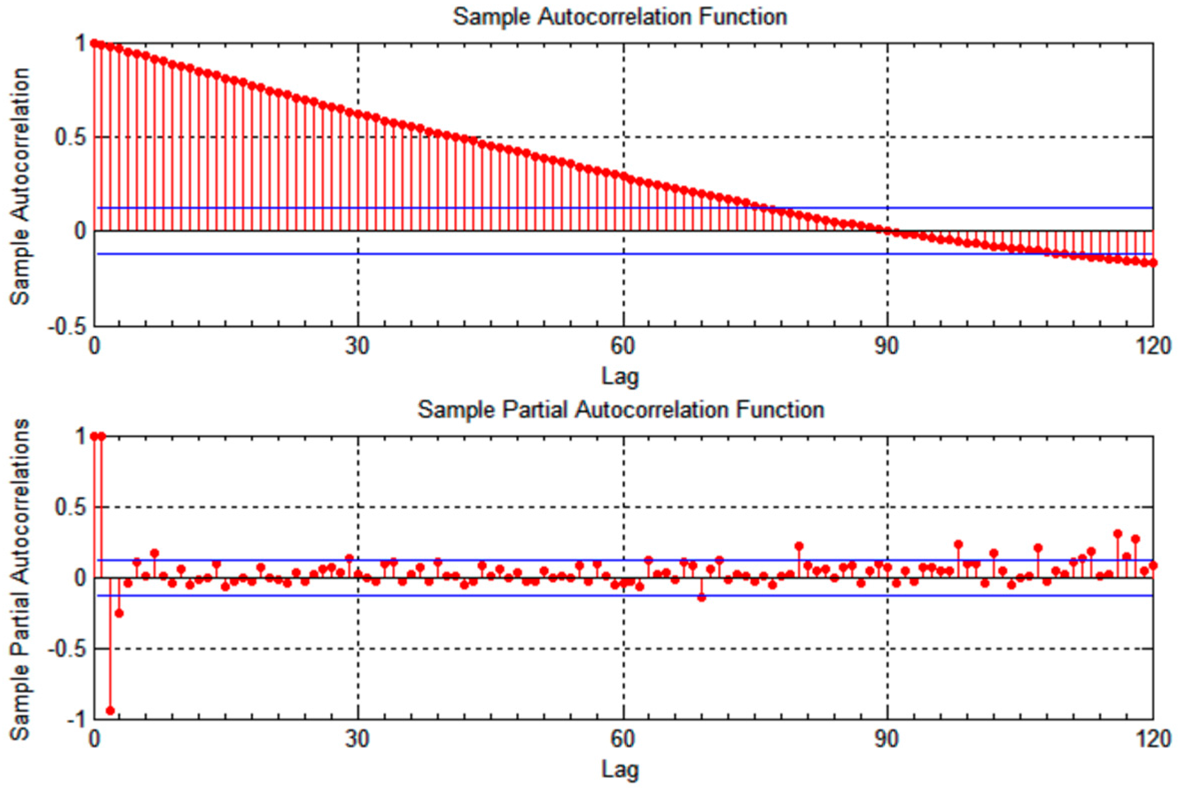
28], and traffic demand was generated using the Travel and Activity PAtterns Simulation (TAPAS) methodology. The original trace covers a region of 400 square kilometers of the city of Cologne for a period of 24 h, comprising more than 700,000 individual car trips. This dataset is the most standardized dataset we could find, with detailed location and speed measurements over a time window that captures most of the traffic patterns that can be experienced in a city with urban and suburban areas. The time granularity between vehicular location measurements is one second, which is reasonable in capturing vehicles’ mobility over time. Vehicle speed varied between 0 km/h and 90 km/h, covering most traffic scenarios. The two-hour excerpt was enough to establish autocorrelation and evaluate its effect on location prediction and error measurements.
The two-hour excerpt trace was preprocessed to extract five traces corresponding to five individual vehicle trips. The five individual vehicles are chosen at random using a uniform distribution-based random number generator, and are labeled
to
throughout the remainder of the paper for ease of reference. A single vehicle trip consists of a time-stamped sequence of
xy position coordinates in meters as well as the vehicle’s speed in meters per second. The selected vehicles’ total trip times are 257 s each. The experiments were conducted using Matlab (R2013a). The estimation of the
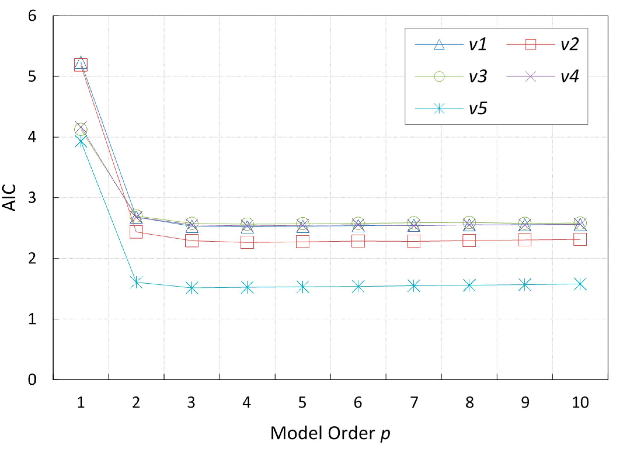
model order was performed using the System Identification Toolbox for
, with the location information for one vehicle used for cross validation. The AIC values for the estimated model were compared for the five vehicles and the majority of them exhibited a best model fit at
, as illustrated in
Figure 5.
We chose two of the five vehicles and used their location measurements to generate the model parameters and validate its performance. The two vehicles used for model estimation and validation were designated
and
, respectively. The location measurements for vehicle
were used to infer the model parameters, and the location measurements for vehicle
were used to validate the model performance using the parameters generated by
’s measurements. We estimated the unknown model coefficients and noise variance for
for the location information of both vehicles using the Yule Walker equations.
5.2. Simulation Results
Three sets of experiments were conducted to investigate two modes of operation for the proposed model. First, we investigated the model performance when used as a standalone model for prediction, for example when GPS is not available. Second, we investigated the performance of our model when integrated into a localization algorithm such as a Kalman filter algorithm. The Kalman filter was chosen because of its popularity as a localization scheme, as well as its ease of implementation. Third, we applied the Kalman filter that was adjusted by the Gauss–Markov model parameters to a real-life dataset in order to assess the accuracy of the enhanced localization scheme and rule out overfitting. The first two sets of experiments study the tradeoff between reducing the complexity of the p-order Gauss–Markov model and the location prediction accuracy, as well as assess the increase in accuracy of localization when using the model in the prediction step of the Kalman filter. The third experiment was used for validation of the model. Each model is designated
for ease of reference.
The model parameters
that were produced by the Yule Walker equations for the two mobility traces for vehicles
and
are listed in
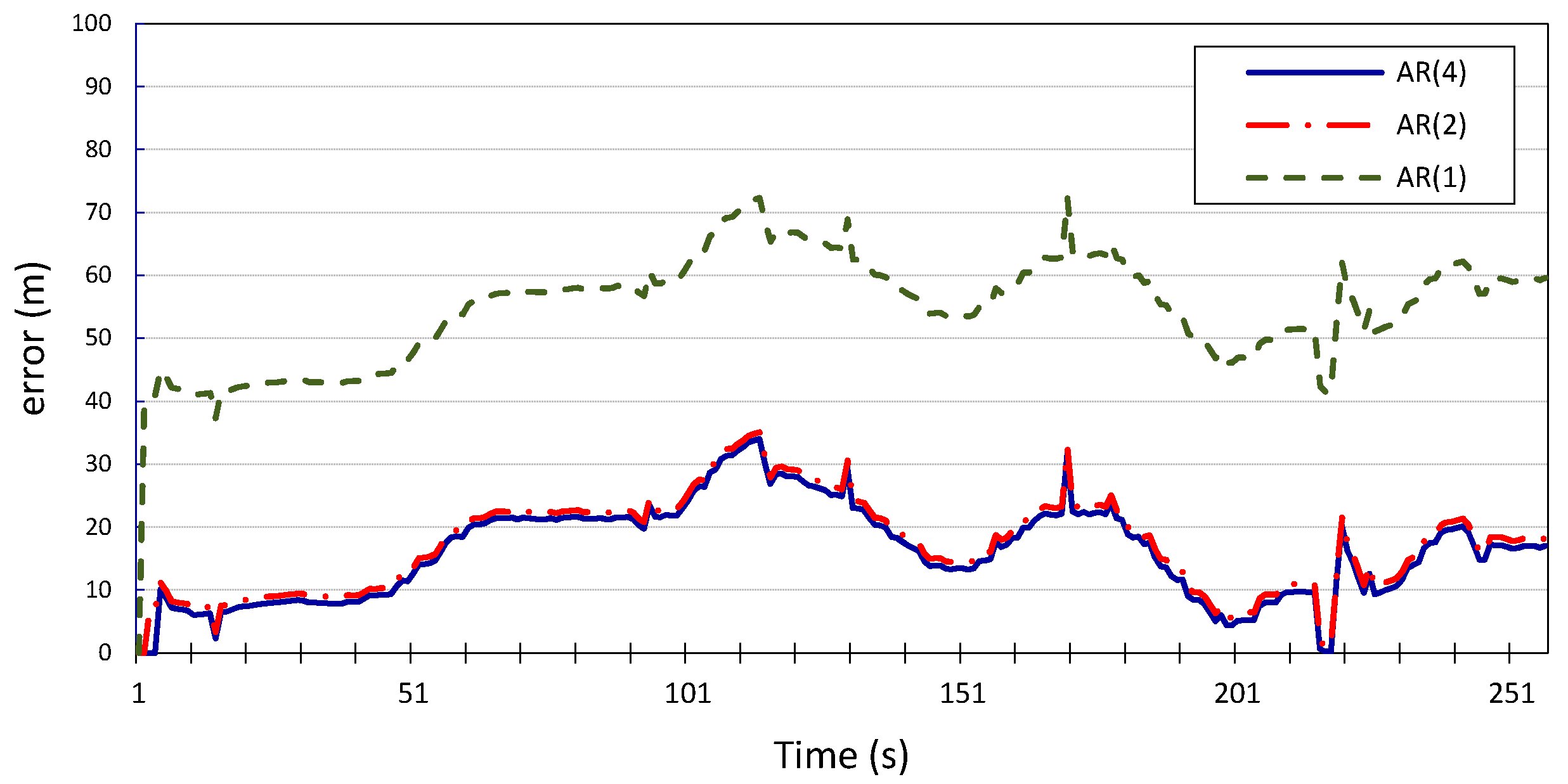
Table 1. For the first set of experiments (standalone prediction), the results in
Figure 6 and
Figure 7 show the errors in the longitudinal (
x) and latitudinal (
y) position estimates made by the Gauss–Markov model for
for vehicle
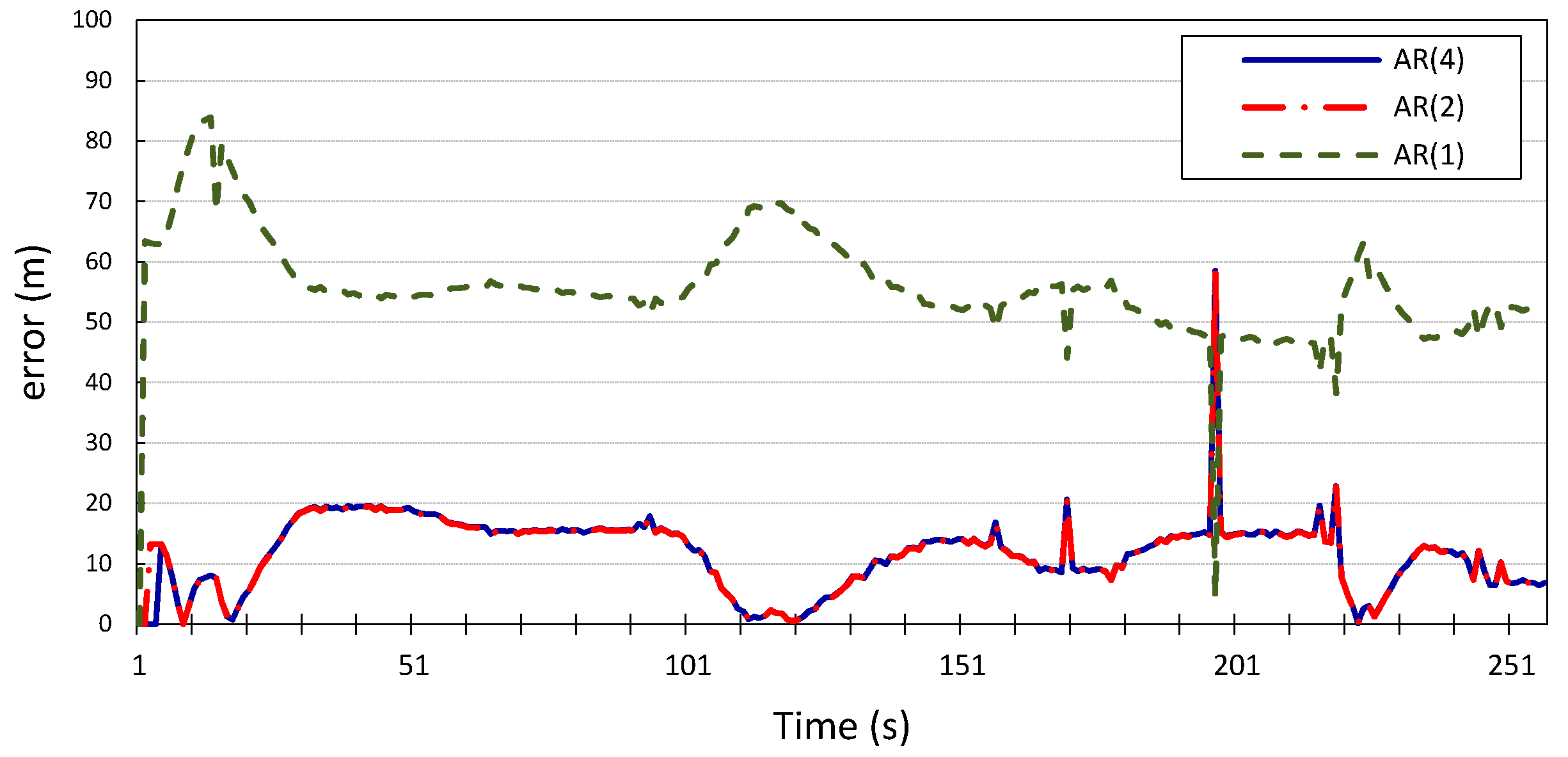
. The figures show that higher model orders correspond to reduced estimation error of the future location coordinates of the vehicle;
and
can predict the vehicle’s location with an average error of 11 m for
x
and 16 m for
y, with inconsiderable improvement made by the model with
compared to the model with
. However, when
, the average error is 55 m for both
x and
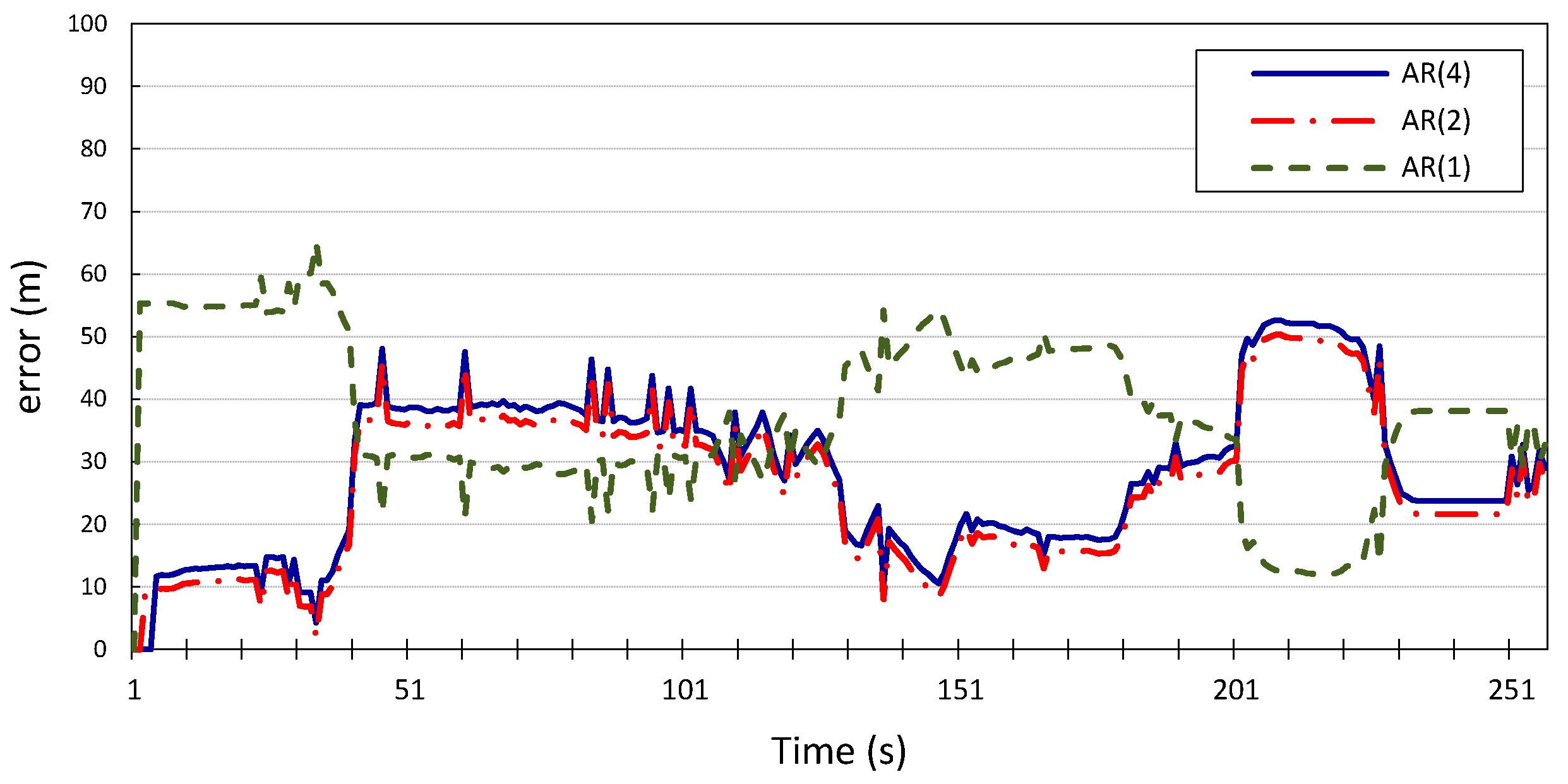
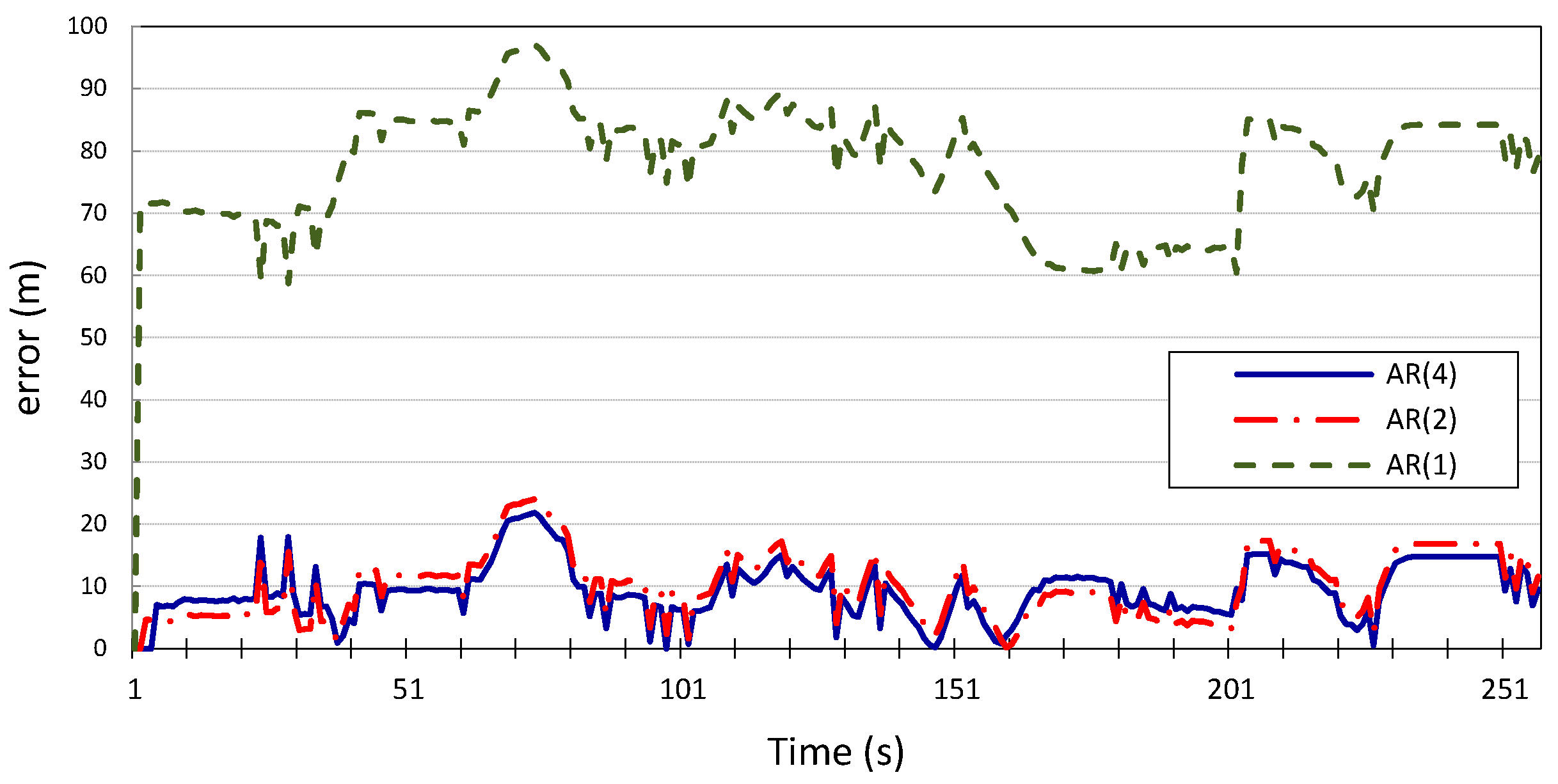
y. This is further corroborated by the results produced when applying the same Gauss–Markov model on the location measurements of vehicle
, which has been designated for validation, as shown in
Figure 8 and
Figure 9. We can conclude that
is a reasonable compromise between complexity and accuracy and therefore is sufficient for depolyment of the error model as a standalone prediction tool. The tradeoff performance provided by the model when
will make the model’s prediction robust even when used in fast-fading channel scenarios, which may exhibit lower correlation windows, since the correlation window in this case is small enough to allow for correlation to be manifested, while still producing accurate prediction. This makes the model applicable in different scenarios with potentially varying correlation windows.
Table 1.
Autoregression model parameters for the two vehicle mobility traces used for experiments.
Table 1.
Autoregression model parameters for the two vehicle mobility traces used for experiments.
| Vehicle Traces | Model | Longitude | Latitude |
|---|
| A1 | A2 | A3 | A4 | A1 | A2 | A3 | A4 |
|---|
| trace v1 | AR(1) | 0.996 | | | | 0.9961 | | | |
| AR(2) | 0.9978 | 0.0018 | | | 0.9977 | 0.0016 | | |
| AR(4) | 0.9978 | 0 | 0 | 0.0018 | 0.9977 | 0.0001 | 0 | 0.0016 |
| trace v2 | AR(1) | 0.9963 | | | | 0.996 | | | |
| AR(2) | 0.9992 | 0.0029 | | | 0.9976 | 0.0016 | | |
| AR(4) | 0.9992 | 0.0001 | 0.0002 | 0.0028 | 0.9976 | 0.0001 | 0.0001 | 0.0015 |
Figure 6.
Longitudinal position error for vehicle v1 using autoregression model with p = 1, 2, 4.
Figure 6.
Longitudinal position error for vehicle v1 using autoregression model with p = 1, 2, 4.
Figure 7.
Latitudinal position error for vehicle v1 using autoregression model with p = 1, 2, 4.
Figure 7.
Latitudinal position error for vehicle v1 using autoregression model with p = 1, 2, 4.
Figure 8.
Longitudinal position error for vehicle v2 using autoregression model with p = 1, 2, 4.
Figure 8.
Longitudinal position error for vehicle v2 using autoregression model with p = 1, 2, 4.
Figure 9.
Latitudinal position error for vehicle v2 using autoregression model with p = 1, 2, 4.
Figure 9.
Latitudinal position error for vehicle v2 using autoregression model with p = 1, 2, 4.
For the second experiment, we want to investigate the integration of the model into a localization algorithm. The Gauss–Markov model was integrated into the Kalman filter localization scheme proposed in [
29] in order to illustrate how error modeling and parameter estimation enhance the accuracy of localization. We will experiment with
to assess whether reducing the model complexity using
will provide comparable results to higher orders.
The Kalman filter involves two steps: a prediction step and a measurement update step. The prediction step assumes that the state of a system at time
t evolved from the prior state at
according to:
where
is the state vector containing system information at time
t,
is a vector containing control inputs,
is a state transition matrix that applies the effects of the system state at
to its state at time
t,
Bt is a control input matrix that serves a similar purpose to
Ft but for the control inputs, and
is the process noise. In our experiments, the transition matrix
was composed using the parameter values
that were produced by the Yule Walker equations, which are listed in
Table 1. A different matrix was constructed for each model using the longitude and latitude parameter values. The size of the transformation matrix was the same size of the dataset. The control matrix
was set to zero since there are no control inputs. The measurement step performs corrections to the predicted location, according to the equation:
where
is the vector of measurements,
is a transformation matrix which is set to default value of 1 in our experiments, and
represents the measurement noise.
The process and measurement noise in Kalman filter-based localization algorithms are usually assumed to be zero-mean Gaussian white noise. Our proposed error model can compute the noise variance in location information. Therefore, we incorporate it into the prediction step of the Kalman filter and study how this will improve the localization algorithm. The
-integrated Kalman filter is then applied to the two time series location information of vehicles
and
, and the results shown in
Figure 10,
Figure 11,
Figure 12 and
Figure 13 compare the localization error for the three error models;
,
, and
. We note that the computational complexity of the Kalman filter and the
autoregression-integrated Kalman filter is dominated by the matrix multiplication, and therefore grows as
, where
is the number of location measurements. We also note that the computational complexity of the AR-integrated Kalman filter implementation and the standard Kalman filter implementation are identical. This is because the integration of the AR model into the Kalman filter involves the replacement of the transition and error matrices and the extension of prediction step to accommodate computations when
and
.
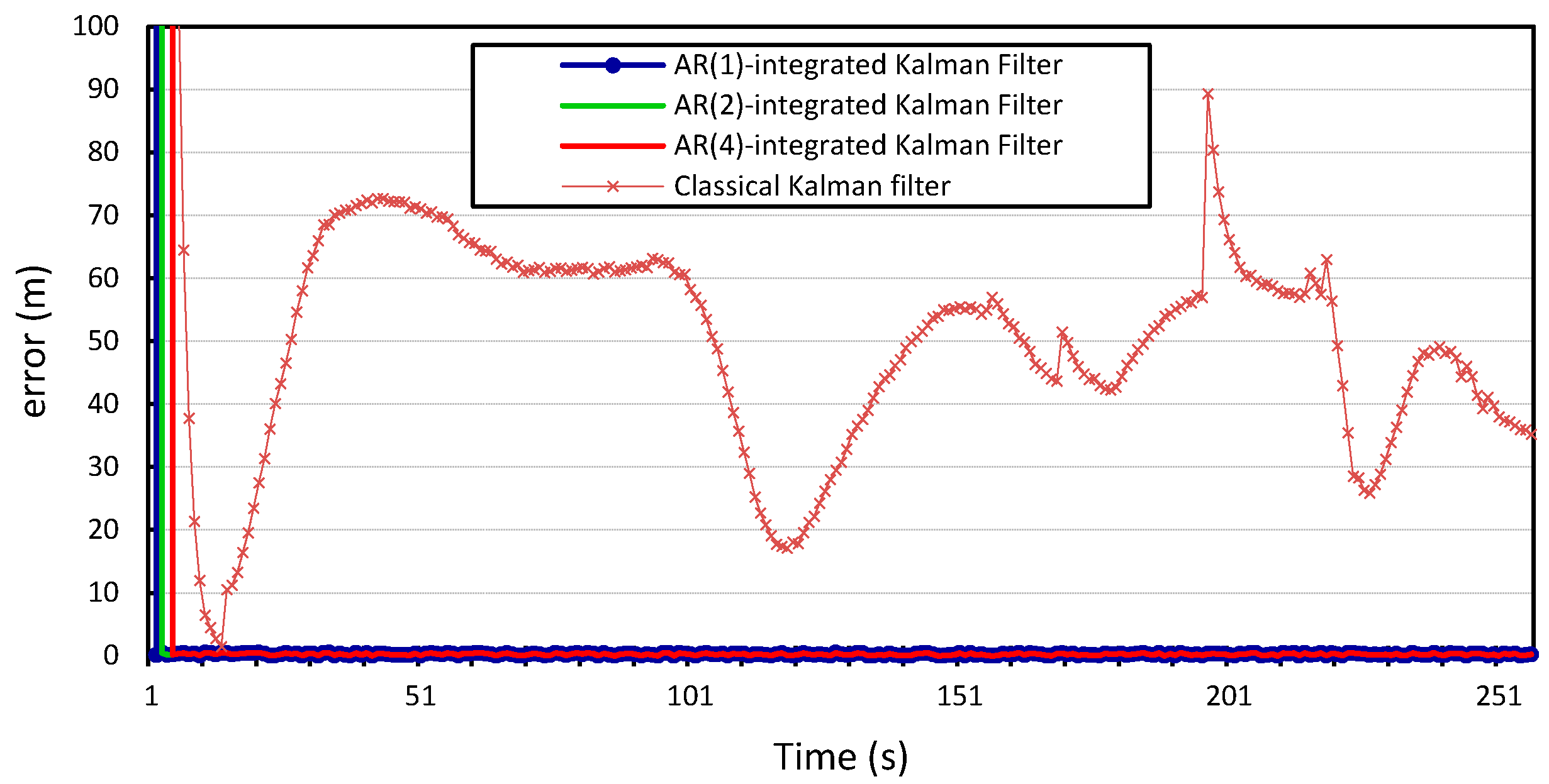
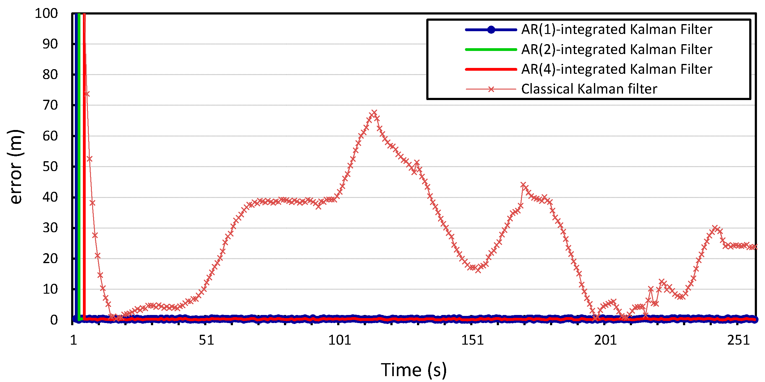
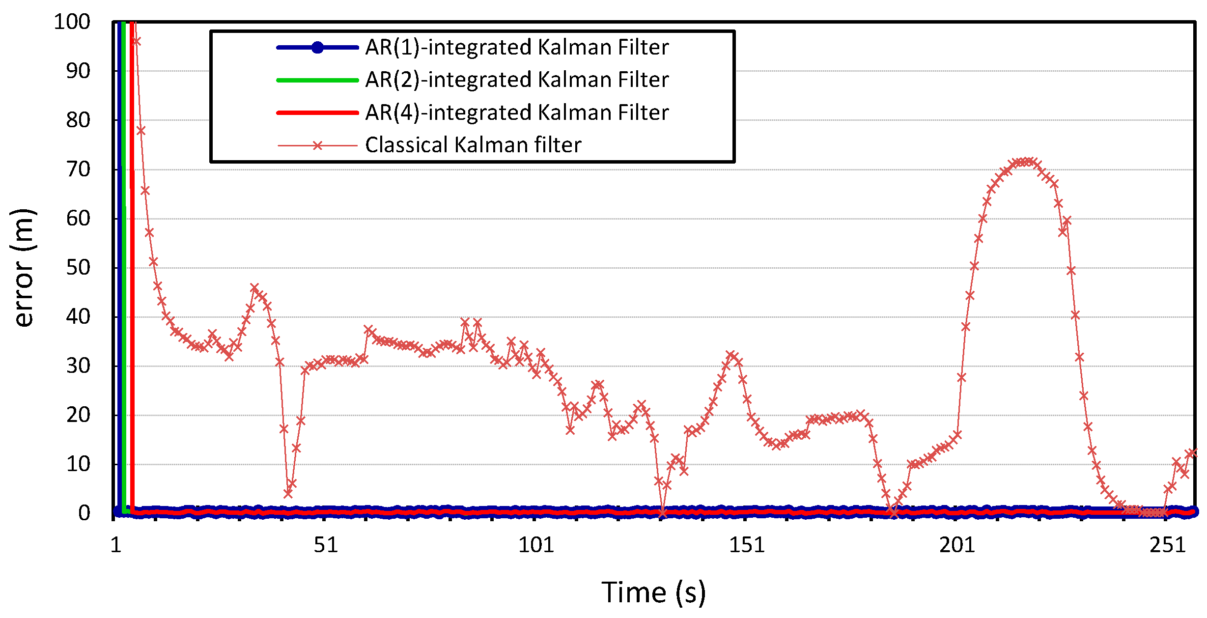
We can see that incorporating our error model into the Kalman filter outperforms the results produced by the Kalman filter with zero Gaussian error, which we call the standard Kalman filter for convenience. Similar accuracy gains are obtained when the error model is integrated into the Kalman filter and applied to the location measurements of vehicle
whose location information is used for validation. We can also observe that there is no observable gain in accuracy when using a higher Gauss–Markov order, since
provides almost identical results to
. The average measurement error for the standard Kalman filter applied to the location measurements of vehicle
is 56 m and 29 m for
x and
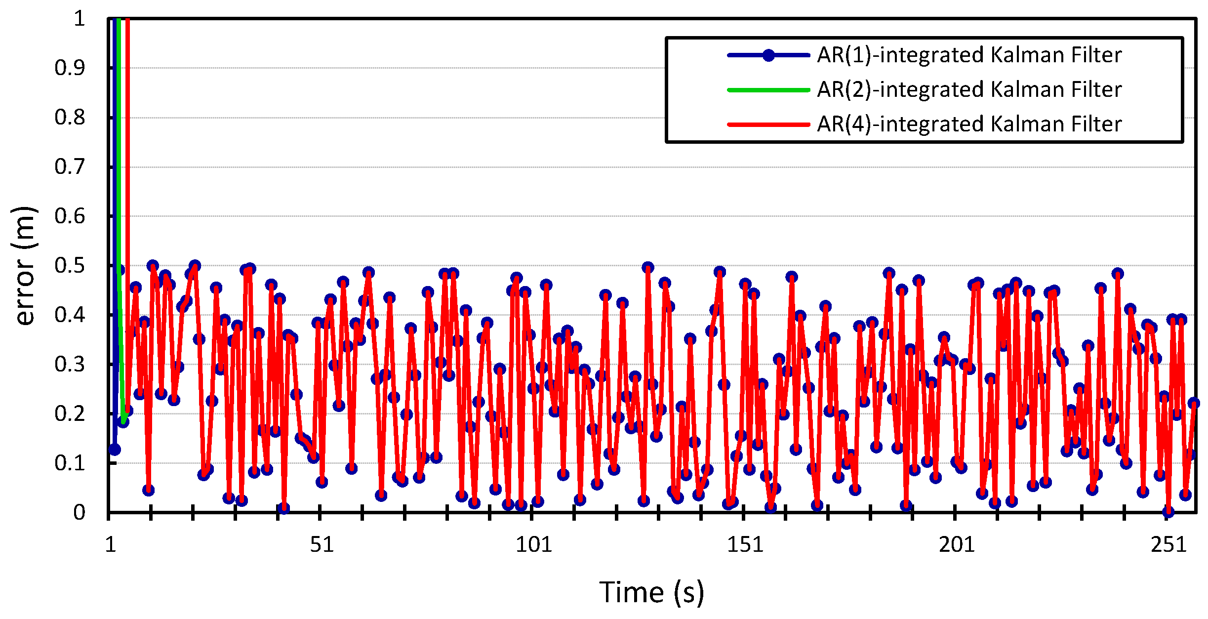
y, respectively, compared to 0.25 m produced by the Kalman filter that is integrated with the autoregression model of order 1. The Kalman filter that was integrated with the autoregression model of order 4 has an average measurement error of 0.24 m, which is very close to that produced by the autoregression model of order 1. This can be further illustrated in
Figure 14 and
Figure 15, which provide a more detailed view of the behavior of the model for
. The fluctuations in error measurements are due to the constant variability in the vehicles’ position measurements, as was found upon further inspection of the original time-series for longitudinal and latitudinal location measurements of both vehicles.
Figure 10.
Longitudinal positioning error produced by the standard Kalman filter and the Autoregression-Kalman filter for vehicle
.
Figure 10.
Longitudinal positioning error produced by the standard Kalman filter and the Autoregression-Kalman filter for vehicle
.
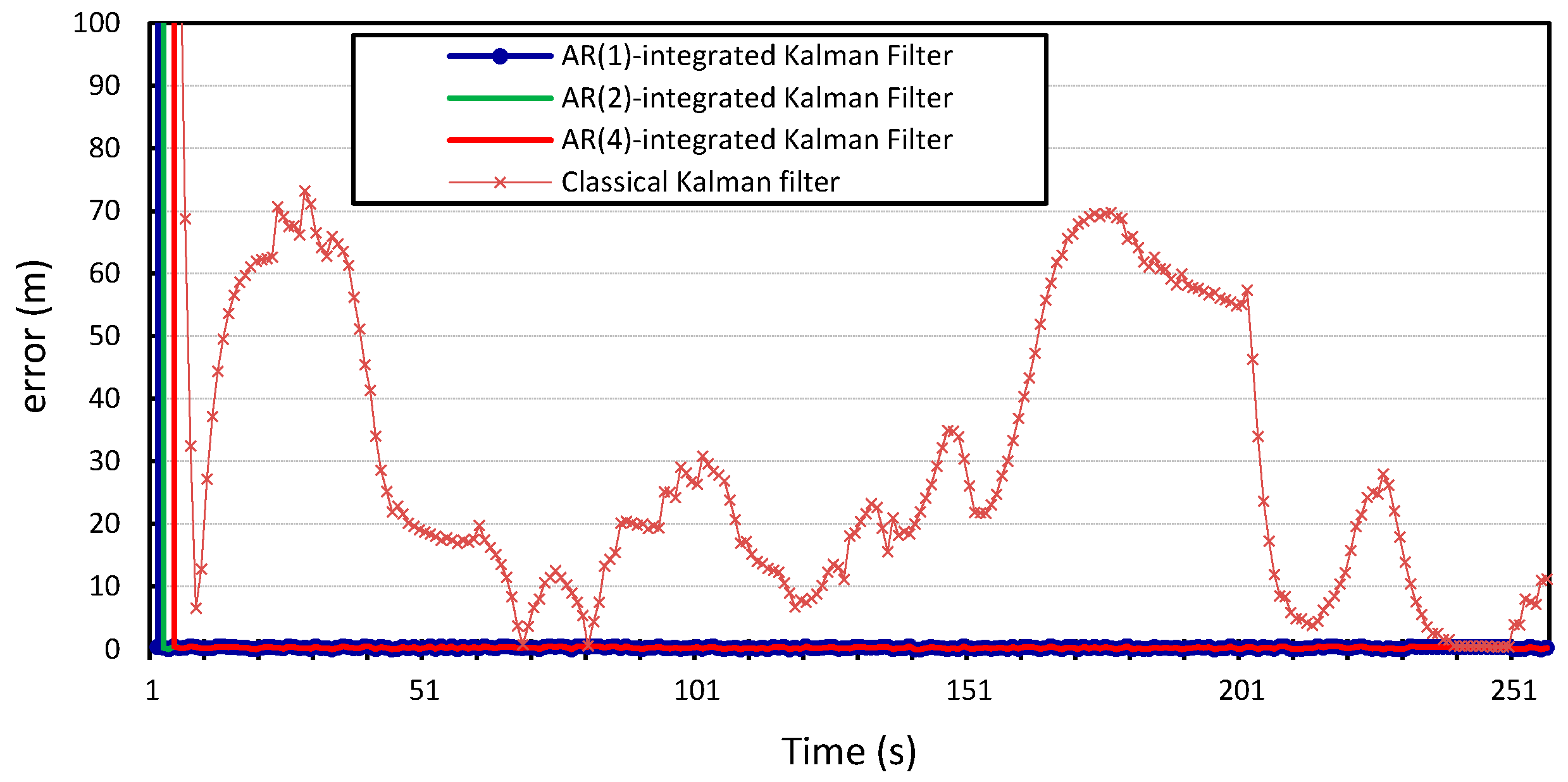
Figure 11.
Latitudinal positioning error produced by the standard Kalman filter and the Autoregression-Kalman filter for vehicle
.
Figure 11.
Latitudinal positioning error produced by the standard Kalman filter and the Autoregression-Kalman filter for vehicle
.
Figure 12.
Longitudinal positioning error produced by the standard Kalman filter and the Autoregression-Kalman filter for vehicle
.
Figure 12.
Longitudinal positioning error produced by the standard Kalman filter and the Autoregression-Kalman filter for vehicle
.
Figure 13.
Latitudinal positioning error produced by the standard Kalman filter and the Autoregression-Kalman filter for vehicle
.
Figure 13.
Latitudinal positioning error produced by the standard Kalman filter and the Autoregression-Kalman filter for vehicle
.
Figure 14.
Zoom in on the longitudinal positioning error produced by the Autoregression-Kalman filter for vehicle
.
Figure 14.
Zoom in on the longitudinal positioning error produced by the Autoregression-Kalman filter for vehicle
.
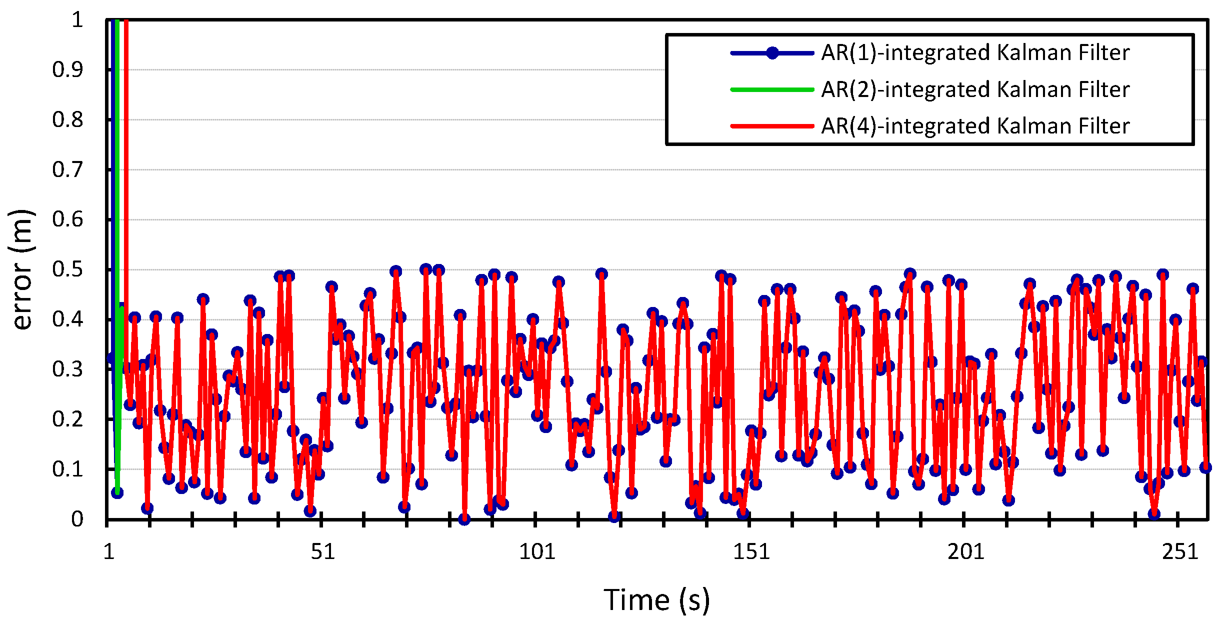
Figure 15.
Zoom in on the latitudinal positioning error produced by the Autoregression-Kalman filter for vehicle
.
Figure 15.
Zoom in on the latitudinal positioning error produced by the Autoregression-Kalman filter for vehicle
.
5.3. Verification of Model
In order to verify our
model, we tested the model against three realistic datasets. We chose three vehicular mobility traces from OpenStreetMap [
30]. The first trace (
), which is illustrated in
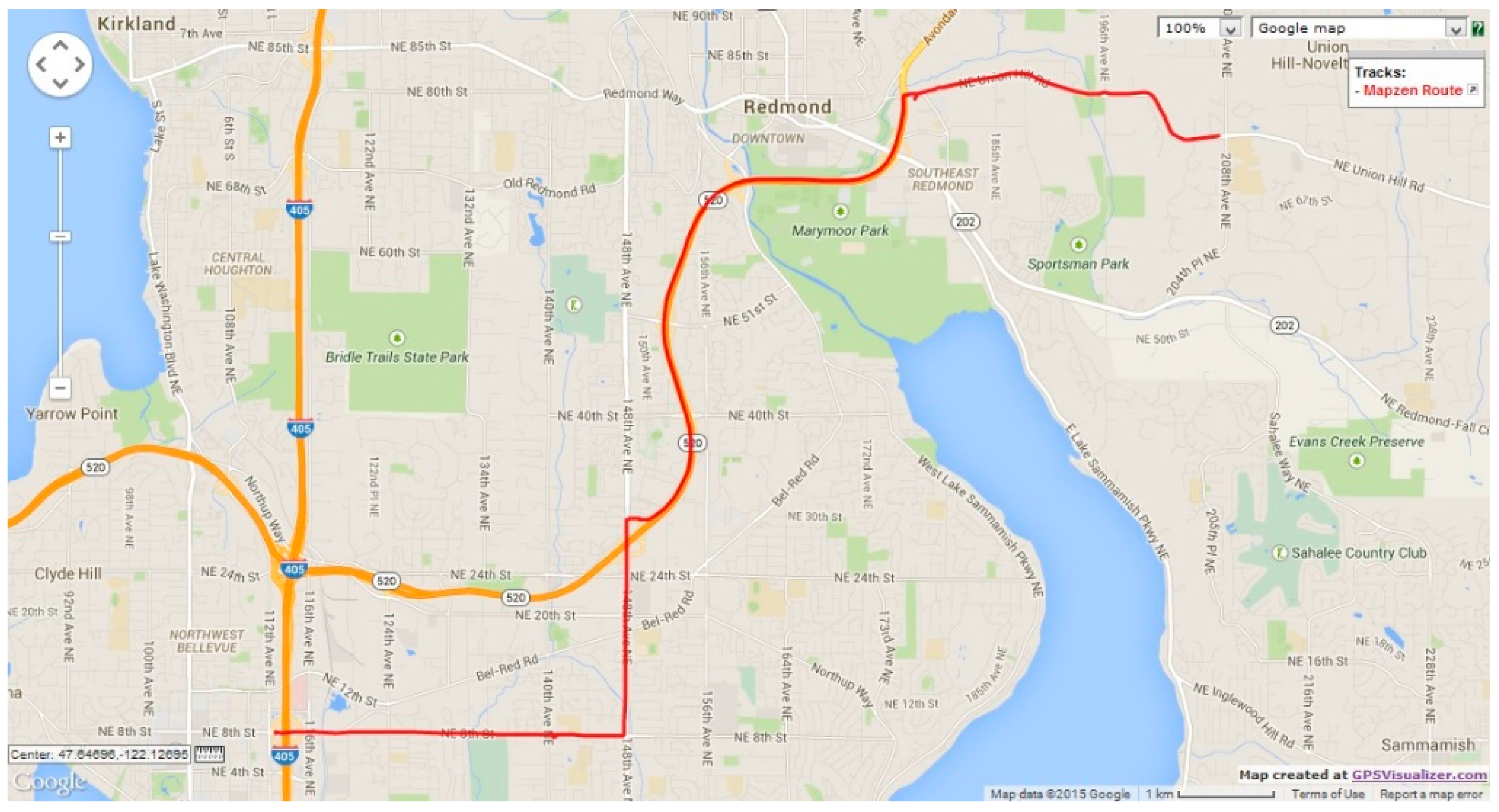
Figure 16, represents a single vehicle trip along the route between Northeast Union Hill Road and Bravern 1, Bellevue, WA. The total trip time was 30 min and 45 s (totaling 1845 data points), and vehicle speed ranged from 0 km/h to 104.4 km/h. The second trace (
), illustrated in
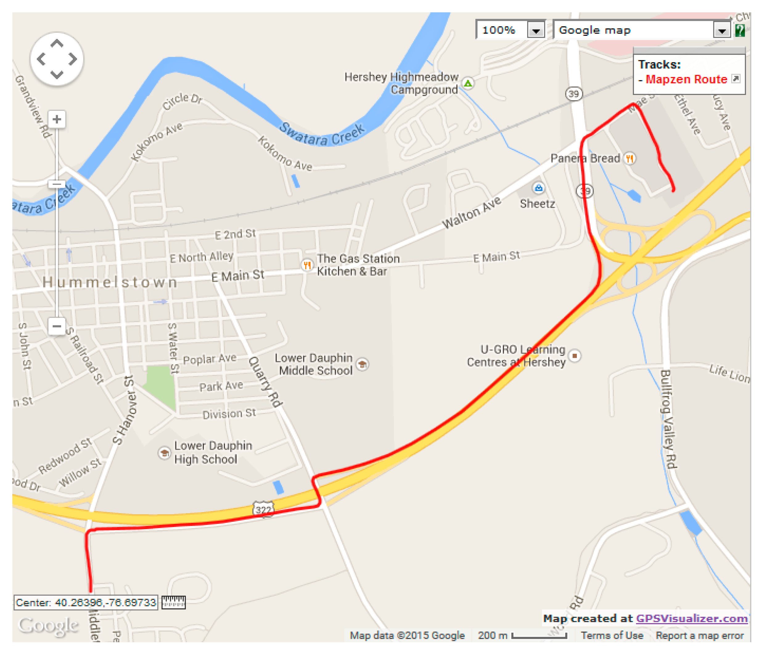
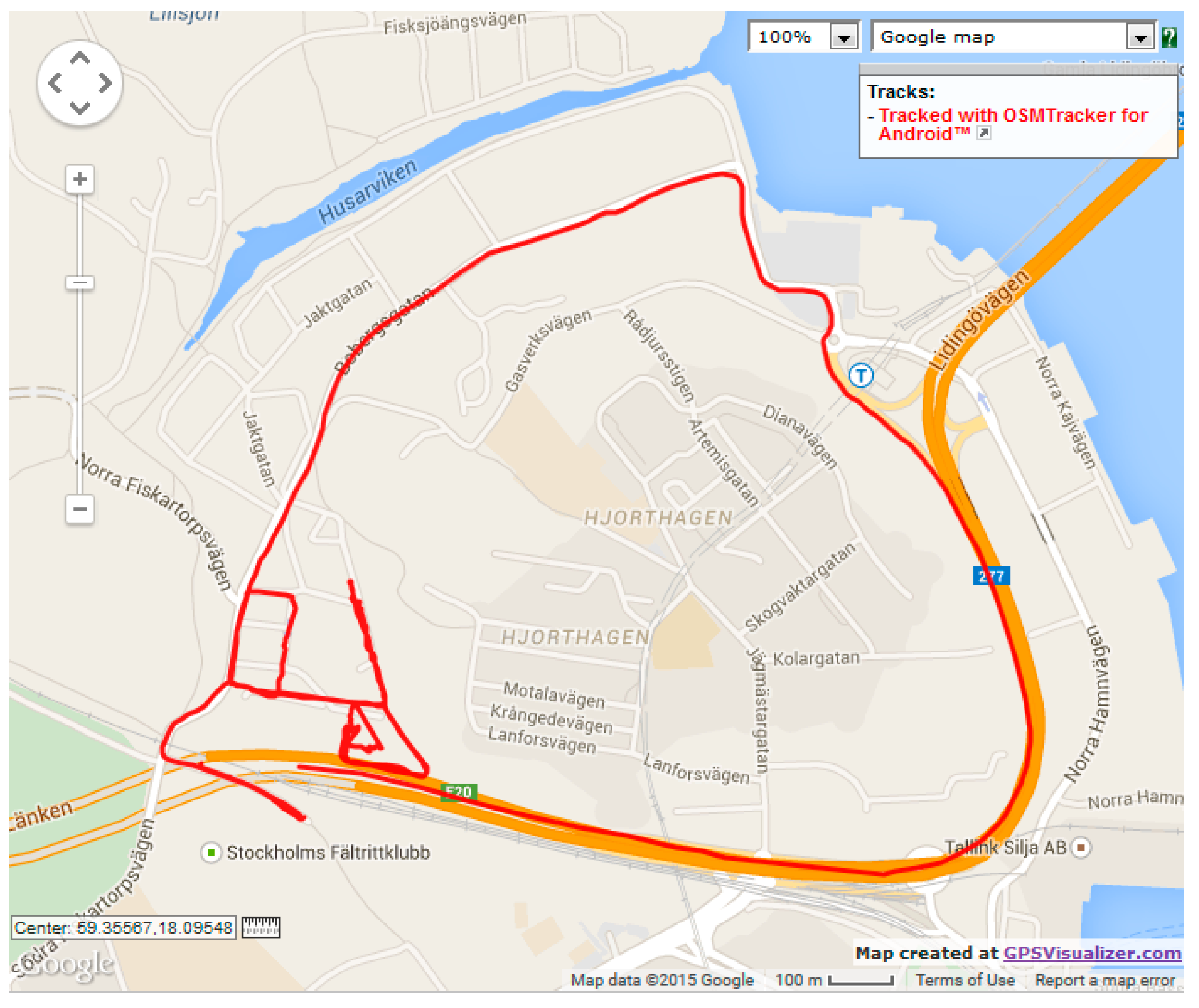
Figure 17, represents a single vehicle trip between East Main Street and the Gelder Park, Derry, PA, USA. The total trip time was 5 min and 45 s (totaling 343 data points), and speed ranged from 0 km/h to 96.7 km/h. The third trace (
), illustrated in
Figure 18, depicts a vehicle’s trip around a new residential area in Stockholm, Sweden. The total vehicle trip time was 25 min and 56 s (totaling 1313 data points). There is no mention of the vehicle speeds for the third dataset. For the three datasets, location measurements were taken every second.
Figure 16.
OpenStreetMap route for verification dataset 1.
Figure 16.
OpenStreetMap route for verification dataset 1.
Figure 17.
OpenStreetMap route for verification dataset 2.
Figure 17.
OpenStreetMap route for verification dataset 2.
Figure 18.
OpenStreetMap route for verification dataset 3.
Figure 18.
OpenStreetMap route for verification dataset 3.
As with the previous experiment set, the model parameters and process noise were extracted from each of the datasets using the autoregression model of order 1. The Kalman filter was integrated with the model parameters and applied to the location measurements.
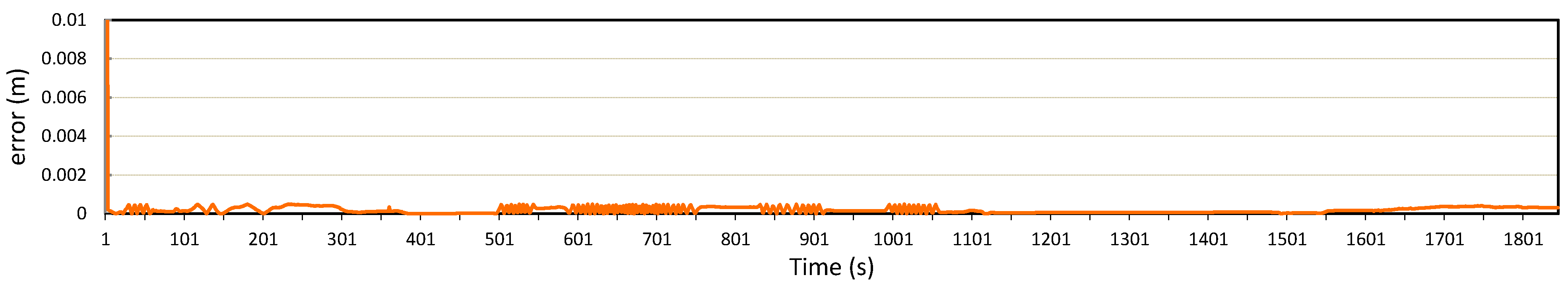
Figure 19,
Figure 20,
Figure 21,
Figure 22,
Figure 23 and
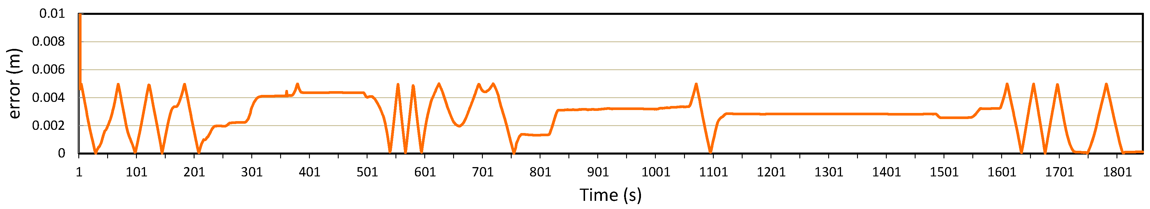
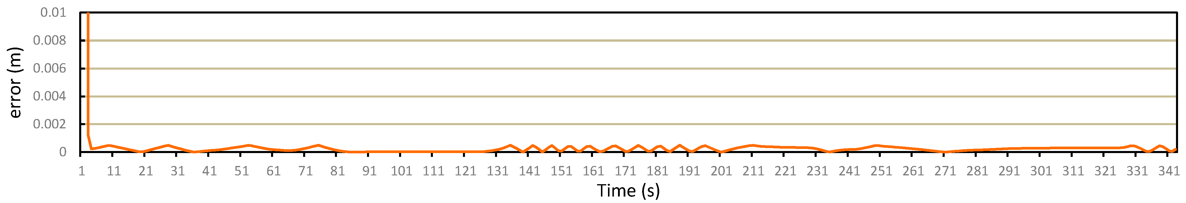
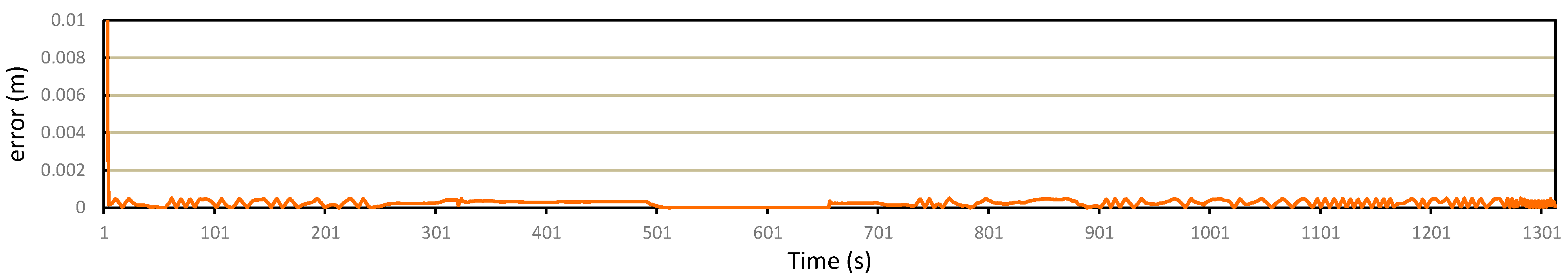
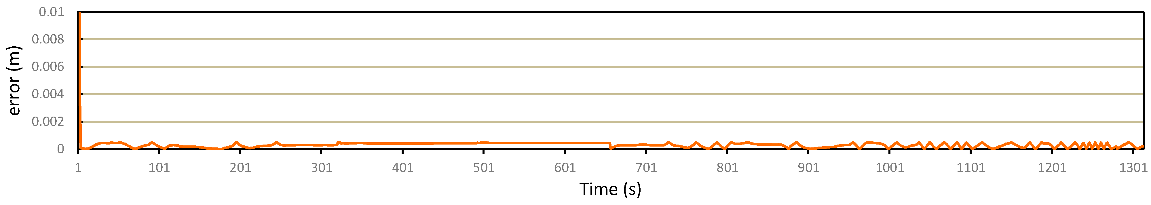
Figure 24 show, respectively, the longitudinal and latitudinal position measurement errors produced by the Kalman filter when the Gauss–Markov model is used for the prediction step when applied to the OpenStreetMap traces. The margin of error for all three datasets stays within a very small and negligible range (0.005 m), which indicates the high level of accuracy produced by the localization model. The larger variation in longitudinal error in comparison to the latitudinal error in
is due to the larger variation rate in longitudinal measurements compared to a small overall change in the latitudinal measurements.
The localization model performs well regardless of the road scenario—highway, residential, or a combination of both. Error variation is miminal at the intervals during which the vehicles do not change their positions, as can be noticed in the interval between the seconds 1101 and 1550 in
and between the seconds 310 and 650 for
, for example. We notice that error in the third section of the position measurements for
exhibits more fluctuations. When the corresponding vehicle’s route is closely inspected, it can be evident that this variation is due to the rather unsmooth movement along some sections of the residential area. We can assume that this error variation can be controlled if vehicle speed is incorporated into the prediction model, which is part of our future work.
Figure 19.
Longitudinal positioning error produced by Autoregression-Kalman filter for dataset 1.
Figure 19.
Longitudinal positioning error produced by Autoregression-Kalman filter for dataset 1.
Figure 20.
Latitudinal positioning error produced by Autoregression-Kalman filter for dataset 1.
Figure 20.
Latitudinal positioning error produced by Autoregression-Kalman filter for dataset 1.
Figure 21.
Longitudinal positioning error produced by Autoregression-Kalman filter for dataset 2.
Figure 21.
Longitudinal positioning error produced by Autoregression-Kalman filter for dataset 2.
Figure 22.
Latitudinal positioning error produced by Autoregression-Kalman filter for dataset 2.
Figure 22.
Latitudinal positioning error produced by Autoregression-Kalman filter for dataset 2.
Figure 23.
Longitudinal positioning error produced by Autoregression-Kalman filter for dataset 3.
Figure 23.
Longitudinal positioning error produced by Autoregression-Kalman filter for dataset 3.
Figure 24.
Latitudinal positioning error produced by Autoregression-Kalman filter for dataset 3.
Figure 24.
Latitudinal positioning error produced by Autoregression-Kalman filter for dataset 3.


