
Daytime Land Surface Temperature Extraction from MODIS Thermal Infrared Data under Cirrus Clouds


Abstract
:1. Introduction
2. Data
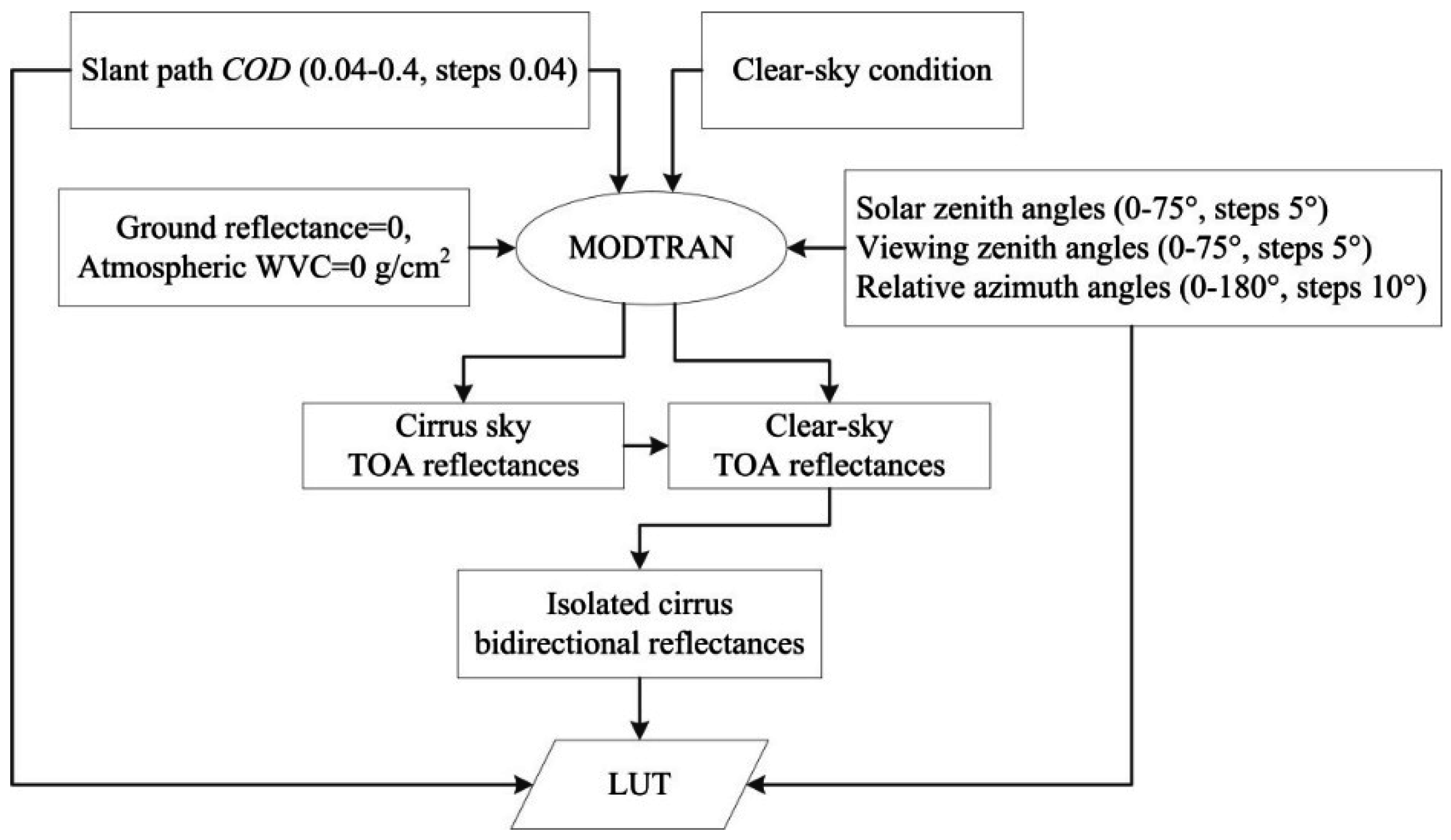
2.1. Simulated Datasets
2.2. Satellite Data
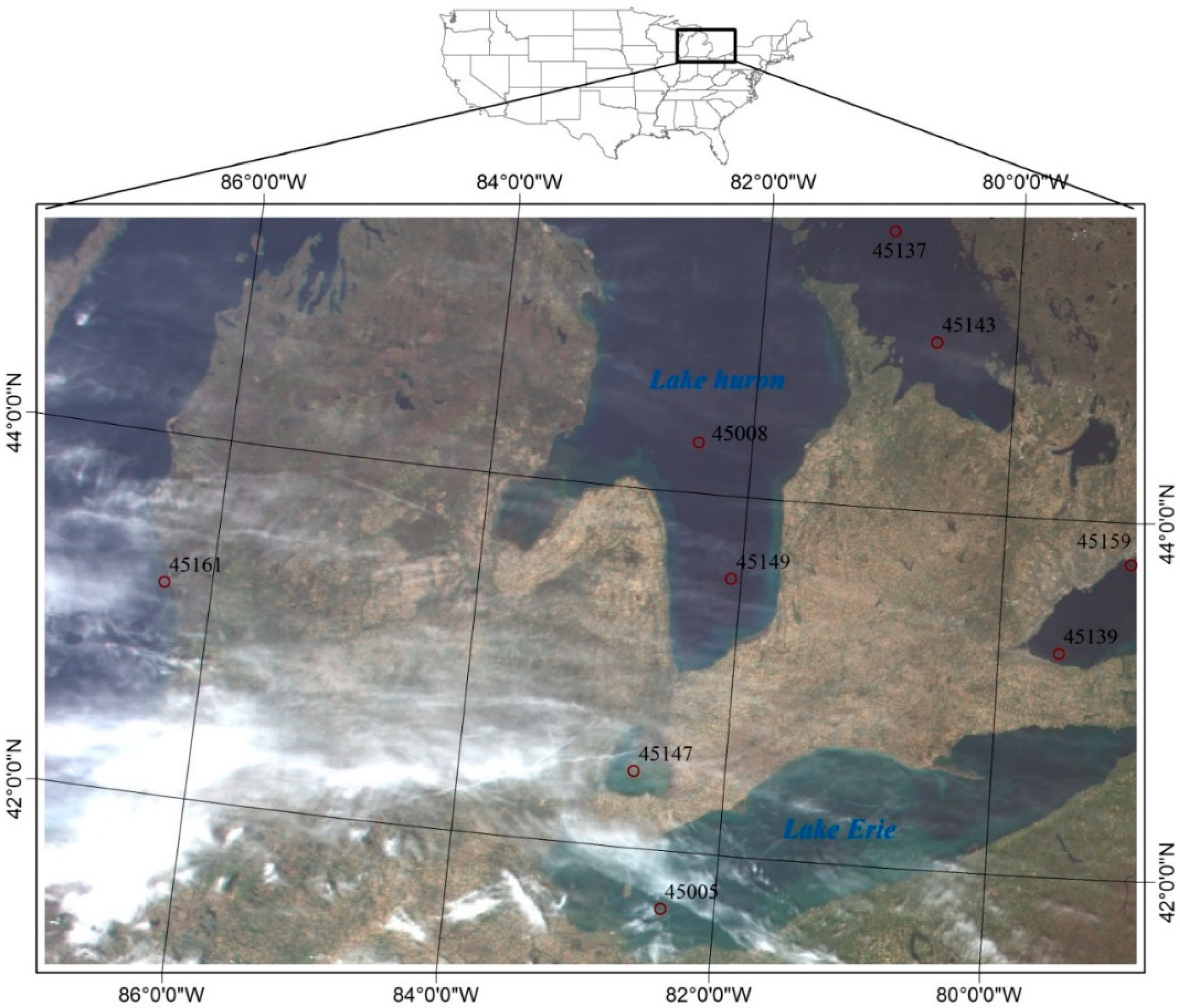
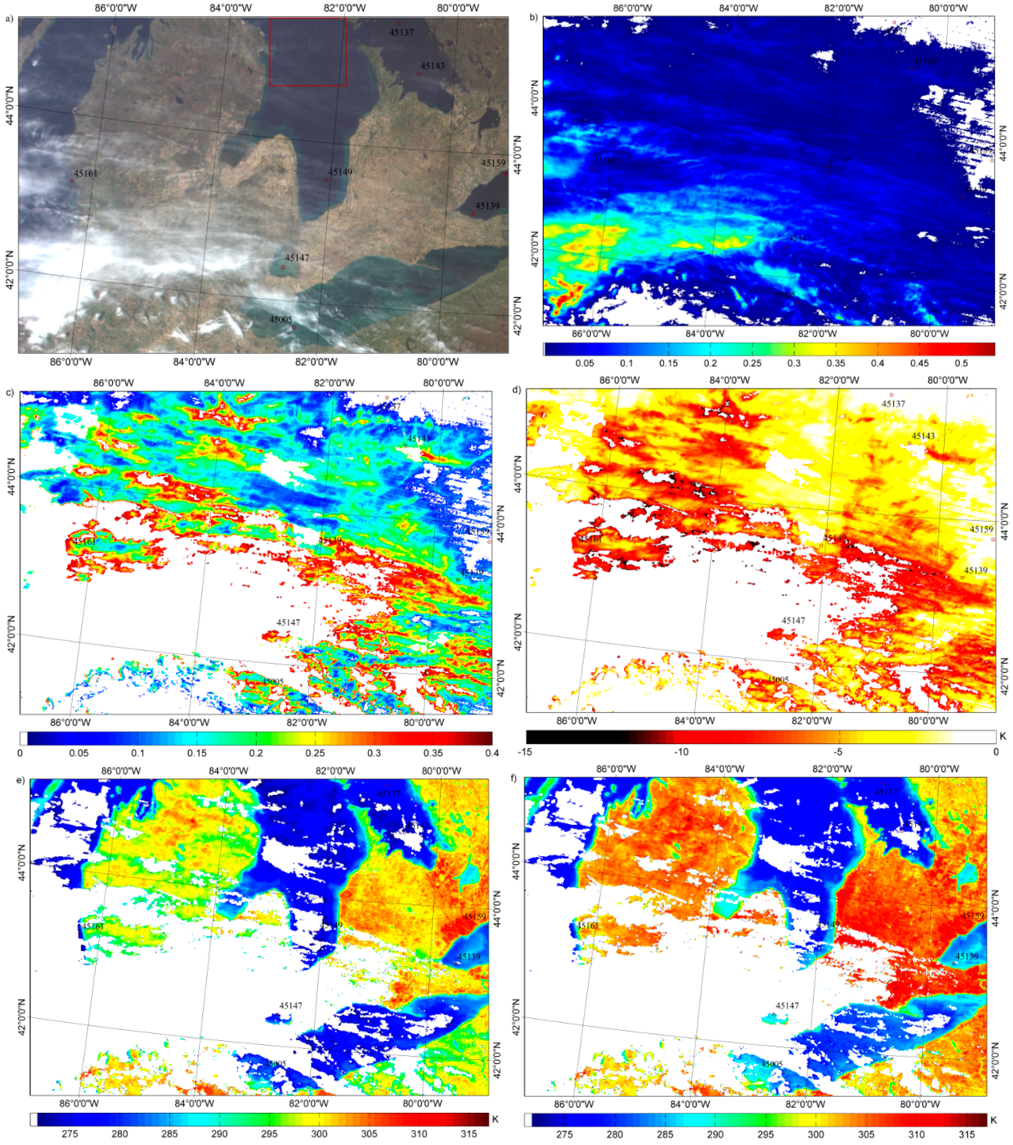
2.3. Study Area and Field Measurements
3. Method
3.1. LST Retrieval under Cirrus Clouds
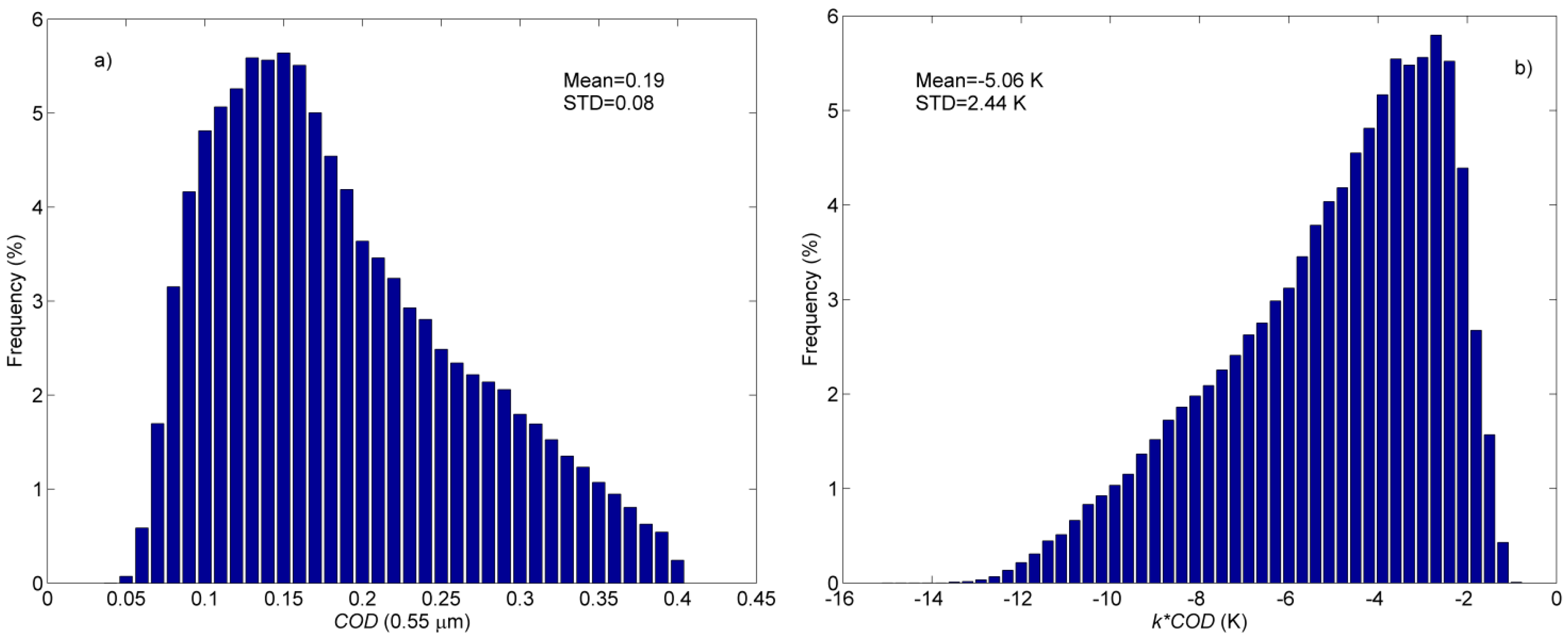
3.2. Determination of Slope k
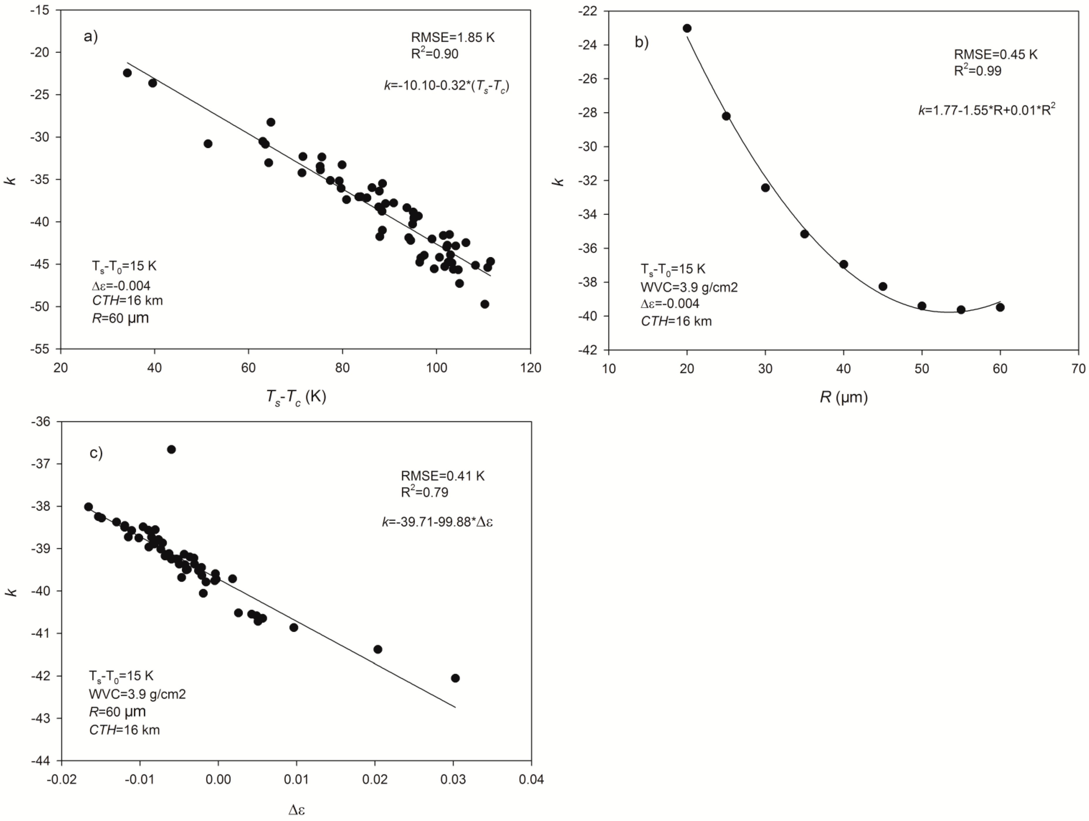

| Secant(VZA) | k0 (K) | k1 | k2 | k3 | k4 (K) | RMSE (K) |
|---|---|---|---|---|---|---|
| 1.0 | −17.57 | 0.67 | −1.39 | −1.09 | −37.85 | 5.67 |
| 1.2 | −20.38 | 0.97 | −1.73 | −1.48 | −27.90 | 6.41 |
| 1.4 | −21.37 | 0.92 | −1.58 | −2.21 | −13.11 | 7.01 |
| 1.6 | −22.28 | 0.92 | −1.51 | −2.74 | −3.18 | 7.47 |
| 1.8 | −22.86 | 0.89 | −1.44 | −3.18 | 4.47 | 7.87 |
| 2.0 | −22.84 | 0.72 | −1.16 | −3.8 | 12.92 | 8.33 |
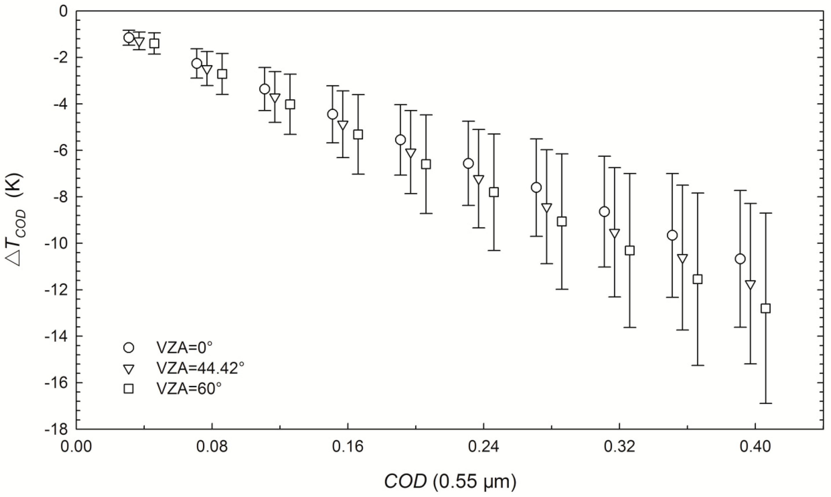
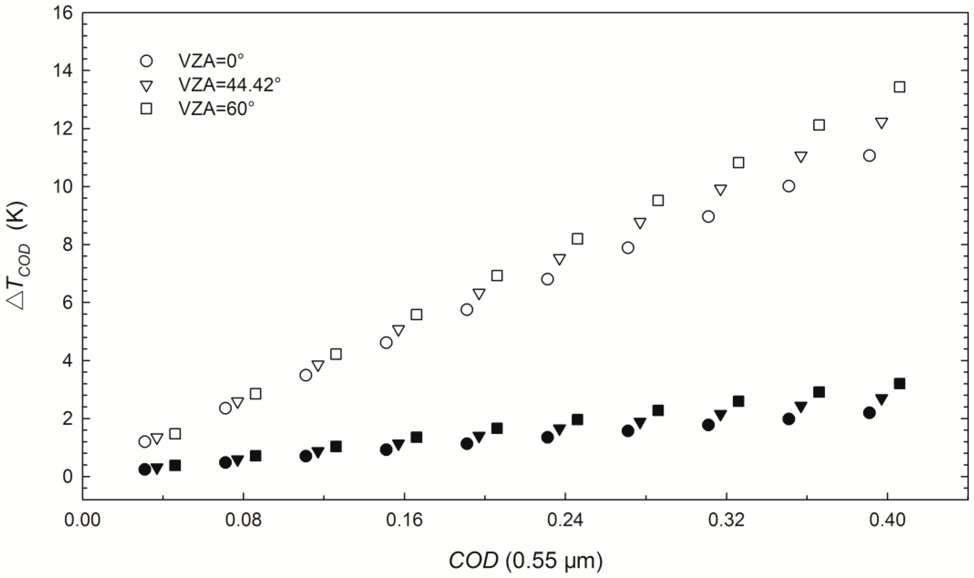
3.3. Determination of COD

4. Results and Analysis
4.1. Results

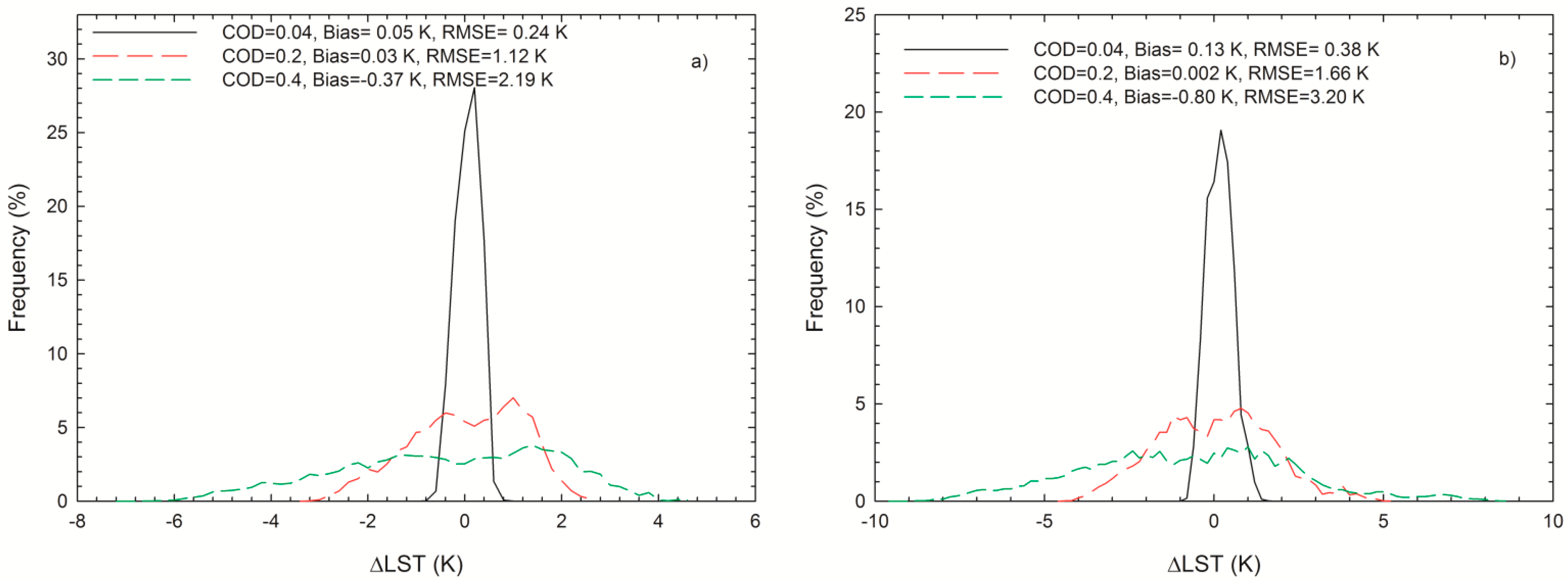
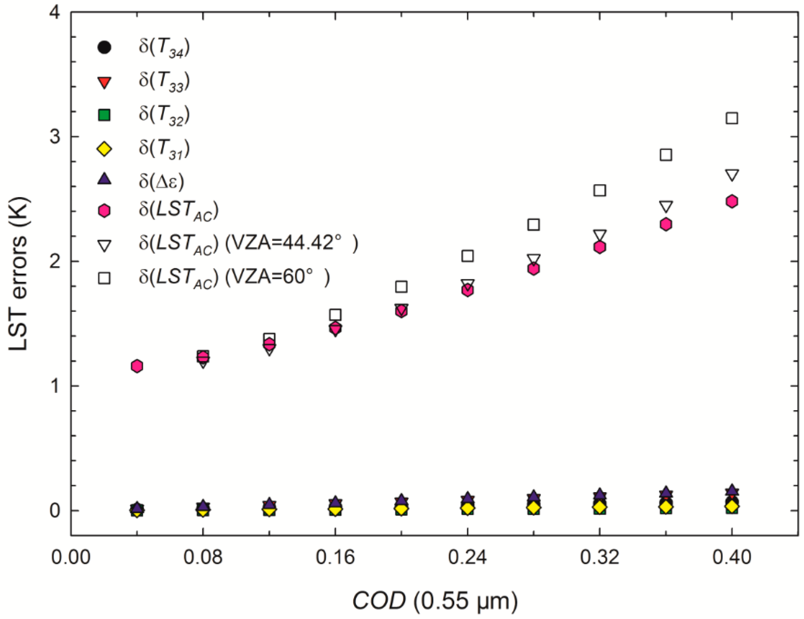
4.2. Analysis

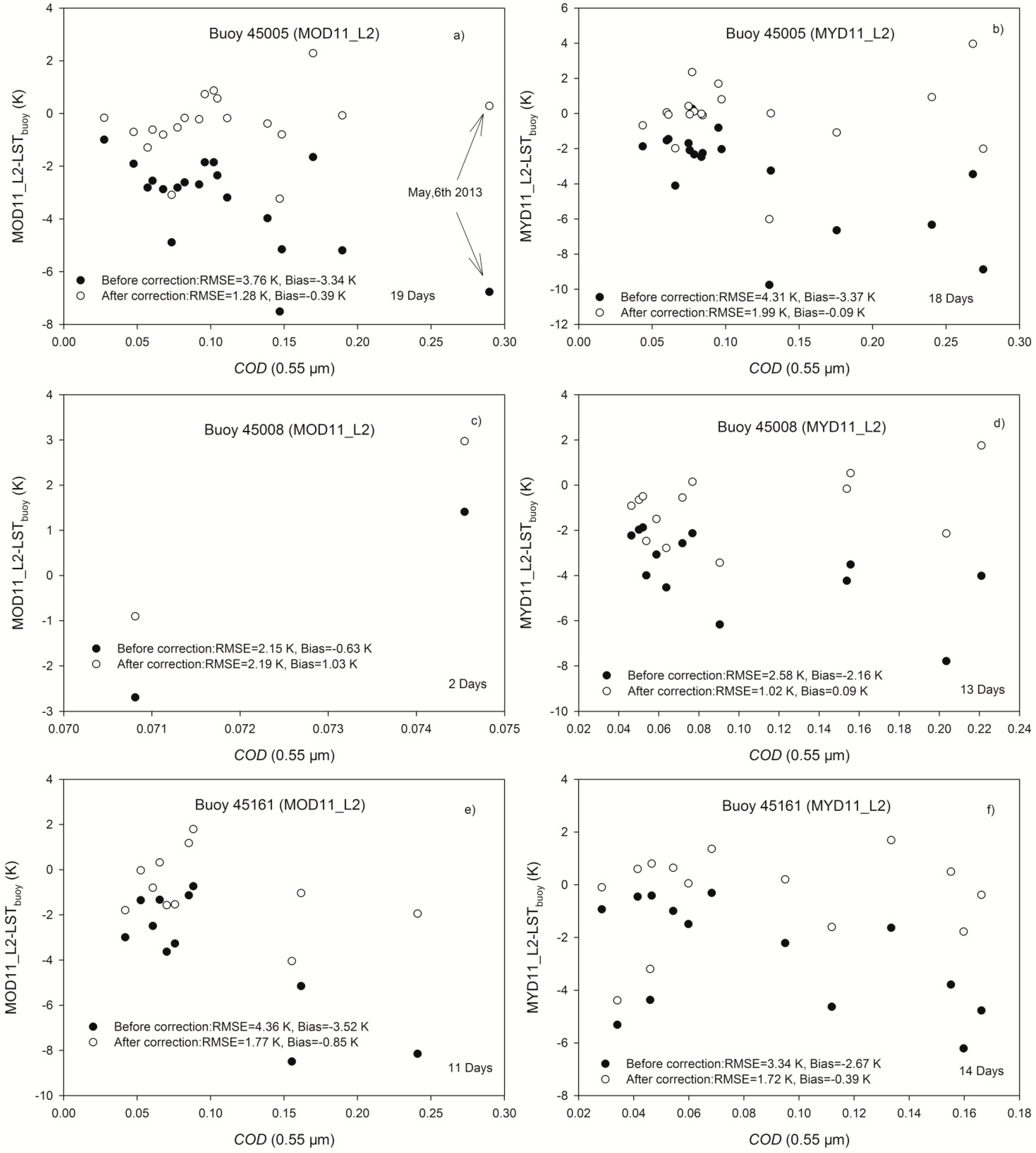
5. Validations

| Data | Days | MOD11_L2/ MY11_L2 | LSTAC | ||
|---|---|---|---|---|---|
| Bias (K) | RMSE (K) | Bias (K) | RMSE (K) | ||
| 45137/MOD11_L2 | 0 | - | - | - | - |
| 45137/MYD11_L2 | 5 | −2.94 | 3.49 | 2.05 | 4.68 |
| 45139/MOD11_L2 | 4 | −4.71 | 5.67 | −3.37 | 4.88 |
| 45139/MYD11_L2 | 3 | −3.19 | 3.26 | −0.35 | 1.10 |
| 45143/MOD11_L2 | 3 | −2.10 | 2.28 | 1.71 | 3.40 |
| 45143/MYD11_L2 | 9 | −1.54 | 1.67 | 1.55 | 3.44 |
| 45147/MOD11_L2 | 5 | −5.77 | 6.05 | 0.35 | 2.34 |
| 45147/MYD11_L2 | 1 | −1.95 | - | 1.36 | - |
| 45149/MOD11_L2 | 1 | −4.09 | - | 0.52 | - |
| 45149/MYD11_L2 | 2 | −0.93 | 1.75 | −0.09 | 1.24 |
| 45159/MOD11_L2 | 1 | −2.85 | - | 4.20 | - |
| 45159/MYD11_L2 | 3 | −2.76 | 3.52 | −1.15 | 1.89 |

| Buoy | Latitude (°) | Longitude (°) | LSTbuoy (K) | COD | MOD11_L2 (K) | LSTAC (K) |
|---|---|---|---|---|---|---|
| 45005 | 41.677 | −82.398 | 282.45 | 0.28 | 275.68 | 282.74 |
| 45137 | 45.545 | −81.015 | 276.85 | 0 | 276.90 | 276.90 |
| 45139 | 43.252 | −79.535 | 284.25 | 0.14 | 282.22 | 285.80 |
| 45143 | 44.945 | −80.627 | 276.55 | 0.19 | 273.14 | 277.50 |
| 45147 | 42.430 | −82.683 | 286.85 | 0.39 | 276.10 | 287.03 |
| 45149 | 43.542 | −82.075 | 276.55 | 0.16 | 275.40 | 278.96 |
| 45159 | 43.767 | −78.983 | 281.45 | 0 | 281.40 | 281.40 |
| 45161 | 43.178 | −86.361 | 282.25 | 0.24 | 274.10 | 280.34 |
6. Conclusions
Acknowledgments
Author Contributions
Conflicts of Interest
References
- Lu, J.; Tang, R.; Tang, H.; Li, Z.-L. A new parameterization scheme for estimating surface energy fluxes with continuous surface temperature, air temperature, and surface net radiation measurements. Water Resour. Res. 2014, 50, 1245–1259. [Google Scholar] [CrossRef]
- Duan, S.-B.; Li, Z.-L.; Tang, B.-H.; W, H.; Tang, R. Direct estimation of land-surface diurnal temperature cycle model parameters from MSG–SEVIRI brightness temperatures under clear sky conditions. Remote Sens. Environ. 2014, 150, 34–43. [Google Scholar] [CrossRef]
- Li, Z.-L.; Tang, B.-H.; Wu, H.; Ren, H.; Yan, G.; Wan, Z.; Trigo, I.F.; Sobrino, J.A. Satellite-derived land surface temperature: Current status and perspectives. Remote Sens. Environ. 2013, 131, 14–37. [Google Scholar] [CrossRef]
- Wylie, D.P.; Menzel, W.P.; Woolf, H.M.; Strabala, K.I. Four years of global cirrus cloud statistics using HIRS. J. Clim. 1994, 7, 1972–1986. [Google Scholar] [CrossRef]
- Wang, P.-H.; McCormick, M.P.; Poole, L.R.; Chu, W.P.; Yue, G.K.; Kent, G.S.; Skeens, K.M. Tropical high cloud characteristics derived from SAGE II extinction measurements. Atmos. Res. 1994, 34, 53–83. [Google Scholar] [CrossRef]
- Sassen, K.; Cho, B.S. Subvisual/thin cirrus dataset for satellite verification and climatological research. J. Appl. Meteorol. 1992, 31, 1275–1285. [Google Scholar] [CrossRef]
- Liou, K.-N. Influence of cirrus clouds on weather and climate processes: A global perspective. Mon. Weather Rev. 1986, 114, 1167–1199. [Google Scholar] [CrossRef]
- Xu, L.; Sun, B. Influence of cirrus clouds on the VISSR atmospheric sounder-derived sea surface temperature determinations. Appl. Opt. 1991, 30, 1525–1536. [Google Scholar] [CrossRef] [PubMed]
- Fan, X.; Tang, B.-H.; Wu, H.; Tang, R.; Yan, G.; Li, Z.-L. Influence of thin cirrus clouds on land surface temperature retrieval using the generalized split-window algorithm from thermal infrared data. In Proceedings of 2014 IEEE International Geoscience and Remote Sensing Symposium (IGARSS), Quebec City, QC, Canada, 13–18 July 2014; pp. 3037–3040.
- Fan, X.; Tang, B.-H.; Wu, H.; Yan, G.; Li, Z.-L. A three-channel algorithm for retrieving nighttime land surface temperature from MODIS data under thin cirrus clouds. Int. J. Remote Sens. 2015, in press. [Google Scholar]
- Nazaryan, H.; McCormick, M.P.; Menzel, W.P. Global characterization of cirrus clouds using CALIPSO data. J. Geophys. Res. 2008, 113. [Google Scholar] [CrossRef]
- Sassen, K.; Wang, Z.; Liu, D. Global distribution of cirrus clouds from CloudSat/Cloud-Aerosol Lidar and Infrared Pathfinder Satellite Observations (CALIPSO) measurements. J. Geophys. Res. 2008, 113. [Google Scholar] [CrossRef]
- Wan, Z. New refinements and validation of the MODIS land-surface temperature/emissivity products. Remote Sens. Environ. 2008, 12, 59–74. [Google Scholar] [CrossRef]
- Li, Z.-L.; Wu, H.; Wang, N.; Qiu, S.; Sobrino, J.A.; Wan, Z.; Tang, B.-H; Yan, G. Land surface emissivity retrieval from satellite data. Int. J. Remote Sens. 2013, 34, 3084–3127. [Google Scholar] [CrossRef]
- Chedin, A.; Scott, N.A.; Wahiche, C.; Moulinier, P. The improved initialization inversion method: A high resolution physical method for temperature retrievals from satellites of the TIROS-N series. J. Clim. Appl. Meteorol. 1985, 24, 128–143. [Google Scholar] [CrossRef]
- Baldridge, A.M.; Hook, S.J.; Grove, C.I.; Rivera, G. The ASTER spectral library version 2.0. Remote Sens. Environ. 2009, 44, 711–715. [Google Scholar] [CrossRef]
- Baum, B.A.; Yang, P.A.; Heymsfield, J.; Platnick, S.; King, M.D.; Hu, Y.-X.; Bedka, S.T. Bulk scattering properties for the remote sensing of ice clouds. Part II: Narrowband models. J. Appl. Meteorol. 2005, 44, 1896–1911. [Google Scholar] [CrossRef]
- Baum, B.A.; Yang, P.; Heymsfield, A.J.; Bansemer, A.; Merrelli, A.; Schmitt, C.; Wang, C. Ice cloud bulk single-scattering property models with the full phase matrix at wavelengths from 0.2 to 100 µm. J. Quant. Spectrosc. Radiat. Transf. 2014, 146, 123–139. [Google Scholar] [CrossRef]
- Ackerman, S.A.; Holz, R.E.; Frey, R.; Eloranta, E.W.; Maddux, B.C.; McGill, M. Cloud detection with MODIS. Part II: Validation. J. Atmos. Ocean. Technol. 2008, 25, 1073–1086. [Google Scholar] [CrossRef]
- Michael, M.D.; Platnick, S.; Menzel, W.P.; Ackerman, S.A.; Hubanks, P.A. Spatial and temporal distribution of clouds observed by MODIS onboard the Terra and Aqua satellites. IEEE Trans. Geosci. Remote Sens. 2013, 51, 3826–3852. [Google Scholar] [CrossRef]
- Minnett, P.J. Consequences of sea surface temperature variability on the validation and applications of satellite measurements. J. Geophys. Res. 1991, 96, 18475–18489. [Google Scholar] [CrossRef]
- Becker, F.; Li, Z.-L. Towards a local split window method over land surfaces. Int. J. Remote Sens. 1990, 11, 369–393. [Google Scholar] [CrossRef]
- Wan, Z.; Dozier, J. A generalized split-window algorithm for retrieving land-surface temperature from space. IEEE Trans. Geosci. Remote Sens. 1996, 34, 892–905. [Google Scholar] [CrossRef]
- Tang, B.-H.; Bi, Y.; Li, Z.-L.; Xia, J. Generalized split-window algorithm for estimate of land surface temperature from Chinese Geostationary FengYun Meteorological Satellite (FY-2C) data. Sensors 2008, 8, 933–951. [Google Scholar] [CrossRef]
- Fan, X.; Tang, B.-H.; Wu, H.; Yan, G.; Li, Z.-L.; Zhou, G.; Shao, K.; Bi, Y. Extension of the generalized split-window algorithm for land surface temperature retrieval to atmospheres with heavy dust aerosol loading. IEEE J. Sel. Top. Appl. Earth Obs. Remote Sens. 2015, 8, 825–834. [Google Scholar] [CrossRef]
- Parol, F.; Buriez, J.C.; Brogniez, G.; Fouquart, Y. Information content of AVHRR channels 4 and 5 with respect to the effective radius of cirrus cloud particles. J. Appl. Meteorol. 1991, 30, 973–984. [Google Scholar] [CrossRef]
- Tang, B.-H.; Li, Z.-L. Estimation of instantaneous net surface longwave radiation from MODIS cloud-free data. Remote Sens. Environ. 2008, 112, 3482–3492. [Google Scholar] [CrossRef]
- Gao, B.-C.; Yang, P.; Han, W.; Li, R.-R.; Wiscombe, W.J. An algorithm using visible and 1.38-μm channels to retrieve cirrus cloud reflectances from aircraft and satellite data. IEEE Trans. Geosci. Remote Sens. 2002, 40, 1659–1668. [Google Scholar] [CrossRef]
- Nakajima, T.; King, M.D. Determination of the optical thickness and effective particle radius of clouds from reflected solar radiation measurements. Part I: Theory. J. Atmos. Sci. 1990, 47, 1878–1893. [Google Scholar] [CrossRef]
- Dessler, A.E.; Yang, P. The distribution of tropical thin cirrus clouds inferred from Terra MODIS data. J. Clim. 2003, 16, 1241–1247. [Google Scholar] [CrossRef]
- Gao, B.-C.; Kaufman, Y.J. Water vapor retrievals using moderate resolution Imaging spectroradiometer (MODIS) near-infrared channels. J. Geophys. Res. 2003, 108. [Google Scholar] [CrossRef]
© 2015 by the authors; licensee MDPI, Basel, Switzerland. This article is an open access article distributed under the terms and conditions of the Creative Commons Attribution license (http://creativecommons.org/licenses/by/4.0/).
Share and Cite
Fan, X.; Tang, B.-H.; Wu, H.; Yan, G.; Li, Z.-L. Daytime Land Surface Temperature Extraction from MODIS Thermal Infrared Data under Cirrus Clouds. Sensors 2015, 15, 9942-9961. https://doi.org/10.3390/s150509942
Fan X, Tang B-H, Wu H, Yan G, Li Z-L. Daytime Land Surface Temperature Extraction from MODIS Thermal Infrared Data under Cirrus Clouds. Sensors. 2015; 15(5):9942-9961. https://doi.org/10.3390/s150509942
Chicago/Turabian StyleFan, Xiwei, Bo-Hui Tang, Hua Wu, Guangjian Yan, and Zhao-Liang Li. 2015. "Daytime Land Surface Temperature Extraction from MODIS Thermal Infrared Data under Cirrus Clouds" Sensors 15, no. 5: 9942-9961. https://doi.org/10.3390/s150509942