
Metal Oxide Gas Sensor Drift Compensation Using a Two-Dimensional Classifier Ensemble

Abstract
: Sensor drift is the most challenging problem in gas sensing at present. We propose a novel two-dimensional classifier ensemble strategy to solve the gas discrimination problem, regardless of the gas concentration, with high accuracy over extended periods of time. This strategy is appropriate for multi-class classifiers that consist of combinations of pairwise classifiers, such as support vector machines. We compare the performance of the strategy with those of competing methods in an experiment based on a public dataset that was compiled over a period of three years. The experimental results demonstrate that the two-dimensional ensemble outperforms the other methods considered. Furthermore, we propose a pre-aging process inspired by that applied to the sensors to improve the stability of the classifier ensemble. The experimental results demonstrate that the weight of each multi-class classifier model in the ensemble remains fairly static before and after the addition of new classifier models to the ensemble, when a pre-aging procedure is applied.1. Introduction
Metal oxide-type (MOx) sensors are one of several technologies being employed in low-cost air quality monitors. Their size and cost make them ideally suited for portable and remote monitoring [1]. The primary issue in the construction of such systems is the selection and stability of the sensors. A phenomenon known as sensor drift has been recognized as one of the most significant hindrances to the performance of these sensors [2]. To compensate for the drift of gas sensors, all potential avenues, including novel materials, sensor structures and novel algorithms, should be examined.
The algorithms include signal processing and recognition. The main purpose of the signal processing is the separation of drift from real responses, such as orthogonal signal correction (OSC) [3] and common principal component analysis (CPCA) [4]. Additionally, the main purpose of the recognition is to distinguish gases qualitatively or quantitatively without the effect of drift [5,6]. The two types of algorithms are not antagonistic, nor are they alternative, but rather complementary and mutually supportive. This paper focuses on recognition methods for MOx gas sensors. An appropriate pattern recognition method can enhance the stability and accuracy of gas sensors. At one time, analytes were identified using a single classifier model, such as an artificial neural network (ANN), a support vector machine (SVM) or some derivative thereof. Lee et al. used a multi-layer neural network with an error back-propagation learning algorithm as a gas pattern recognizer [7]. Polikar et al. used a neural network classifier and employed the hill-climb search algorithm to maximize performance [8]. The authors of [9,10] also used an ANN to identify analytes of interest. Xu et al. used a fuzzy ARTMAPclassifier, which is a constructive neural network model that is based on adaptive resonance theory (ART) and fuzzy set theory [11]. Other researchers have used SVMs for classification in e-nose signal processing [5,6,12].
To combine the advantages of different classifiers to improve the accuracy and stability of the analysis, ensemble-based pattern recognition methods have been proposed and have become increasingly important methods used by the chemical sensing research community. Compared with the use of a single classifier model for prediction, classifier ensemble methods have been demonstrated to improve performance, provided that the base models are sufficiently accurate and diverse in their predictions [13,14].
Gao et al. used an ensemble of multilayer perceptions (MLPs), which are feedforward artificial neural network models [15], and an ensemble of four base models (namely, MLPs, multivariate logarithmic regression (MVLR), quadratic multivariate logarithmic regression (QMVLR) and an SVM) [16] to simultaneously predict both the classes and concentrations of odors. Shi et al. proposed an ensemble of density models, including a k nearest neighbor (k-NN) model, an ANN and an SVM for use in odor discrimination [17]. Vergara et al. used an ensemble of multiple SVMs to address the problem of drift in chemical gas sensors [18]. Wang et al. also proposed an ensemble of SVMs, similar to that of Vergara et al., except the weight of a classifier is assumed to be reversely proportional to the expected error instead of proportional to the prediction accuracy [19]. Amini et al. used an ensemble of SVMs or MLPs on data obtained from a single MOx gas sensor (SP3-AQ2, FIS Inc., Hyogo, Japan) operated at six different rectangular heating voltage pulses (temperature modulation) to identify analytes regardless of their concentration [20]. The experimental results indicated that the accuracies obtained using the ensembles of SVMs or MLPs were nearly equivalent when the same integrating method was used. The weight of each base classifier in the ensembles discussed above is determined prior to the classification phase, and the ensemble process is executed once during this phase. Thus, in the terminology used in this paper, these ensemble methods are said to employ a one-dimensional ensemble strategy. The performance of each of these methods degrades over time due to drift. The performance of future ensemble methods will also inevitably degrade over time if such drift continues to exist. In this paper, we describe a method that can achieve improved performance (or minimize degradation) over time based on a two-dimensional ensemble strategy.
In the remainder of this paper, we first survey existing studies performed by the chemical sensing community concerning problems associated with the use of classifier methods (Section 2). Next, the two-dimensional ensemble strategy proposed in this paper is described, and two pre-aging processes are proposed to improve the stability of the classifier ensemble (Section 3). Finally, the conclusions drawn from the results presented in this paper are discussed (Section 4).
2. Related Work
To investigate the drift of gas sensors, the response of the gas sensors in various target gases should be measured over an extensive period of time. For example, Vergara et al. [18] used 16 screen-printed MOx gas sensors (TGS2600, TGS2602, TGS2610 and TGS2620, four of each type) that were commercialized and manufactured by Figaro Inc. The resulting dataset comprises 13, 910 recordings of the 16-sensor array upon exposure to six distinct pure gaseous substances, namely ammonia, acetaldehyde, acetone, ethylene, ethanol and toluene. The concentration of each gas ranged from five to 1000 ppmv. The authors mapped the response of the sensor array into a 128-dimensional feature vector, which was generated as a combination of the eight features described in [21] by each of the 16 sensors. The measurements were collected over a 36-month period; for more details about this dataset, refer to [22]. Using this dataset, methods of addressing the drift compensation problem based on signal processing can be examined [23-27].
For the multi-class classification problem, in which each observation is assigned to one of k classes, an ensemble method generally combines the decisions of multiple multi-class classifiers that are obtained using various learning algorithms or trained by various datasets to obtain a better predictive performance than could be obtained using any of the constituent classifications individually.
Consider a classification problem in which the set of features x serves as the inputs and the class label (a gas/analyte in our problem) y serves as the output. At each time step t, the batch of examples St = (Xt, Yt) = {(x1, y1), …, (xmt, ymt)} of size mt is received. The classifier model ft(x) is trained on the dataset St. If ST is the most recent dataset and each St (t = 1, …,T) is a known dataset, then the classifier ensemble hT(x) is a weighted combination of the classifiers trained on each St, i.e., , where {β1, …, βT} is the set of classifier weights. The ensemble method in its most general form is described in Algorithm 1. The remaining problem concerns how to estimate the weights.
A common and intuitive method is to assign weights to the multi-class classifiers in accordance with their prediction performance on the most recent dataset, namely dataset ST, as done in [18], because the distributions in the dataset ST and the test datasets are generally most similar. Other methods of estimating the weights have also been proposed. For example, Wang et al. [19] use a weight of βi = MSEr − MSEi for each classifier fi, where MSEi is the mean square error of classifier fi on ST and MSEr is the mean square error of a classifier that yields a random prediction.
| Algorithm 1 The classifier ensemble method in its most general form. | |
| Require: Datasets St = {(x1, y1), …, (xmt, ymt)}, t = 1, …, T. | |
| 1: | for t = 1, …,T do |
| 2: | Train the classifier ft on St; |
| 3: | Estimate the weight βt of ft using dataset ST using the appropriate technique; |
| 4: | end for |
| 5: | Normalize the weights {β1, …, βT }; |
| Ensure: A set of classifiers {f1, …, fT } and corresponding weights {β1, …, βT }. | |
3. Two-Dimensional Ensemble Strategy
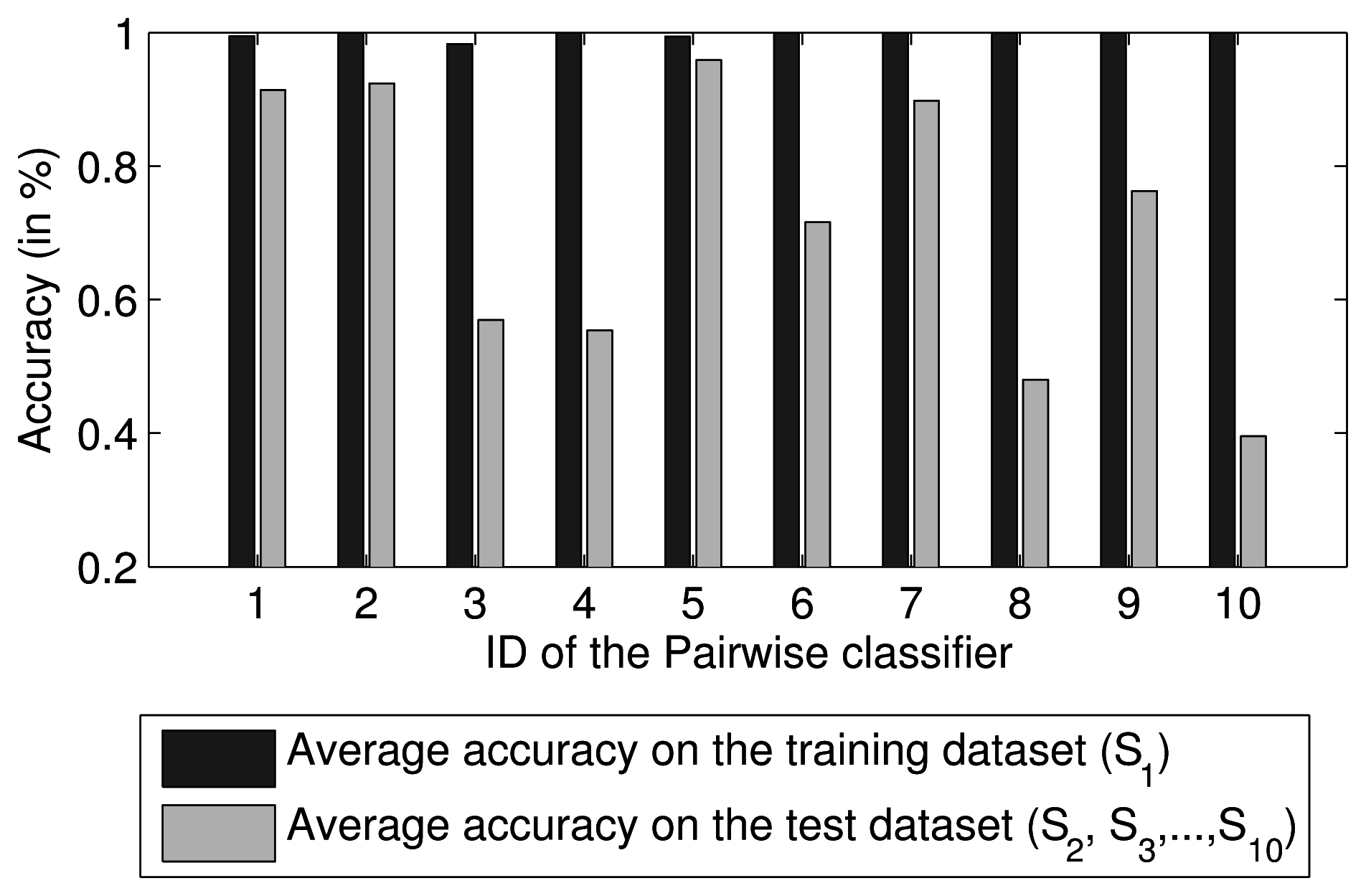
Because two-class problems are much easier to solve than multi-class problems, many researchers have proposed the use of a combination of pairwise comparisons for multi-class classification. The combined approach involves voting or probability estimates [28]. Therefore, a multi-class classifier can be regarded as an ensemble of pairwise classifiers. Because the degree of compactness and overlap in each class region of the feature space is different, the separability between each pair of two classes is also different. Thus, the performance of each pairwise classifier differs. For example, for ten SVM pairwise classifiers trained using the first dataset, S1, collected by Vergara et al. [18], their mean predictive accuracies on S1 and the other datasets are shown in Figure 1. A weighted ensemble of all pairwise classifiers based on their performance should achieve better predictive performance than that of any individual classifier. Thus, a two-dimensional ensemble strategy is proposed in this paper.
3.1. Our Approach
In this section, a two-dimensional (2D) ensemble strategy is proposed. This strategy, which is described in Algorithm 2, comprises two ensemble procedures.
| Algorithm 2 Two-dimensional ensemble strategy. | |
| Require: Datasets St = {(x1, y1), …, (xmt, ymt)}, t = 1, …, T. | |
| 1: | for t = 1, …,T do |
| 2: | Train k(k − 1)/2 pairwise classifiers on St; |
| 3: | Estimate the first-dimensional weight wij for each pairwise classifier using an appropriate technique and normalize the weights; |
| 4: | Combine the k(k − 1)/2 binary classifiers to form the multi-class classifier ft; |
| 5: | Estimate the second-dimensional weight βt of ft using an appropriate technique; |
| 6: | end for |
| 7: | Normalize all second-dimensional weights {β1, …, βT } |
| Ensure: A multi-class classifier ensemble, including T sets of pairwise classifier models, the weights wij for the corresponding multi-class classifiers and the weight βt for each multi-class classifier. | |
In the first ensemble procedure, several multi-class classifiers are obtained by combining the weighted pairwise comparisons. First, k(k − 1)/2 pairwise classifier models are obtained by training a known dataset that contains k classes. Given the observation x and the class label y, we assume that the estimated pairwise class probabilities rij of μij = p(y = i | y = i or j, x) are available. Here, the rij are obtained from the pairwise classifiers. Then, the goal is to construct an ensemble of the pairwise classifiers to estimate , where pi = p(y = i | x), i = 1, …, k. The probability estimation method used in this procedure is that proposed by Wu et al. [28], because this method is used in LibSVM [29], which has been widely applied. The only difference is that the rij used in [28] are replaced with wijrij, where the wij represent the weights for each pairwise classifier, which are referred to as the first dimensional weights in this paper. They are estimated in accordance with the predictive performance of each pairwise classifier. In this approach, the wij represent the prediction accuracy of pairwise comparison on the most recent dataset.
Given T known datasets, T sets of pairwise classifiers can be obtained. Each set of k(k − 1)/2 pairwise classifiers can be combined to form a multi-class classifier in the first ensemble procedure. In the second ensemble procedure, these multi-class classifiers are then combined to form a multi-class ensemble using Algorithm 1, where βt is the prediction accuracy of the t-th multi-class classifier on the most recent dataset, which is referred to as the second-dimensional weight in this paper.
Regarding computational complexity, the time needed for calculating classifier models of the proposed approach equals that of other SVM ensembles, such as that proposed in [18,19]. Because a standard multi-class SVM is a combination of pairwise comparisons, in fact a 1D SVM ensemble also need to calculate the same number of binary classifiers as the proposed approach. The time is incremented only in estimating the first-dimensional weight for each pairwise classifier. As this stage is performed offline, training time is not so dramatic a constraint. Moreover, as most parts of the proposed approach can be easily parallelized or distributed, the time can be reduced when dealing with larger problems.
3.2. Experimental Section 1
In all of our experiments, we trained multi-class SVMs (one-vs.-one strategy) with the RBFkernel using the publicly available LibSVM software. The data used in the experiments was collected by Vergara et al. [18]. Because data for toluene are lacking for nearly one year, we used only the data for the remaining five analytes. To avoid over-fitting and to give a reasonable prediction of the performance, the training dataset and test datasets were collected at different periods of time that did not overlap each other, and the test datasets were not used in any way for training the classifiers. The features in the training and test datasets were scaled appropriately to [−1 1]. The kernel bandwidth parameter γ and the SVM C parameter were chosen using 10-fold cross-validation by performing a grid search in the range [2−10, 2−9, …, 24, 25] and [2−5, 2−4, …, 29, 210], respectively, referring to the parameter setting in [18].
The measurements were combined to form 10 datasets, such that the number of measurements was as uniformly distributed as possible. These datasets were numbered in chronological order as S1, S2,…,S10. The larger the index of the dataset, the later it was collected. Note that 5 months separate the collection of S9 and S10. This gap is extremely significant for this study for two reasons: (1) it enables us to validate our suggested method using an annotated set of measurements that were collected after an elapsed time of five months; and (2) during this period of time, the sensors were exposed to severe contamination, because external interferents could easily and irreversibly become attached to the sensing layer, because the temperature of the sensors was below the operating temperature.
In the experiments, for a given T, we considered that either the values of (Xt, Yt) in St were both known (if t ≤ T) or Xt was known and Yt was unknown (if t > T). Using this data partitioning, we attempted to reproduce real working conditions, in which the system is trained during a limited period of time and is then expected to operate for an extended period of time.
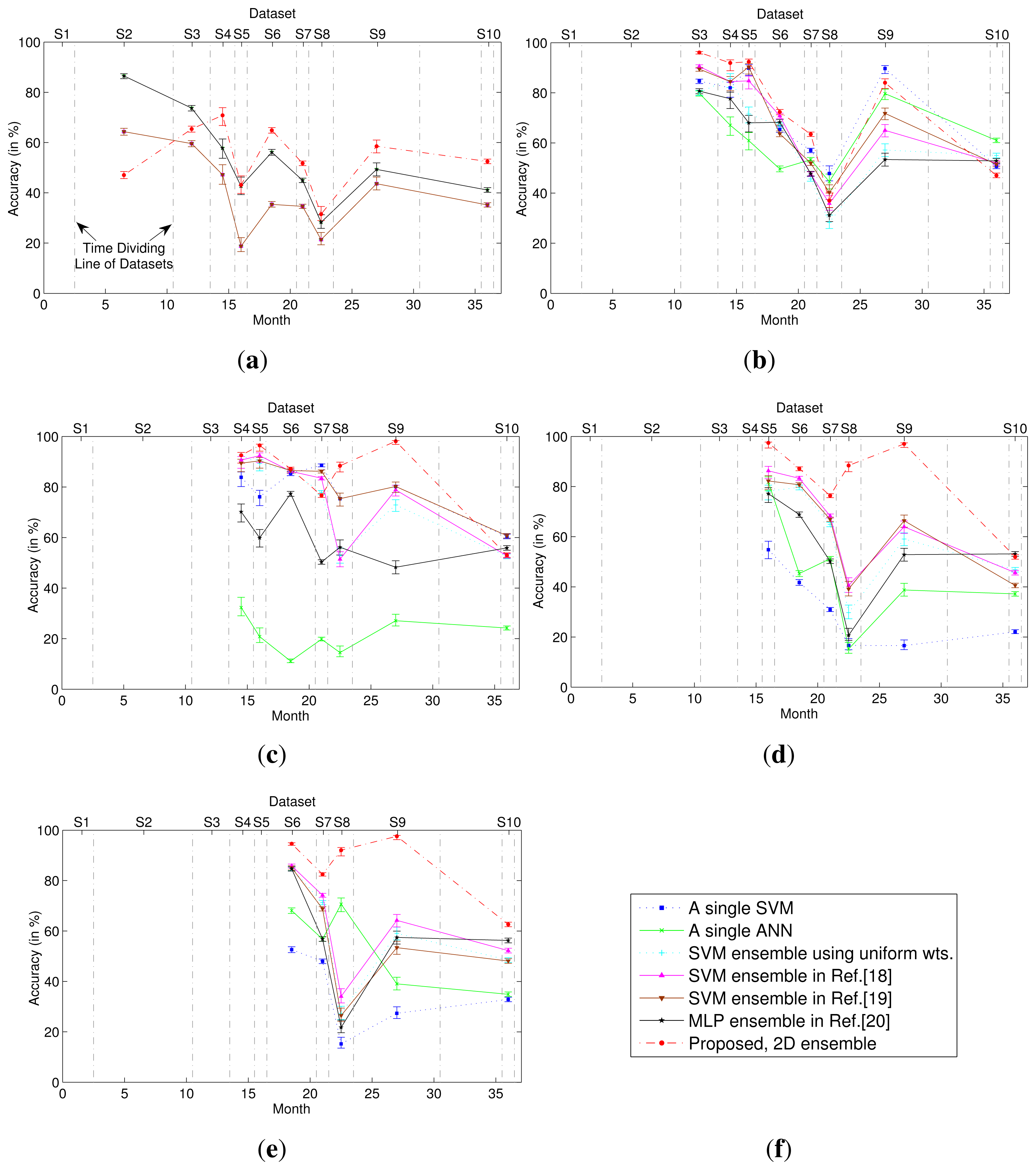
The classification performance of the 2D classifier ensemble was compared with those obtained using different classification methods, including single-model classifiers and 1D classifier ensembles. Figure 2 presents the classification accuracies obtained when T = 1, 2, 3, 4 and 5, where the first Tdatasets were used for training and subsequent datasets were used for testing. For the 1D and 2D classifier ensembles, all weights were estimated on dataset ST. For the single-model classifiers (using a single SVM or ANN), the model was trained on dataset ST. As shown in Figure 2, the 2D classifier ensemble outperformed these single-model classifiers and 1D classifier ensembles when tested on the majority of the unknown datasets, yielding significant improvements in accuracy. Moreover, the larger the number of training datasets, the greater were the advantages of the 2D classifier ensemble.
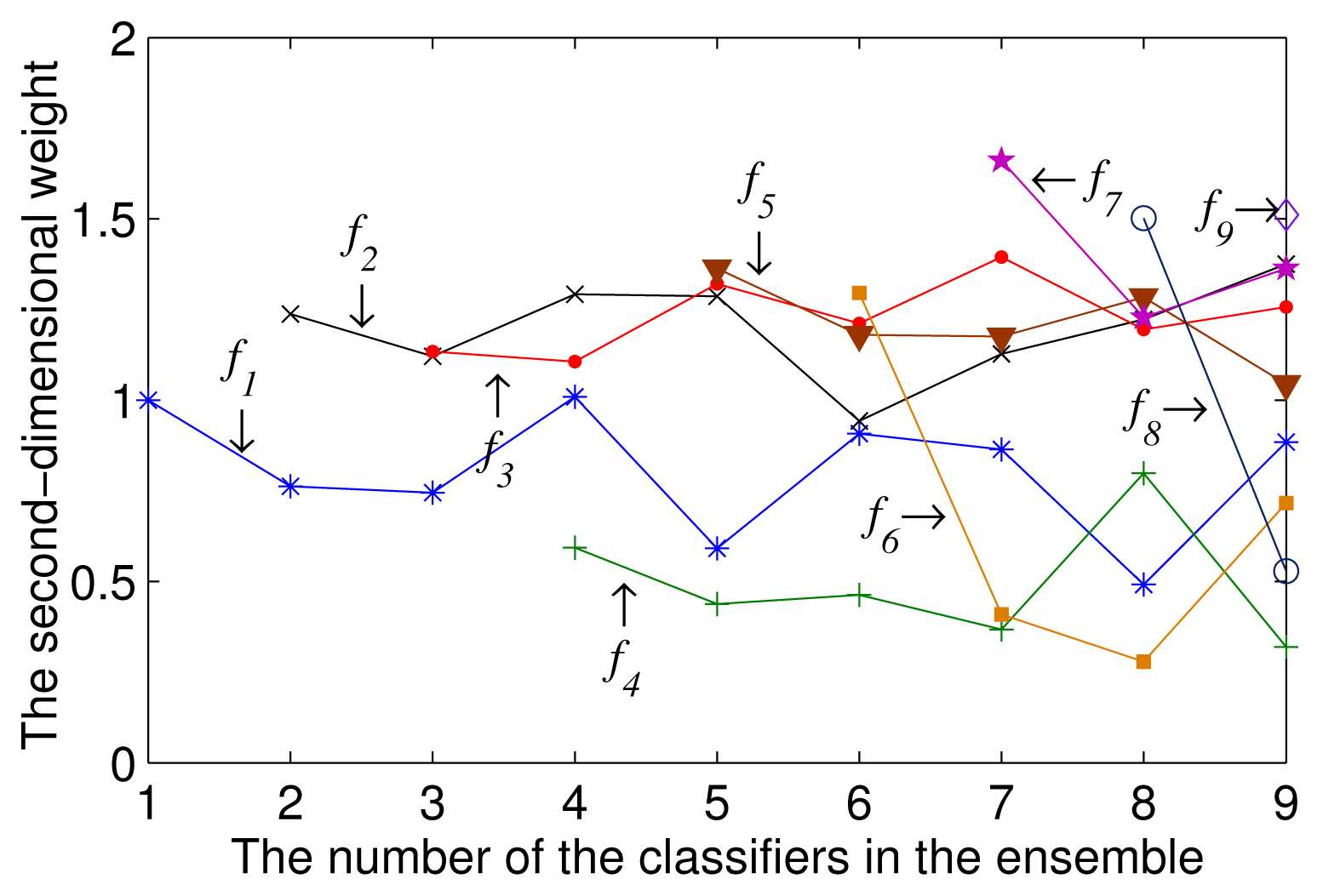
To compare the change of the second-dimensional weight of each multi-class classifier in the ensembles combining varying numbers of multi-class classifiers, we linearly scale all of the weights of the multi-class classifiers, so that their sum is equal to the number of the multi-class classifiers in the ensemble. Figure 3 illustrates how the second-dimensional weight of each multi-class classifier in the ensemble changed with T. As shown in Figure 3, the weight of each classifier fluctuated significantly. This fluctuation caused the ensemble to become excessively sensitive to the training datasets. Moreover, the weights must be re-calculated after the addition of new classifier models to the ensemble.
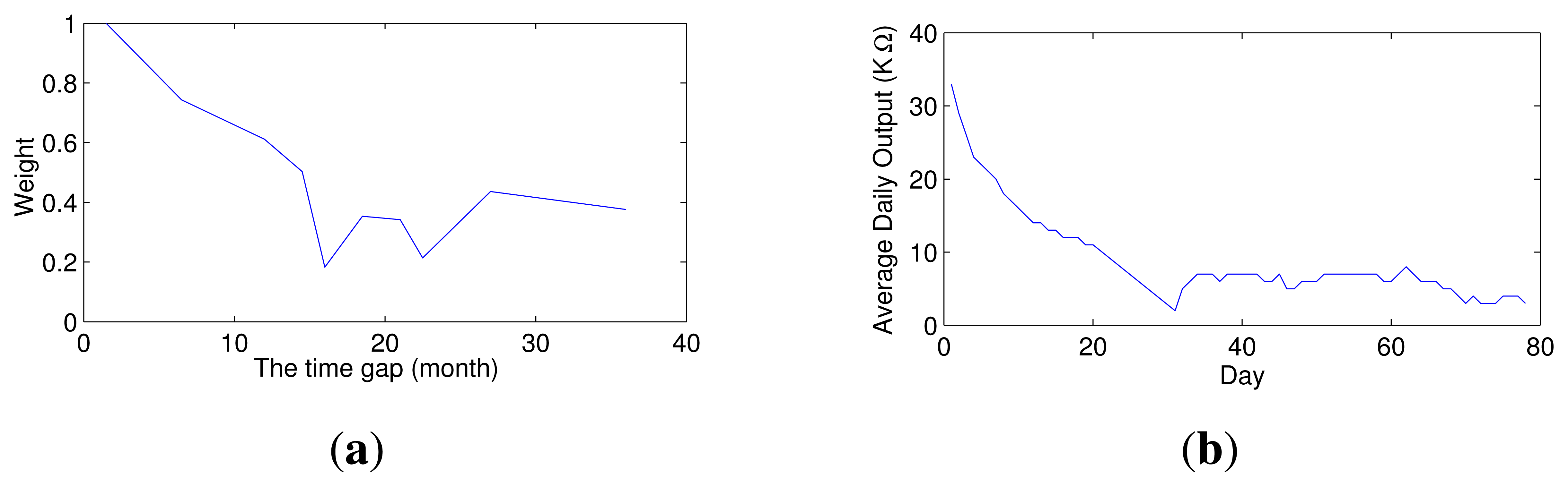
The multi-class classifiers in the ensemble are trained using training datasets collected at different times, whereas their second-dimensional weights are all estimated based on the same dataset, namely the most recent dataset (ST). Thus, the time gap between the training dataset and the dataset that is used to estimate the weight differs for each multi-class classifier. As shown in Figure 4a, this gap significantly affects the weight. If the training dataset of a multi-class classifier is the most recent dataset, then the weight of that classifier is generally the largest among all classifiers in the ensemble; as the gap increases, the weight rapidly decreases. The larger the gap, the higher is the stability of the weight of the multi-class classifier. In other words, the smaller the gap between the training and test datasets, the greater is the accuracy of the multi-class classifier, and as the gap increases, the accuracy initially rapidly decreases and then tends to become stable. This response is similar to that of a gas sensor during the pre-aging process, as illustrated in Figure 4b. A freshly-prepared sensor is highly sensitive, but its sensitivity is unstable. After the pre-aging process, the sensor can maintain a stable performance, but the sensitivity decreases. Thus, gas sensors must be subjected to a pre-aging process to stabilize their performance prior to delivery from the factory. Inspired by the pre-aging process of gas sensors, this paper proposes that the stability of a classifier ensemble can be improved by applying a pre-aging process.
3.3. Pre-Aging Procedure
The schedule of traditional ensembles is as following. At first, if given T known datasets (S1, S2, …, ST), T multi-class classifier models are trained, one on each dataset. All of their weights are estimated using ST, namely the most recent dataset. Generally, the resulting weight of each model changes greatly after the addition of new models to the ensemble. This section proposes two methods of pre-aging a classifier ensemble to keep the weights of original models stable.
3.3.1. The First Pre-Aging Method
This method is based entirely on the pre-aging procedure for gas sensors. At first, a number of classifier models are trained using sets of data. Then their first- and second-dimensional weights are estimated using a more recent dataset in order to pre-age the ensemble. For example, if given T known datasets, the first T − 1 datasets (S1, S2, …, ST−1) are used to train T − 1 separate multi-class classifier models. All of their first- and second-dimensional weights are then estimated using ST, namely the more recent dataset than the training datasets. In this method, only a portion of the known datasets are used for training, so the multi-class classifier models are fewer than the corresponding models without pre-aging.
3.3.2. The Second Pre-Aging Method
This method is an improvement of the first one. If a number of classification models are trained respectively using some training datasets, their first- and second-dimensional weights are estimated using a combination of these training datasets. For example, if given T known datasets, T multi-class classifier models are trained, one on each dataset. All of their first- and second-dimensional weights are estimated using a single set combining S1, S2, …, ST. Compared with the first method, this method does not decrease the number of models.
3.4. Experimental Section 2
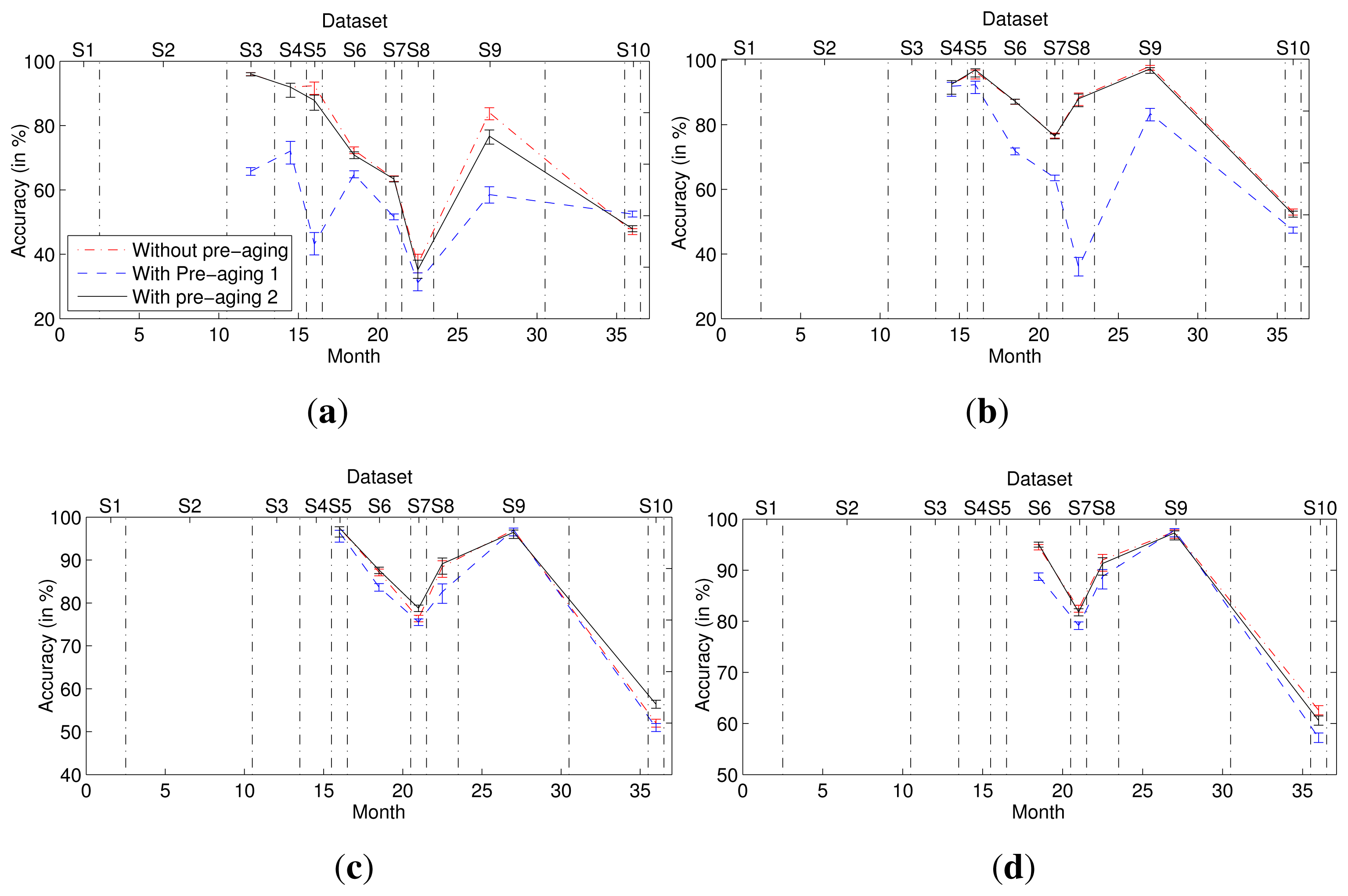
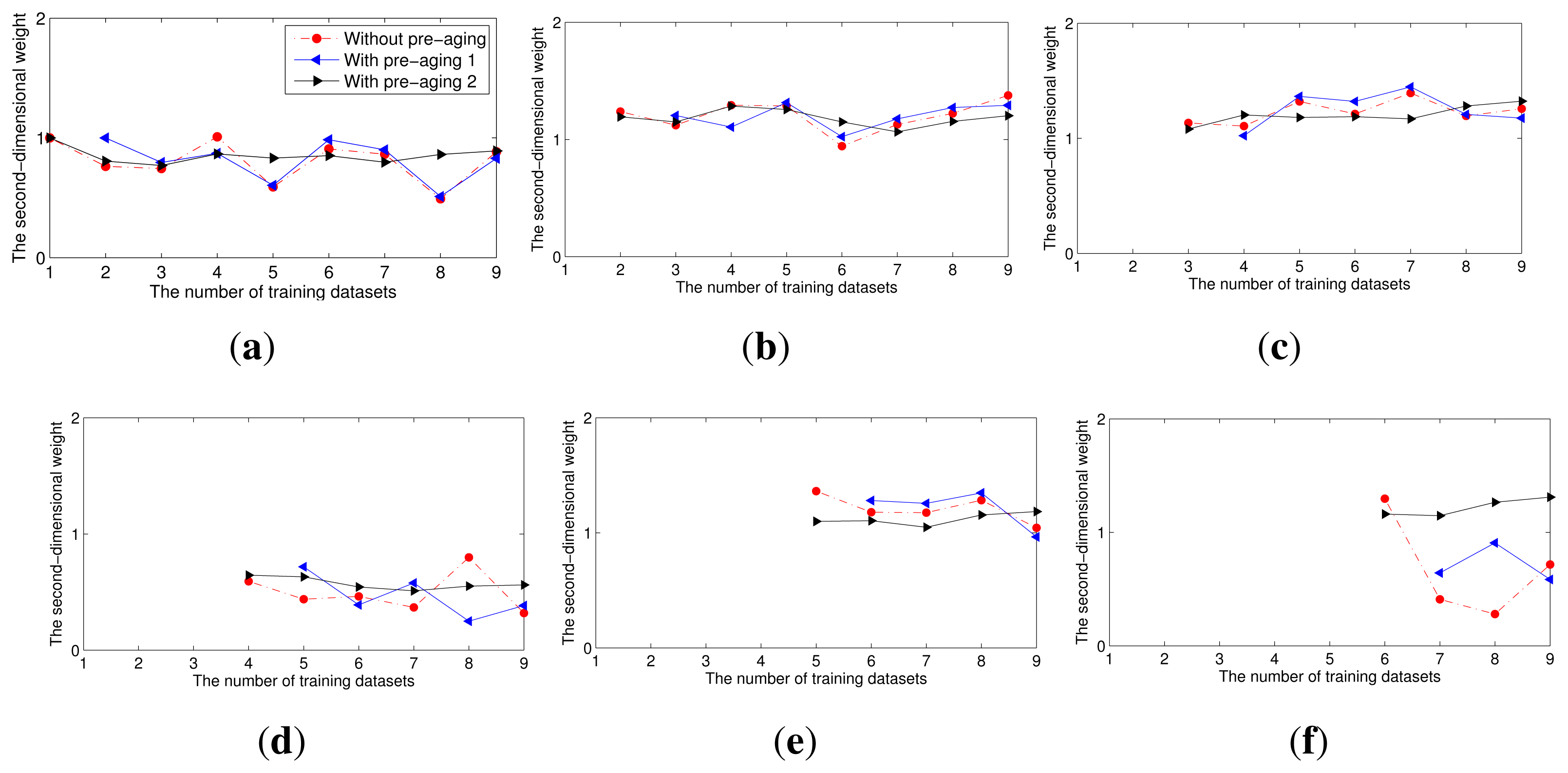
In this experiment, we compared the second-dimensional weights of each multi-class classifier in the ensemble without and with pre-aging (Figure 5) and the corresponding accuracies (Figure 6). To quantify the change of the second-dimensional weights, we calculated the variance of the second-dimensional weights of each multi-class classifier when the ensemble without or with pre-aging contains different numbers of multi-class classifier models. For example, the variance of fi is that of the weights of the multi-class classifier trained using dataset Si when the ensemble contains i, i + 1,…,9 models separately. As shown in Table 1, for each multi-class classifier model, the variance of its second-dimensional weights in the ensembles with the second pre-aging procedure is least. The results indicate that the second-dimensional weight of each multi-class classifier model in the ensemble with the pre-aging process remains fairly static before and after the addition of new classifier models to the ensemble, especially when the second pre-aging method is used. Moreover, the accuracy of the ensemble with the second pre-aging method is slightly superior to the accuracy of the ensemble without pre-aging.
In the first pre-aging method, only part of the known datasets are used for training, and the most recent dataset is used to estimate weights. Different datasets are used to train the classifier and to estimate its weight, thus preventing the weight of one multi-class classifier from substantially exceeding the weights of the other classifiers. However, given the limited availability of known datasets, the number of multi-class classifiers used in the ensemble must be one fewer than that used in a method with no pre-aging, because the most recent dataset, namely ST, is not used to train a classifier. Thus, the accuracy of the ensemble obtained using the first pre-aging method is less than those of the other ensembles. The second-dimensional weight of each multi-class classifier increases in stability when the second pre-aging method is used, and the second pre-aging method also eliminates the deficiency in accuracy of the first method. Thus, the ensemble obtained using the second pre-aging method outperforms that obtained using the first pre-aging method.
4. Conclusions
We introduced a novel two-dimensional classifier ensemble strategy to solve the gas discrimination problem, regardless of the gas concentration. This strategy is appropriate for multi-class classifiers that consist of combinations of pairwise classifiers, such as support vector machines. We compared the performance of this strategy with those of single-model classifiers and 1D classifier ensembles in experiments based on a public dataset that was compiled over a period of three years. The experimental results demonstrated that over extended periods of time, the 2D ensemble outperformed the other methods that were considered.
The weights of the classifiers were found to fluctuate significantly upon the addition of new models to the ensemble. This fluctuation produces an ensemble that is excessively sensitive to the training datasets. Therefore, we proposed a pre-aging process that was inspired by that applied to the sensors to improve the stability of the classifier ensemble. Two methods of pre-aging were proposed in this paper. We demonstrated that the weight of each multi-class classifier model in the ensemble remains fairly static before and after the addition of new classifier models to the ensemble when a pre-aging procedure is applied, especially using the second proposed method. Moreover, the accuracy of the ensemble obtained using the second pre-aging method is slightly superior to that of the ensemble without pre-aging.
Acknowledgements
This work has been supported by the Fundamental Research Funds for the Central Universities (Grant No. DUT14RC(4)03) and the National Natural Science Foundation of China (Grant No. 61131004). The authors thank Vergara et al. for publishing the comprehensive dataset over a period of three years.
Author Contributions
H.L. made substantial contributions to the conception and design of the experiments and wrote the paper. R.C. performed the experiments. H.L. and R.C. analyzed the data. Z.T. contributed analysis tools, provided suggestions and gave final approval of the version to be submitted.
Conflicts of Interest
The authors declare no conflict of interest.
References
- Masson, N.; Piedrahita, R.; Hannigan, M. Approach for quantification of metal oxide type semiconductor gassensors used for ambient air quality monitoring. Sens. Actuators B Chem. 2015, 208, 339–345. [Google Scholar]
- Artursson, T.; Eklöv, T.; Lundström, I.; Mårtensson, P.; Sjöström, M.; Holmberg, M. Drift correction for gas sensors using multivariate methods. J. Chemom. 2000, 14, 711–723. [Google Scholar]
- Padilla, M.; Perera, A.; Montoliu, I.; Chaudry, A.; Persaud, K.; Marco, S. Drift compensation of gas sensor array data by Orthogonal Signal Correction. Chemom. Intell. Lab. Syst. 2010, 100, 28–35. [Google Scholar]
- Ziyatdinov, A.; Marco, S.; Chaudry, A.; Persaud, K.; Caminal, P.; Perera, A. Drift compensation of gas sensor array data by common principal component analysis. Sens. Actuators B Chem. 2010, 146, 460–465. [Google Scholar]
- Distante, C.; Ancona, N.; Siciliano, P. Support vector machines for olfactory signals recognition. Sens. Actuators B Chem. 2003, 88, 30–39. [Google Scholar]
- Ge, H.; Liu, J. Identification of gas mixtures by a distributed support vector machine network and wavelet decomposition from temperature modulated semiconductor gas sensor. Sens. Actuators B Chem. 2006, 117, 408–414. [Google Scholar]
- Lee, D.S.; Jung, H.Y.; Lim, J.W.; Lee, M.; Ban, S.W.; Huh, J.S.; Lee, D.D. Explosive gas recognition system using thick film sensor array and neural network. Sens. Actuators B Chem. 2000, 71, 90–98. [Google Scholar]
- Polikar, R.; Shinar, R.; Udpa, L.; Porter, M.D. Artificial intelligence methods for selection of an optimized sensor array for identification of volatile organic compounds. Sens. Actuators B Chem. 2001, 80, 243–254. [Google Scholar]
- Shi, X.; Wang, L.; Kariuki, N.; Luo, J.; Zhong, C.J.; Lu, S. A multi-module artificial neural network approach to pattern recognition with optimized nanostructured sensor array. Sens. Actuators B Chem. 2006, 117, 65–73. [Google Scholar]
- Szecowka, P.; Szczurek, A.; Licznerski, B. On reliability of neural network sensitivity analysis applied for sensor array optimization. Sens. Actuators B Chem. 2011, 157, 298–303. [Google Scholar]
- Xu, Z.; Shi, X.; Wang, L.; Luo, J.; Zhong, C.J.; Lu, S. Pattern recognition for sensor array signals using fuzzy ARTMAP. Sens. Actuators B Chem. 2009, 141, 458–464. [Google Scholar]
- Gualdrón, O.; Brezmes, J.; Llobet, E.; Amari, A.; Vilanova, X.; Bouchikhi, B.; Correig, X. Variable Selection for Support Vector Machine Based Multisensor Systems. Sens. Actuators B Chem. 2007, 122, 259–268. [Google Scholar]
- Chao, M.; Xin, S.Z.; Min, L.S. Neural network ensembles based on copula methods and Distributed Multiobjective Central Force Optimization algorithm. Eng. Appl. Artif. Intell. 2014, 32, 203–212. [Google Scholar]
- D'Este, C.; Timms, G.; Turnbull, A.; Rahman, A. Ensemble aggregation methods for relocating models of rare events. Eng. Appl. Artif. Intell. 2014, 34, 58–65. [Google Scholar]
- Gao, D.; Chen, M.; Yan, J. Simultaneous estimation of classes and concentrations of odors by an electronic nose using combinative and modular multilayer perceptrons. Sens. Actuators B Chem. 2005, 107, 773–781. [Google Scholar]
- Gao, D.; Chen, W. Simultaneous estimation of odor classes and concentrations using an electronic nose with function approximation model ensembles. Sens. Actuators B Chem. 2007, 120, 584–594. [Google Scholar]
- Shi, M.; Brahim-Belhouari, S.; Bermak, A.; Martinez, D. Committee machine for odor discrimination in gas sensor array. Proceedings of the 11th International Symposium on Olfaction and Electronic Nose (ISOEN), Barcelona, Spain, 13–15 April 2005; pp. 74–76.
- Vergara, A.; Vembu, S.; Ayhan, T.; Ryan, M.A.; Homer, M.L.; Huerta, R. Chemical gas sensor drift compensation using classifier ensembles. Sens. Actuators B Chem. 2012, 166–167, 320–329. [Google Scholar]
- Wang, H.; Fan, W.; Yu, P.S.; Han, J. Mining concept-drifting data streams using ensemble classifiers. Proceedings of the Ninth ACM SIGKDD International Conference on Knowledge Discovery and Data Mining, Washington, DC, USA, 24–27 August 2003; pp. 226–235.
- Amini, A.; Bagheri, M.A.; Montazer, G.A. Improving gas identification accuracy of a temperature-modulated gas sensor using an ensemble of classifiers. Sens. Actuators B Chem. 2013, 187, 241–246. [Google Scholar]
- Muezzinoglu, M.K.; Vergara, A.; Huerta, R.; Rulkov, N.; Rabinovich, M.I.; Selverston, A.; Abarbanel, H.D. Acceleration of chemo-sensory information processing using transient features. Sens. Actuators B Chem. 2009, 137, 507–512. [Google Scholar]
- Rodriguez-Lujan, I.; Fonollosa, J.; Vergara, A.; Homer, M.; Huerta, R. On the calibration of sensor arrays for pattern recognition using the minimal number of experiments. Chemom. Intell. Lab. Syst. 2014, 130, 123–134. [Google Scholar]
- Tang, L.; Peng, S.; Bi, Y.; Shan, P.; Hu, X. A New Method Combining LDA and PLS for Dimension Reduction. PLoS ONE 2014, 9. [Google Scholar] [CrossRef]
- Wang, X.R.; Lizier, J.T.; Nowotny, T.; Berna, A.Z.; Prokopenko, M.; Trowell, S.C. Feature selection for chemical sensor arrays using mutual information. PLoS ONE 2014, 9. [Google Scholar] [CrossRef]
- Liu, Q.; Li, X.; Ye, M.; Ge, S.S.; Du, X. Drift Compensation for Electronic Nose by Semi-Supervised Domain Adaption. IEEE Sens. J. 2014, 14, 657–665. [Google Scholar]
- Zhang, Q.; Chen, Z. A Distributed Weighted Possibilistic c-Means Algorithm for Clustering Incomplete Big Sensor Data. Int. J. Distrib. Sens. Netw. 2014. [Google Scholar] [CrossRef]
- Liu, H.; Tang, Z. Metal Oxide Gas Sensor Drift Compensation Using a Dynamic Classifier Ensemble Based on Fitting. Sensors 2013, 13, 9160–9173. [Google Scholar]
- Wu, T.F.; Lin, C.J.; Weng, R.C. Probability Estimates for Multi-Class Classification by Pairwise Coupling. J. Mach. Learn. Res. 2004, 5, 975–1005. [Google Scholar]
- Chang, C.C.; Lin, C.J. LIBSVM: A library for support vector machines. ACM Trans. Intell. Syst. Technol. 2011, 2, 27:1–27:27. [Google Scholar]


| Classifier | f1 | f2 | f3 | f4 | f5 | f6 |
|---|---|---|---|---|---|---|
| No pre-aging | 0.0312 | 0.0181 | 0.0104 | 0.0306 | 0.0146 | 0.2048 |
| Pre-aging 1 | 0.1777 | 0.0349 | 0.0298 | 0.0567 | 0.0473 | 0.0390 |
| Pre-aging 2 | 0.0045 | 0.0047 | 0.0062 | 0.0028 | 0.0028 | 0.0063 |
© 2015 by the authors; licensee MDPI, Basel, Switzerland. This article is an open access article distributed under the terms and conditions of the Creative Commons Attribution license ( http://creativecommons.org/licenses/by/4.0/).
Share and Cite
Liu, H.; Chu, R.; Tang, Z. Metal Oxide Gas Sensor Drift Compensation Using a Two-Dimensional Classifier Ensemble. Sensors 2015, 15, 10180-10193. https://doi.org/10.3390/s150510180
Liu H, Chu R, Tang Z. Metal Oxide Gas Sensor Drift Compensation Using a Two-Dimensional Classifier Ensemble. Sensors. 2015; 15(5):10180-10193. https://doi.org/10.3390/s150510180
Chicago/Turabian StyleLiu, Hang, Renzhi Chu, and Zhenan Tang. 2015. "Metal Oxide Gas Sensor Drift Compensation Using a Two-Dimensional Classifier Ensemble" Sensors 15, no. 5: 10180-10193. https://doi.org/10.3390/s150510180