
Congestion Based Mechanism for Route Discovery in a V2I-V2V System Applying Smart Devices and IoT

Abstract
:1. Introduction

| Infrastructure | Vehicles | |
|---|---|---|
| Arterial Management | X | |
| Freeway Management | X | |
| Crash Prevention & Safety | X | |
| Road Weather Management. | X | |
| Roadway Operations & Maintenance | X | |
| Transit Management | X | |
| Traffic Incident Management | X | |
| Emergency Management | X | |
| Traveler Information | X | |
| Collision Avoidance | X | |
| Driver Assistance | X | |
| Collision Notification | X |

2. Related Work
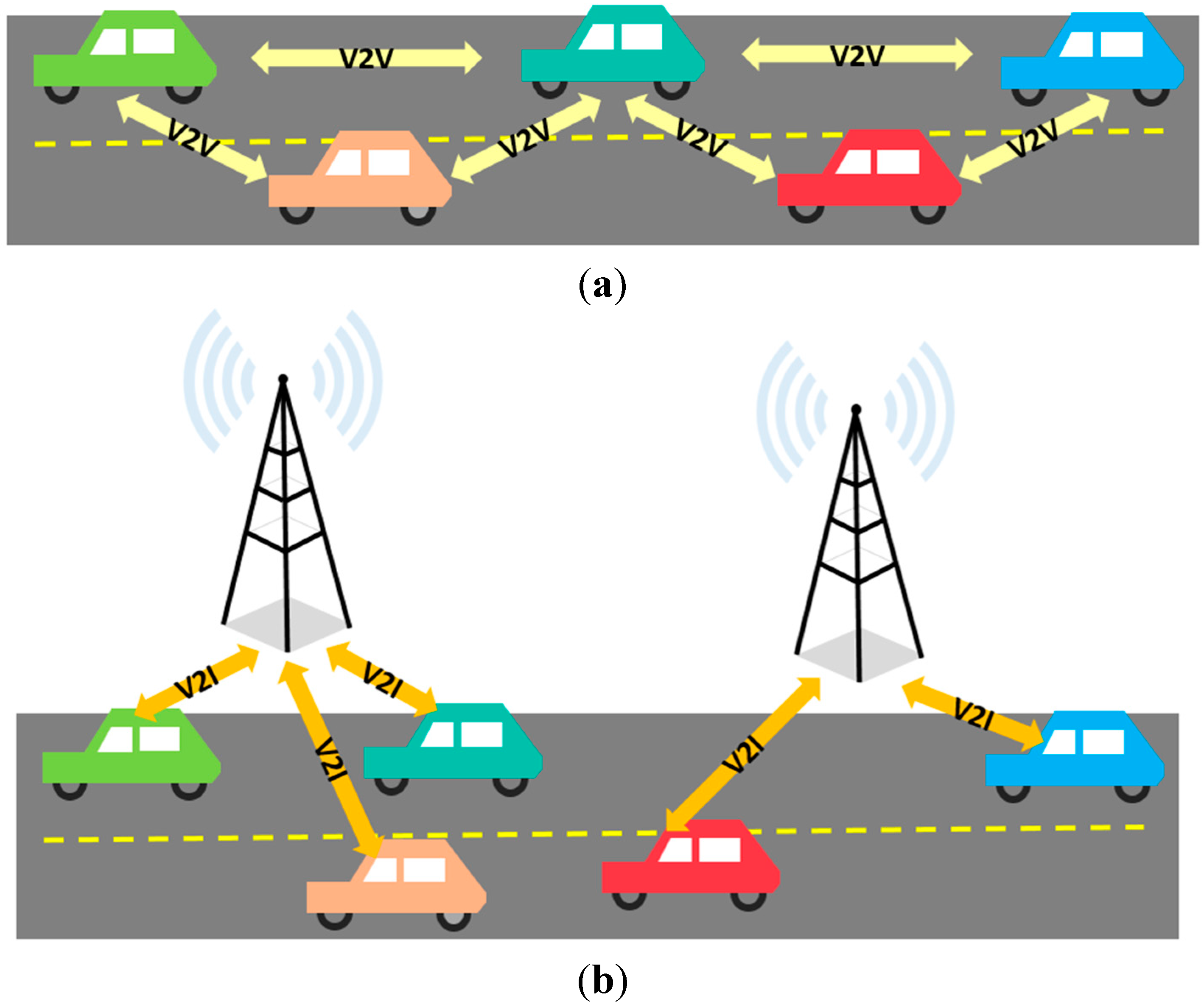
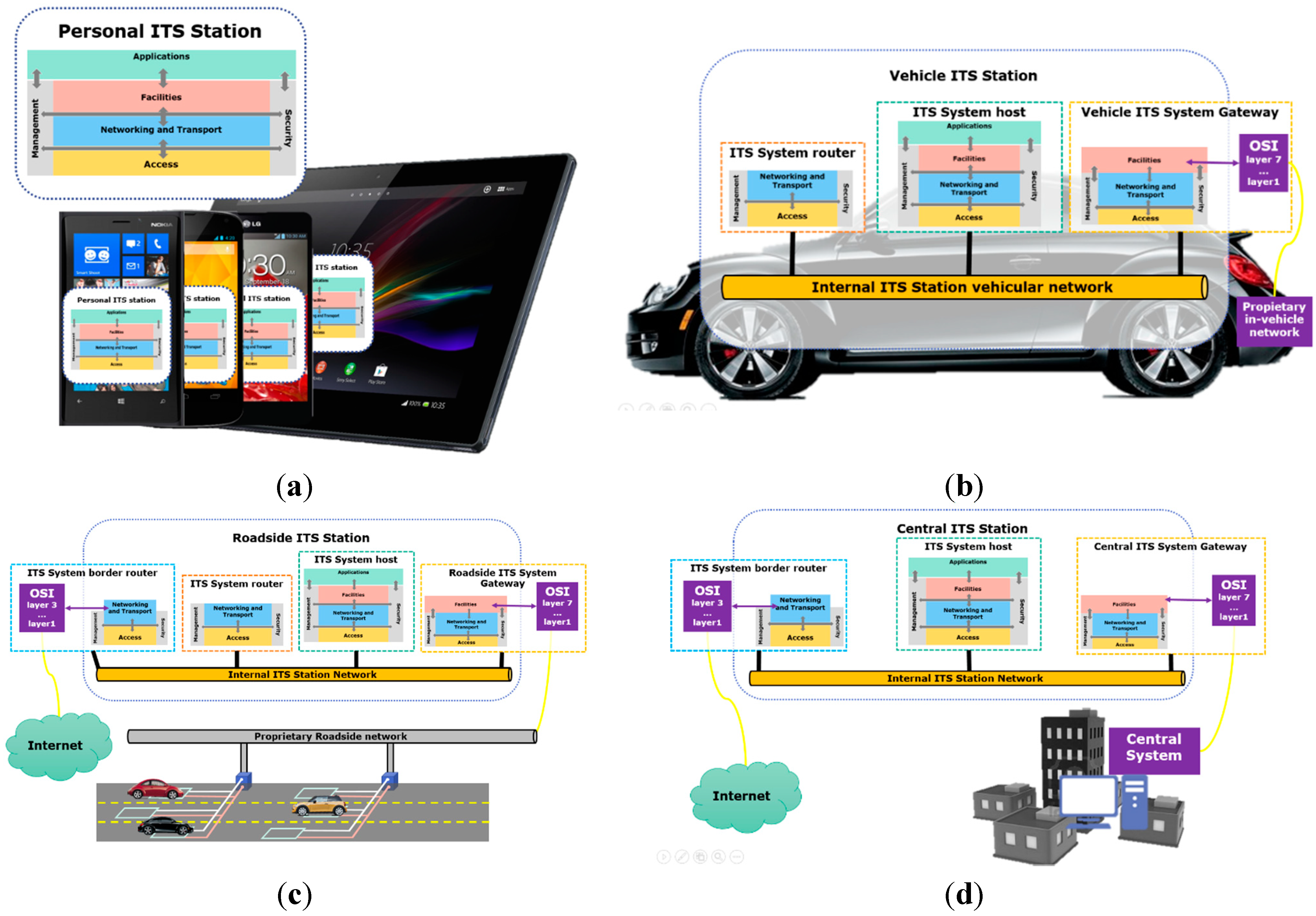
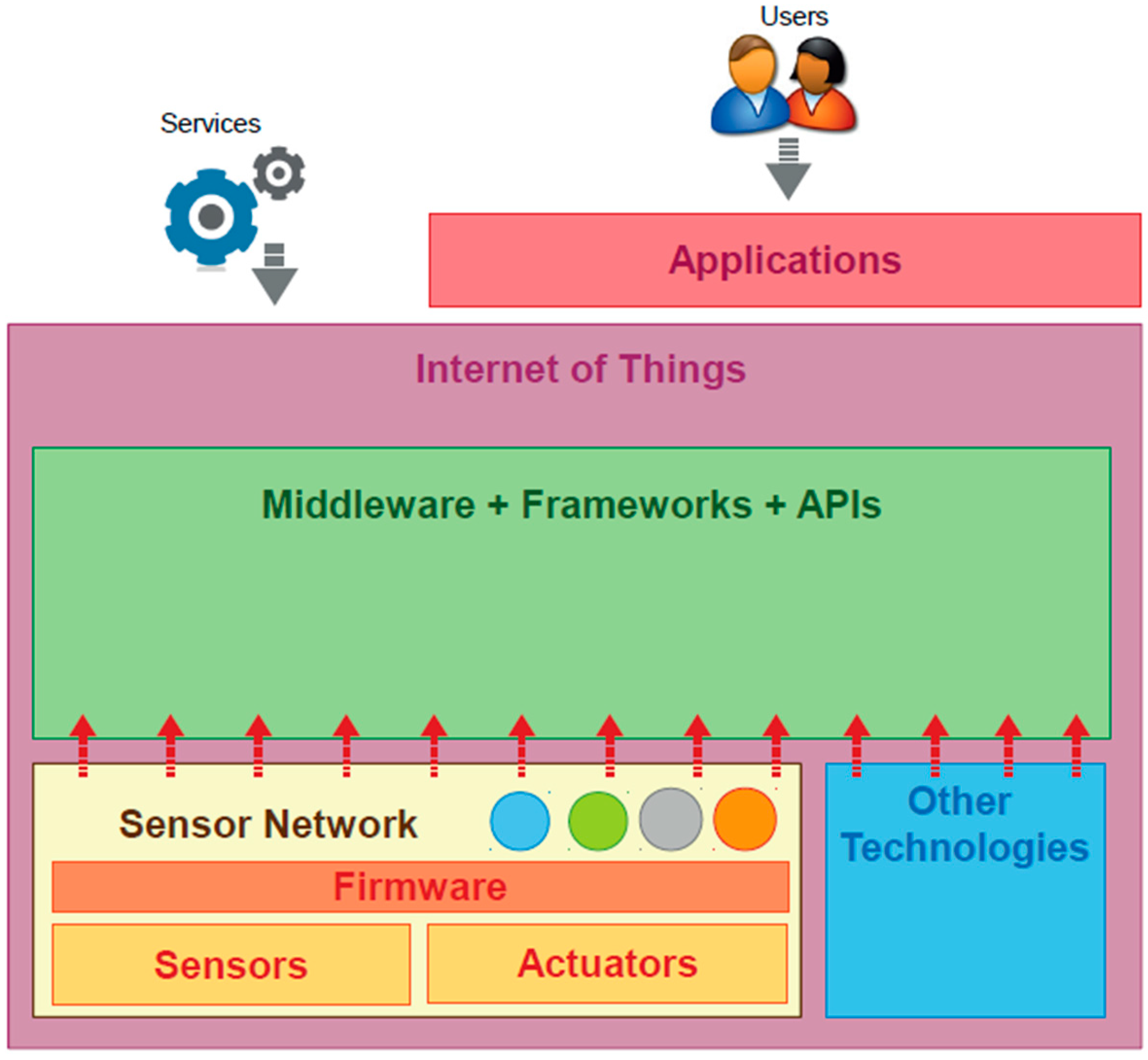
2.1. Technological Background for V2V and V2I Applications


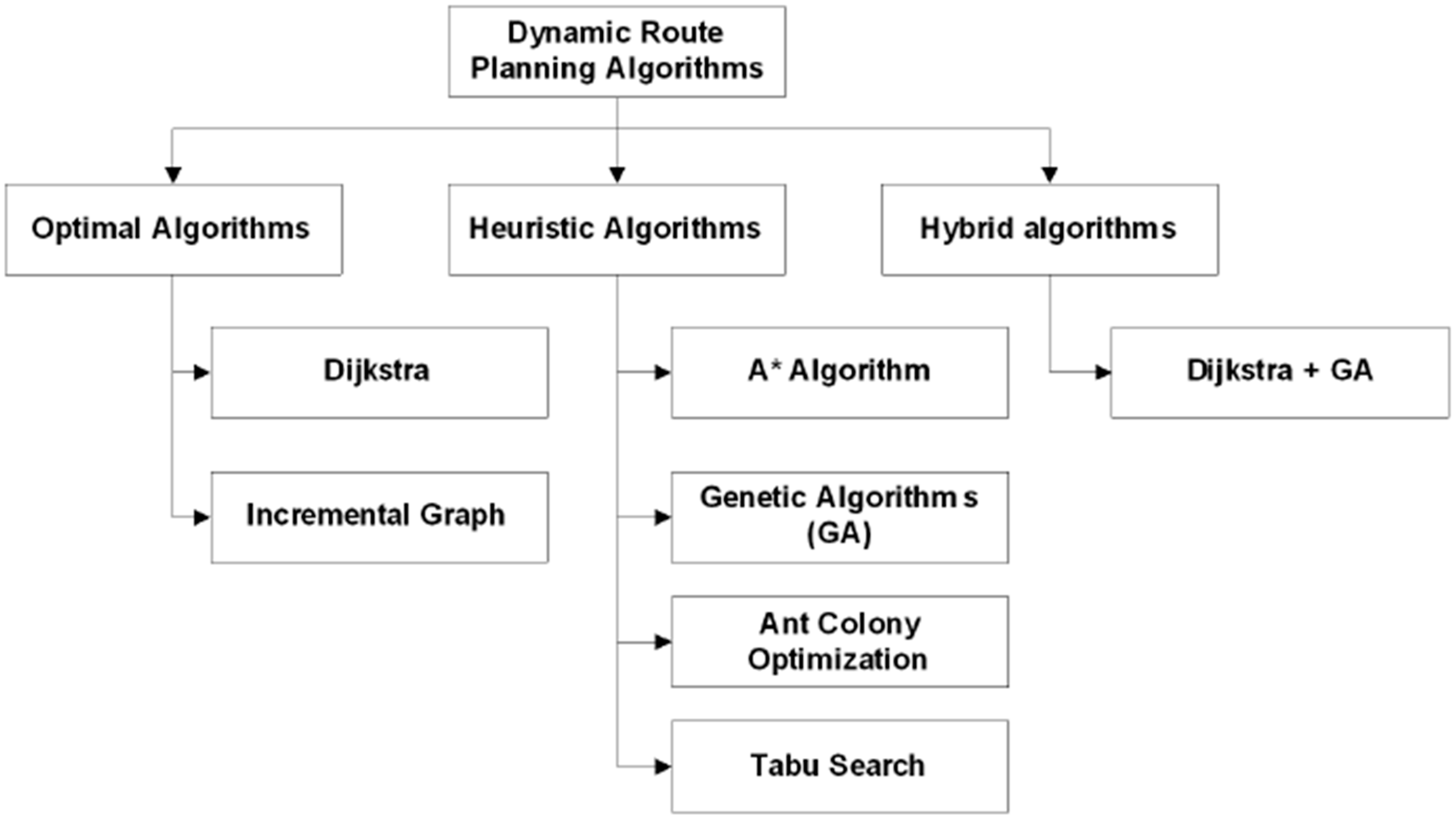
2.2. Existing Dynamic Route Planning Algorithms

3. Optimization Model for Load Balancing in Streets
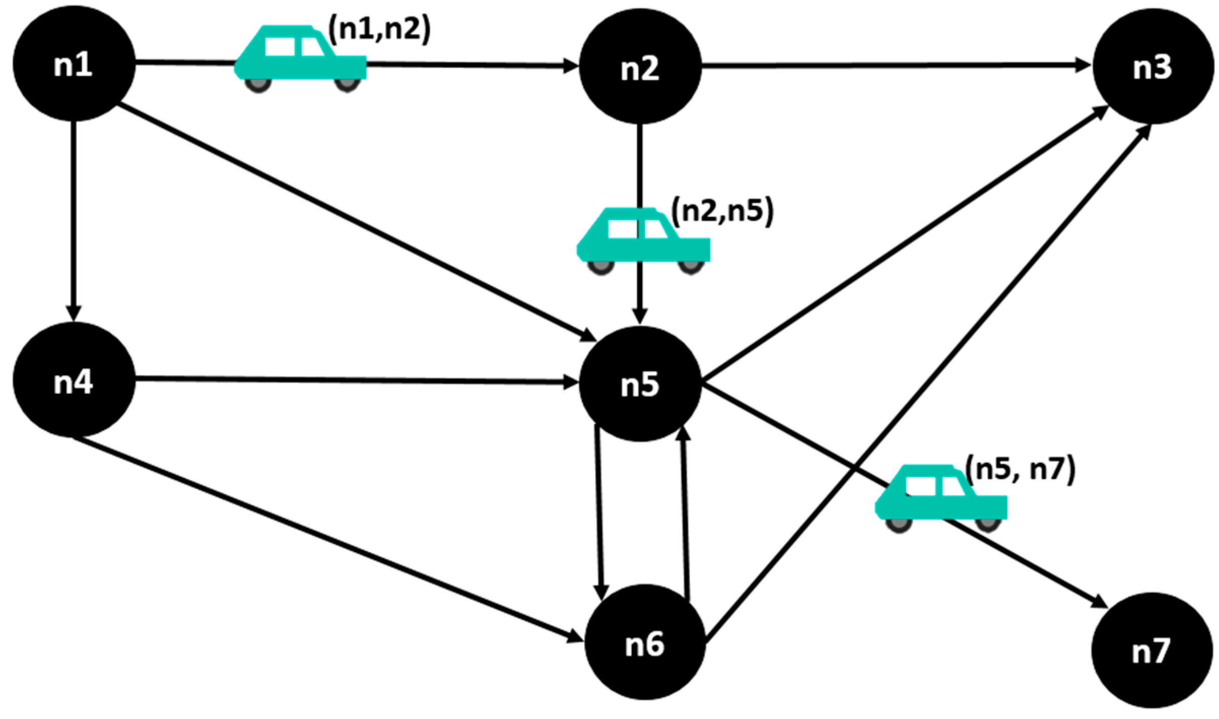
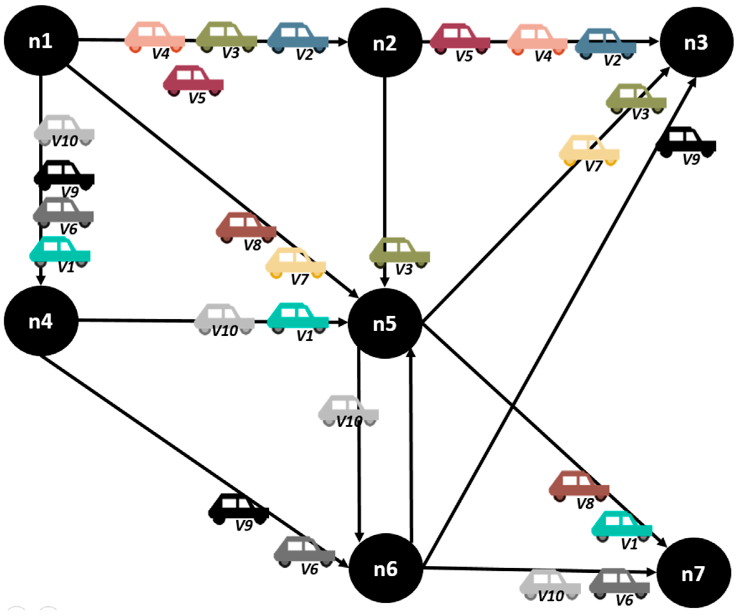
3.1. Vehicular Network Representation

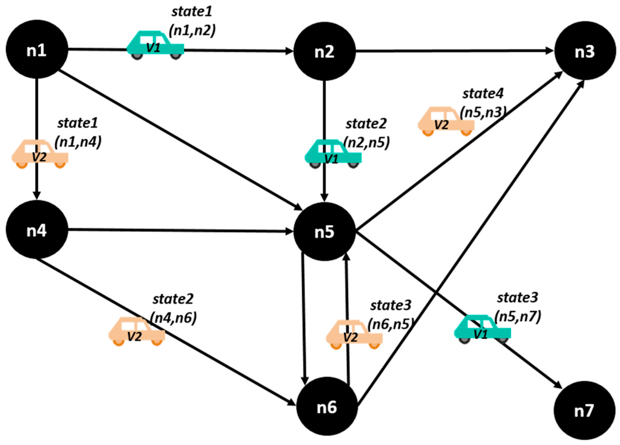
3.2. Definition of Vehicular Congestion in the Optimization Model
3.3. Load Balancing Based on Jain’s Fairness Index
3.4. Model Restrictions
3.4.1. Capacity Restriction
3.4.2. Connectivity Restriction
3.4.3. Flow Restriction in Intermediate Nodes
3.4.4. Destination Node
3.4.5. Conclusions about the Used Model
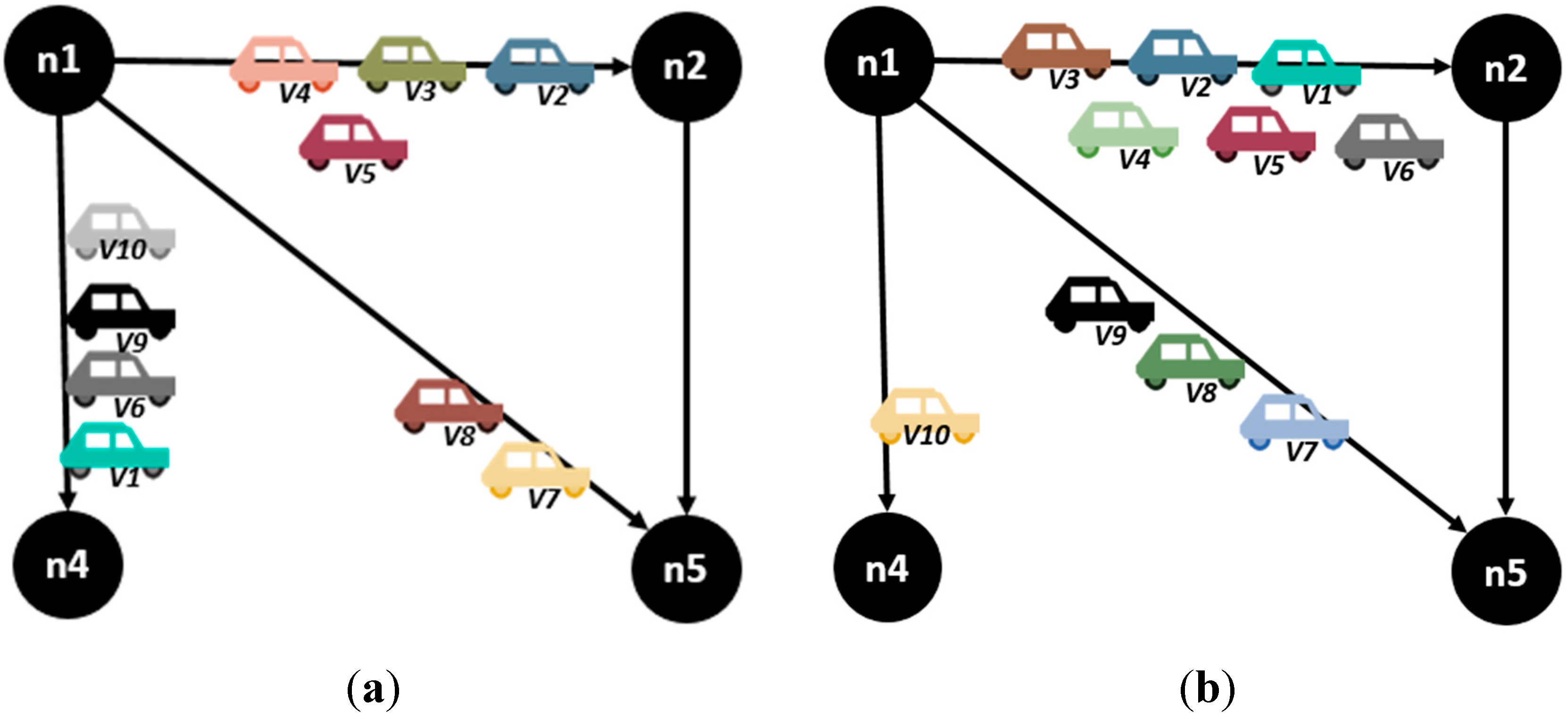
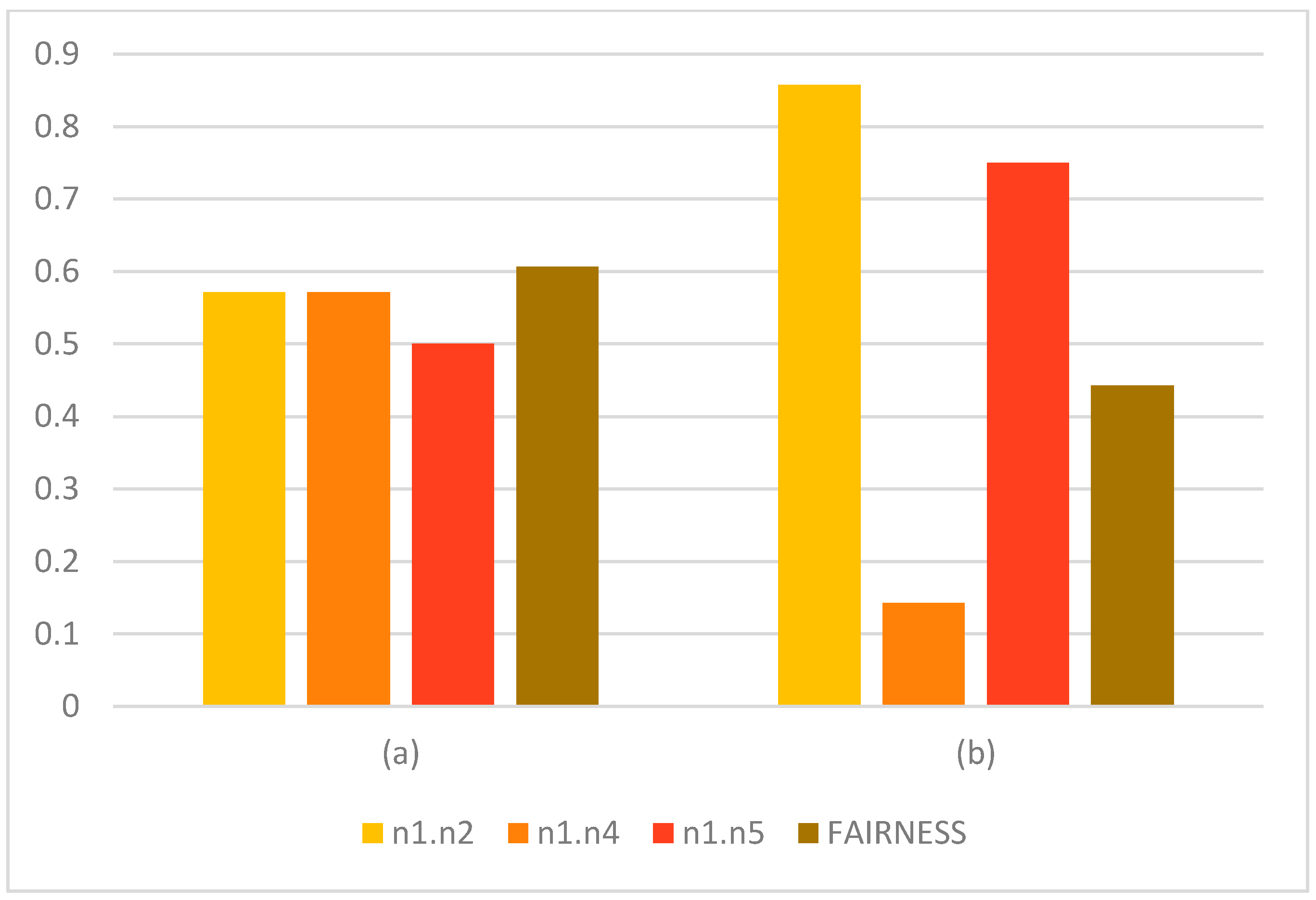
| C(i, j) | U(i, j) (a) | U(i, j) (b) | (a) | (b) | |
|---|---|---|---|---|---|
| n1.n2 | 7 | 4 | 6 | 0.571429 | 0.857143 |
| n1.n4 | 7 | 4 | 1 | 0.571429 | 0.142857 |
| n1.n5 | 4 | 2 | 3 | 0.5 | 0.75 |
| FAIRNESS | 0.606403 | 0.442723 | |||
4. Proposal
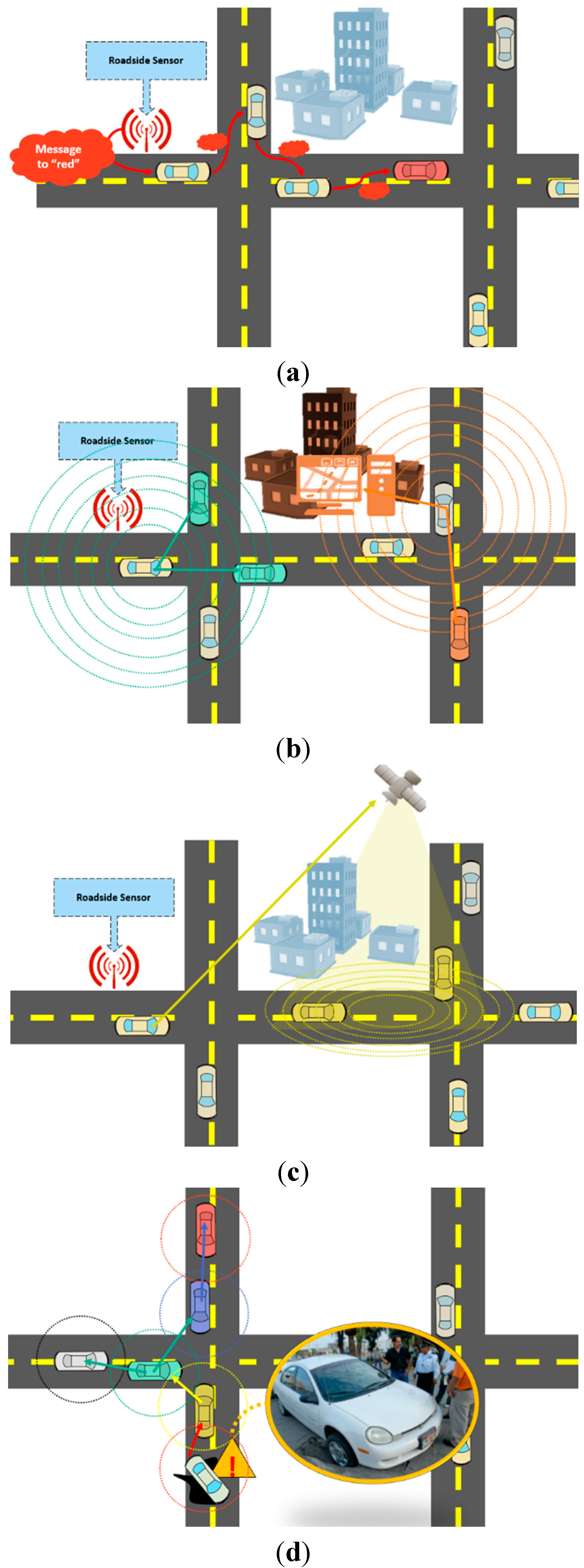
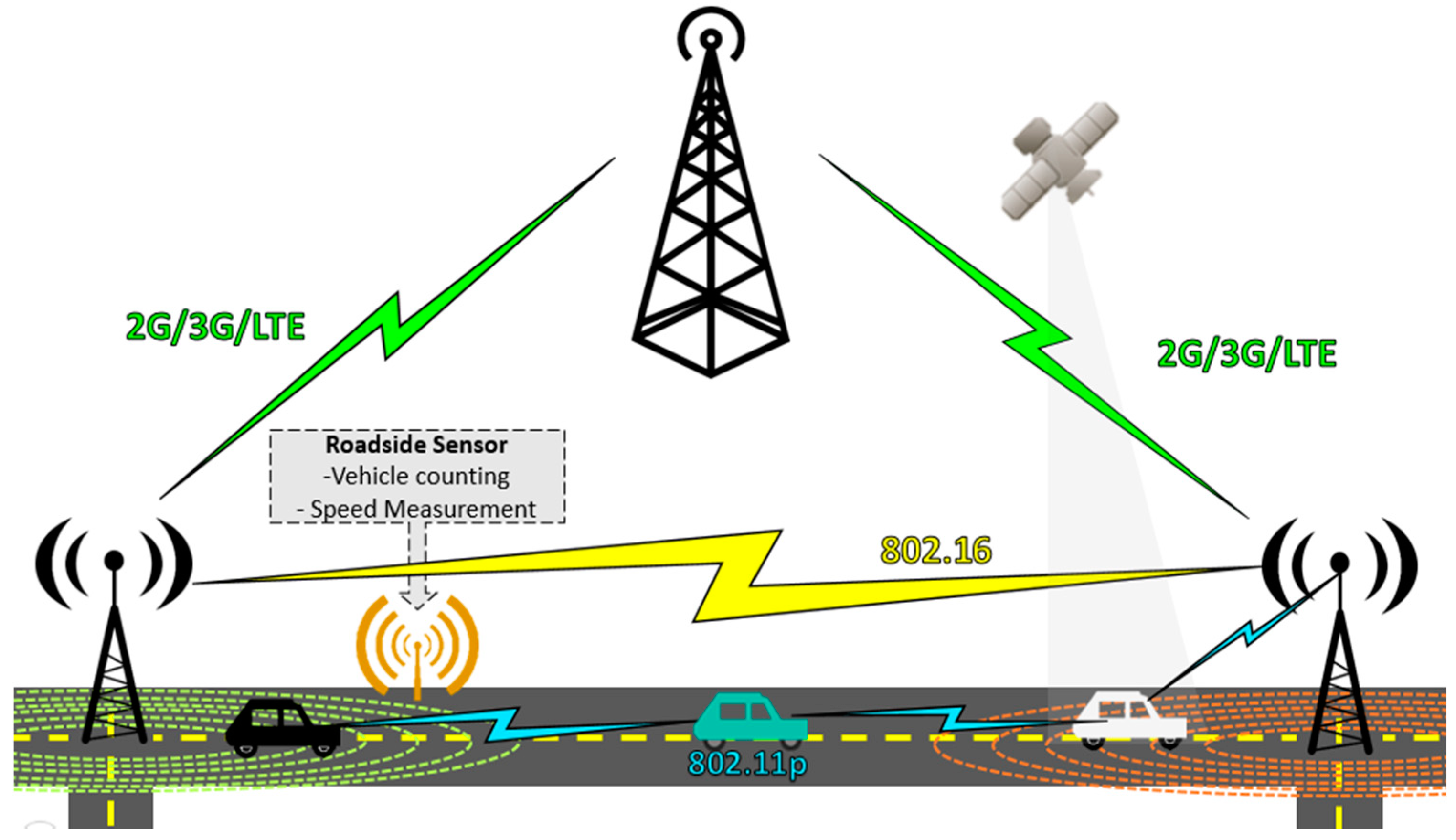
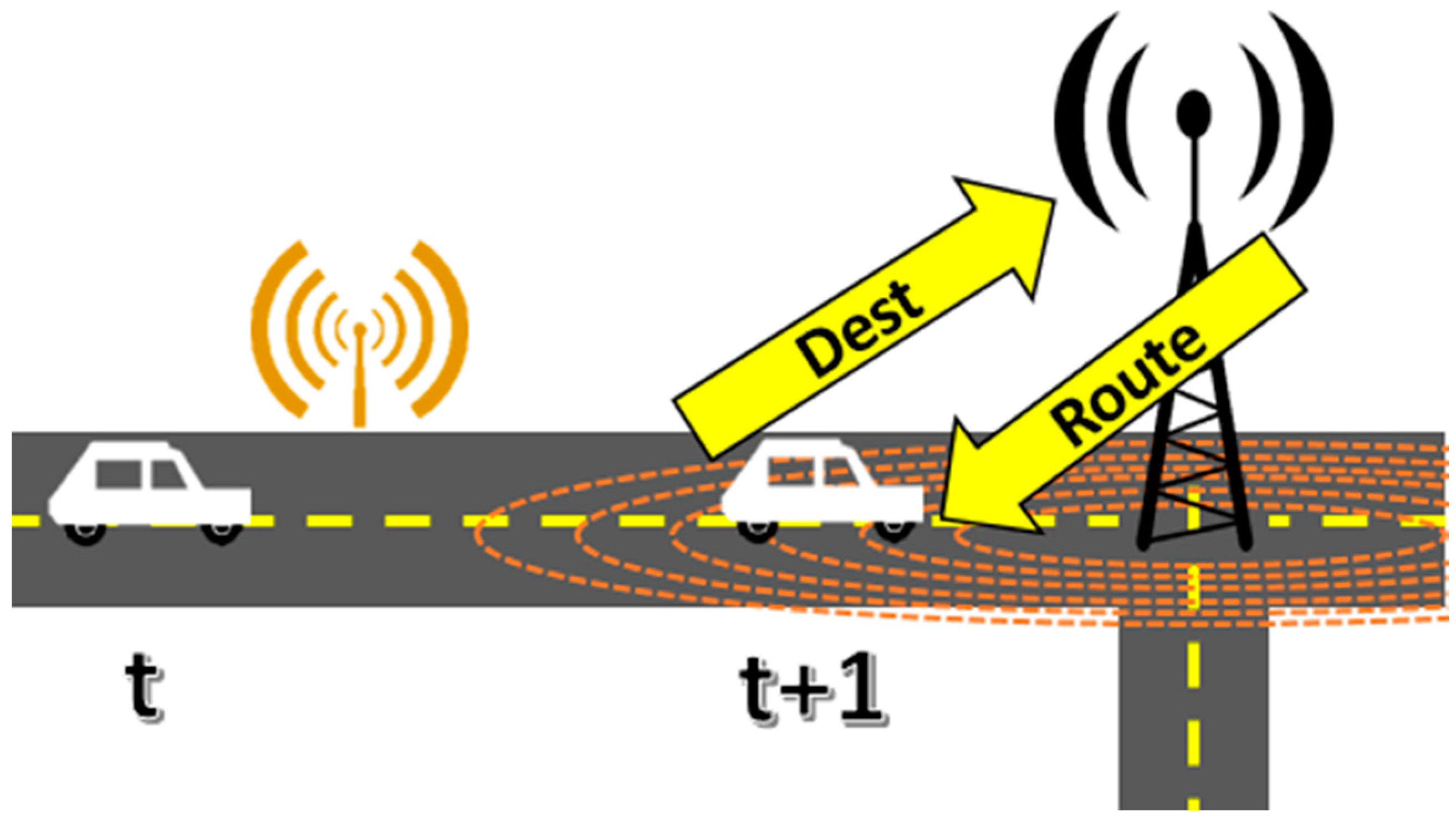
4.1. Communication Technologies and Elements in the Vehicular Network


4.2. Proposed Algorithm
4.2.1. Global Congestion Algorithm (GC)
| Algorithm 1. Global congestion (GC) |
| Require: Vehicle’s destination node Require: All potential paths to : 1: Sort (A to Z) by 2: Path 3: 4: return |
4.2.2. Modified Dijkstra Algorithm (MD)
| Algorithm 2. Modified Dijkstra Route Recalculation (MD) |
Require: Requiring vehicle v Require: Vehicle’s destination node d Require: Actual node actual Require: Adjacent nodes Ad = {k1,…,kn} not empty Require: Adjacency distance matrix d[n] ▷n = number of nodes Require: Un-visited nodes unVisited = { } empty 1: d[actual] = 0 2: add actual to unVisited 3: while Still are nodes in unVisited do 4: Min = get minimal distance node (3) 5: if Min does not exist then 6: return there is no available alternative route 7: else 8: take Min from unVisited 9: for all k in adjacent nodes Ad = {k1,…,kn} do 10: if d[k] > distance(actual,k) + d[Min] then 11: d[k] ← distance(actual,k) + d[Min] 12: end if 13: end for 14: end if 15: end while |
| Algorithm 3. Get minimal distance node |
Require: Un-visited nodes unVisited = {u1,…,un} not empty Require: Actual node actual Require: Adjacency distance matrix d[n] 1: min = NotExists 2: for u in unVisited do 3: if use(actual,u) ≥ capacity(actual,u) AND u is not directly connected to actual then 4: take u from unVisited 5: else 6: if d[u] < d[min] then 7: min ← u 8: end if 9: end if 10: end for 11: return min |
4.2.3. Local-Congestion Based Algorithm (LC)
| Algorithm 4. Local Congestion (LC) |
Require: Requiring vehicle v Require: Actual node actual 1: Node k = Get next node in which congestion is minimal and has space for the vehicle (6) 2: if k exists then 3: return next street (actual,k) 4: else 5: return there is no available route 6: end if |
| Algorithm 5. Get next node |
Require: Adjacent nodes Ad = {k1,…,kn} not empty Require: Actual node actual 1: min = NotExists 2: for k in Ad do 3: if use(actual,k) < capacity(actual,k) AND congestion(actual,k) < congestion(actual,min) 4: min ← k 5: end if 6: end for 7: return min |
4.2.4. Natural Behavior Algorithm
| Algorithm 6. Natural behavior |
Require: Actual node actual Require: Destination node destination 1: Node k = get next node that connects the first available street (7) 2: if k exists then 3: if k = destination then 4: exit network 5: else 6: wait 7: end if 8: else 9: wait 10: end if |
| Algorithm 7. Get first available node |
Require: Actual node actual Require: Adjacent nodes Ad = {k1,…,kn} not empty 1: for k in Ad do 2: if use(actual,k) < capacity(actual,k) then 3: return k 4: end if 5: end for 6: return not Exists |
5. Validation Scenarios
5.1. Scenarios Definition
5.1.1. Control Scenario

5.1.2. Reference Scenario


(a) Street Capacity
- For , approximate distances that provides Google Maps for each street network are taken.
- For , is taken as an average length for all vehicles 3.8 m and 2.4 m of vehicle separation, so that the total is 6.2 m.
(b) Origin/Destination Pairs for Each Vehicle and Approximate Flow
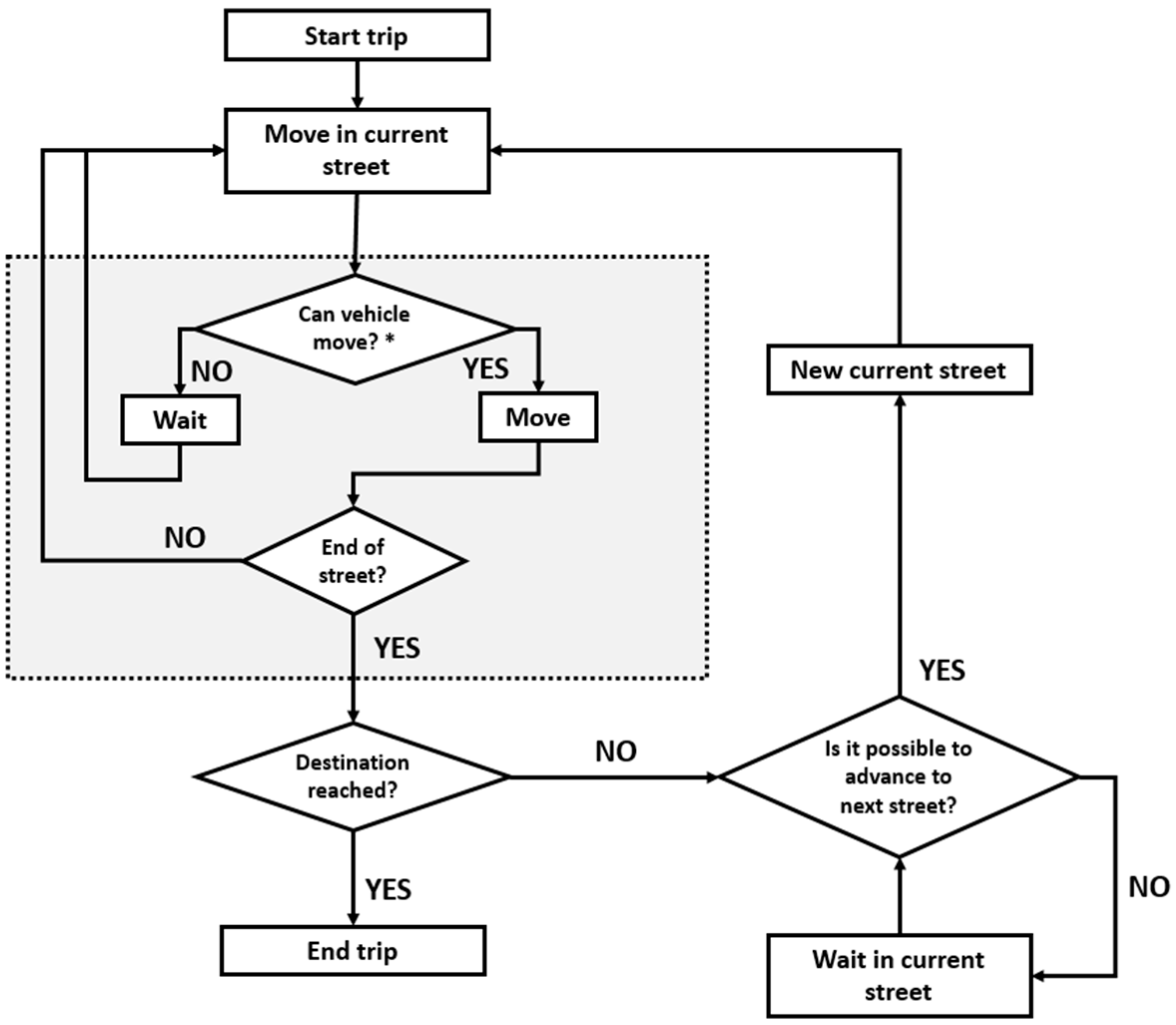
5.2. Simulation Description

5.3. Comparison Metrics
5.3.1. Route Efficiency
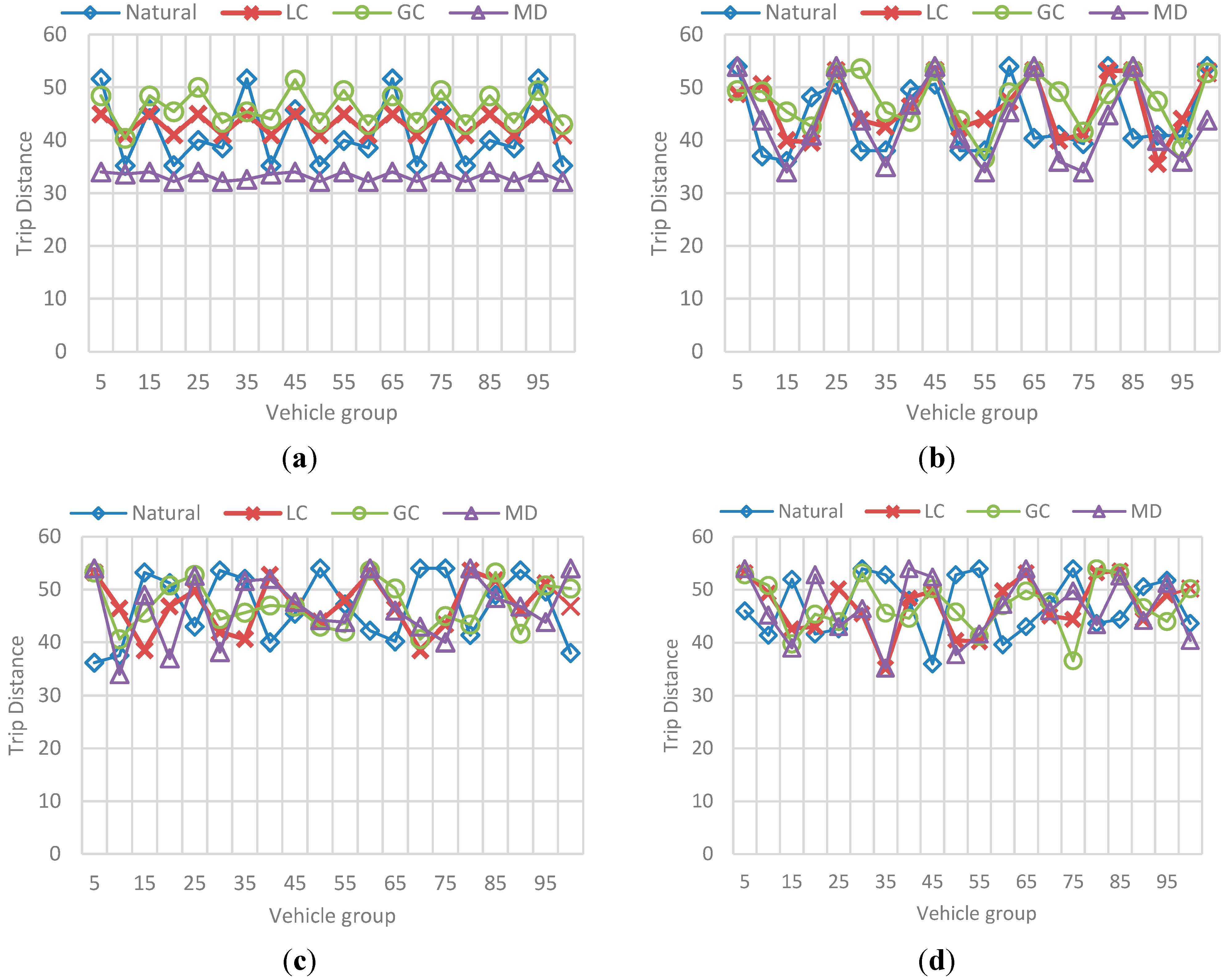
5.3.2. Traveled Distance
5.3.3. Fairness Index
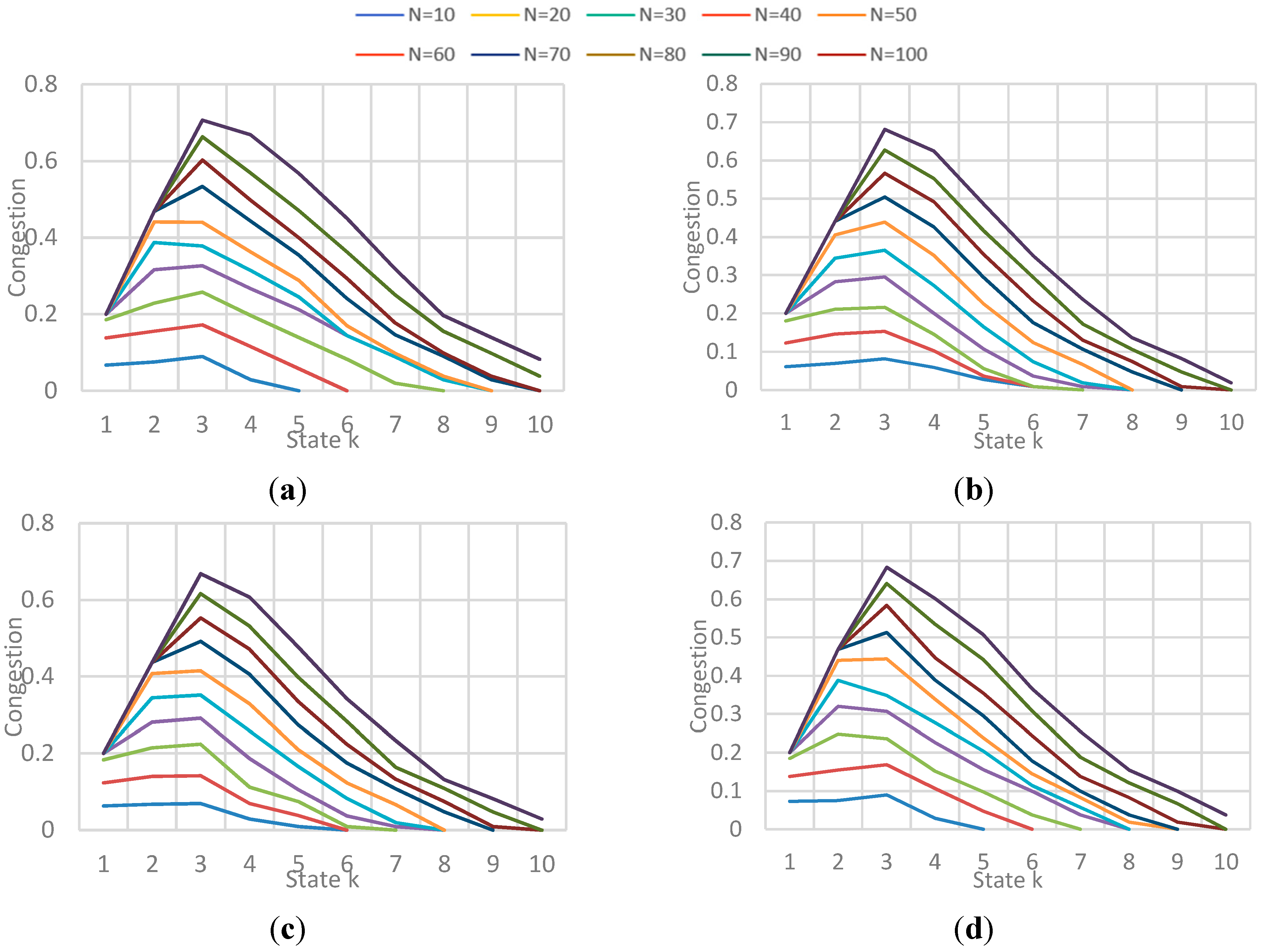
5.3.4. Congestion
6. Obtained Results
6.1. Obtained Results Presentation
6.1.1. General Behavior
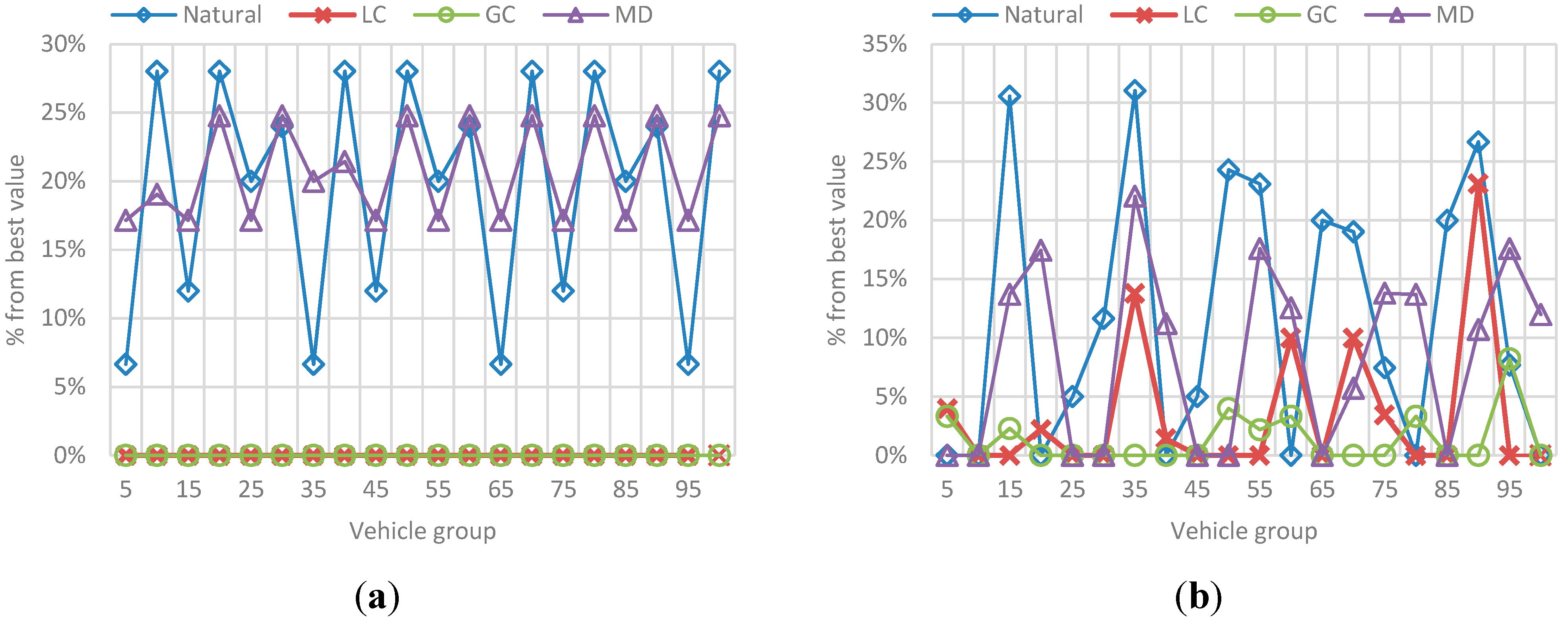
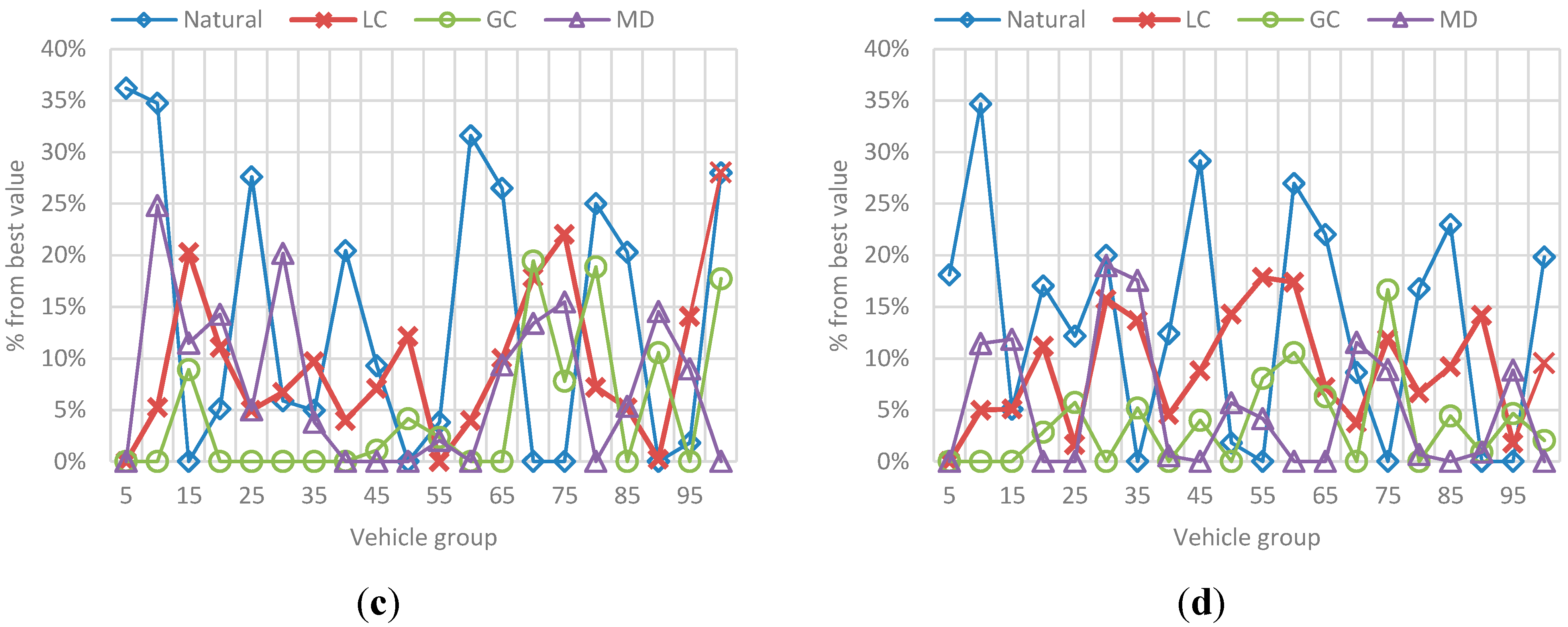
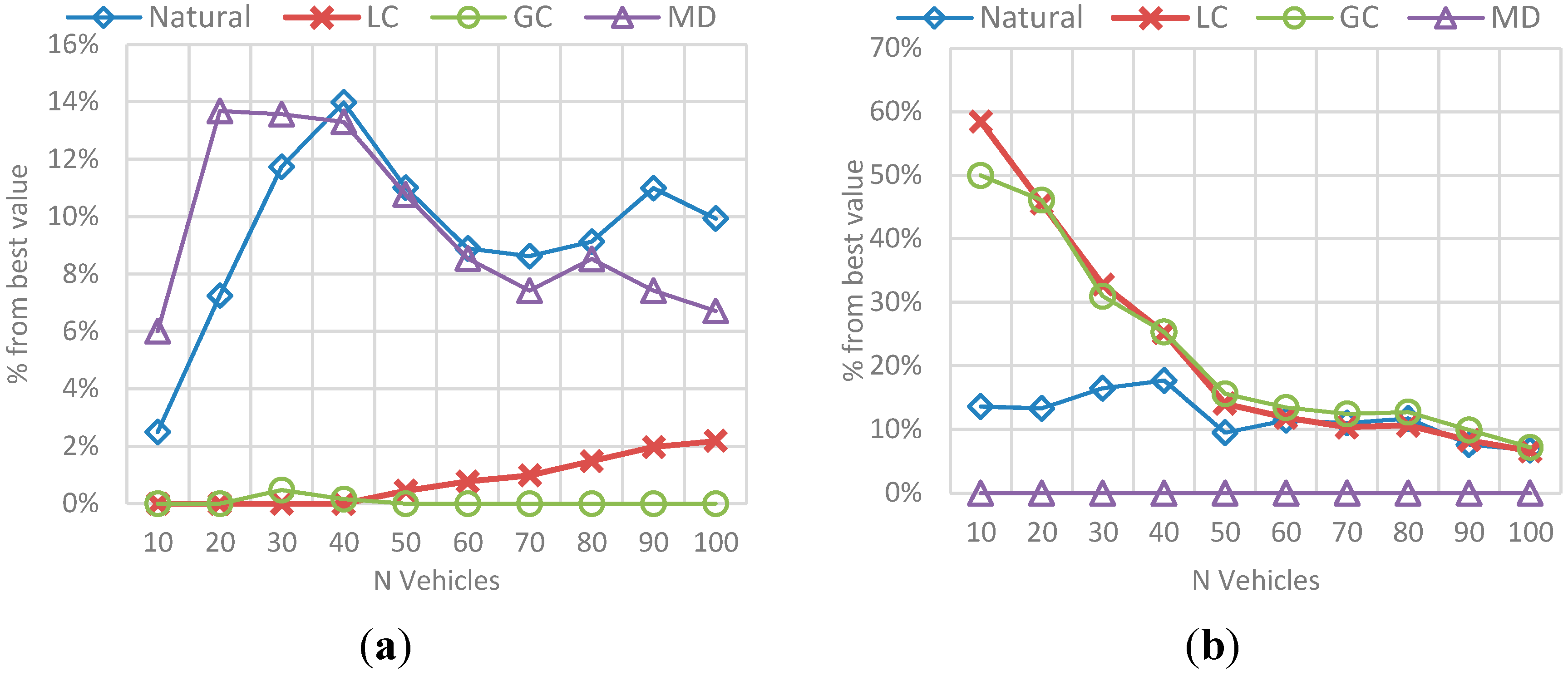
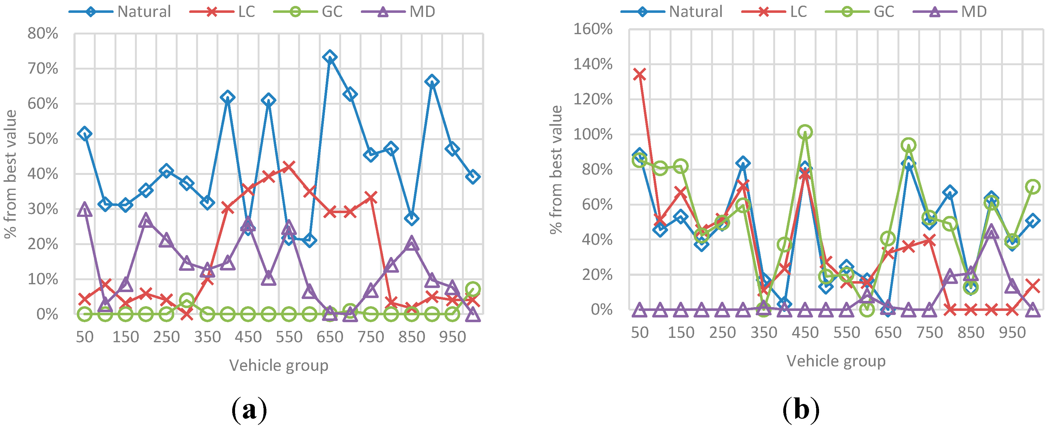
6.1.2. Comparison against the Best Value
6.2. Control Scenario Results
6.2.1. N Vehicles
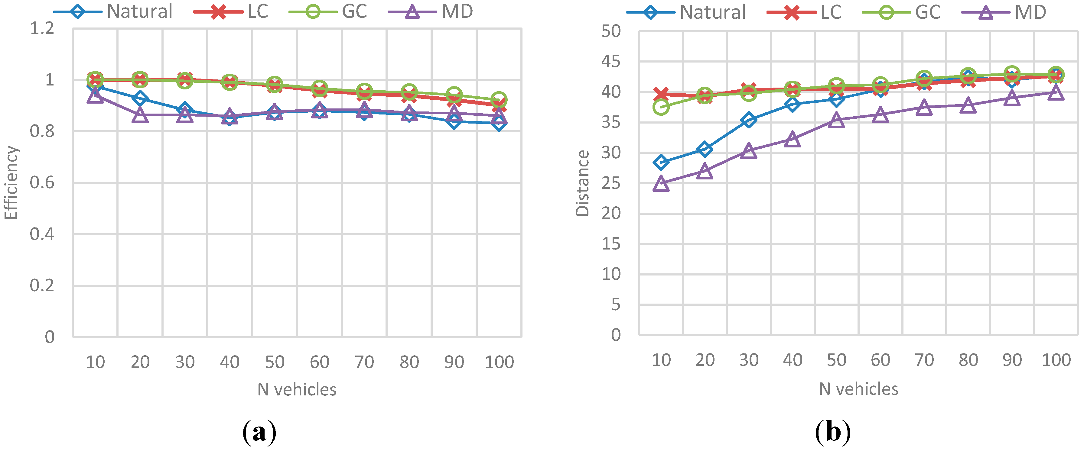
(a) Efficiency and Distance

- -
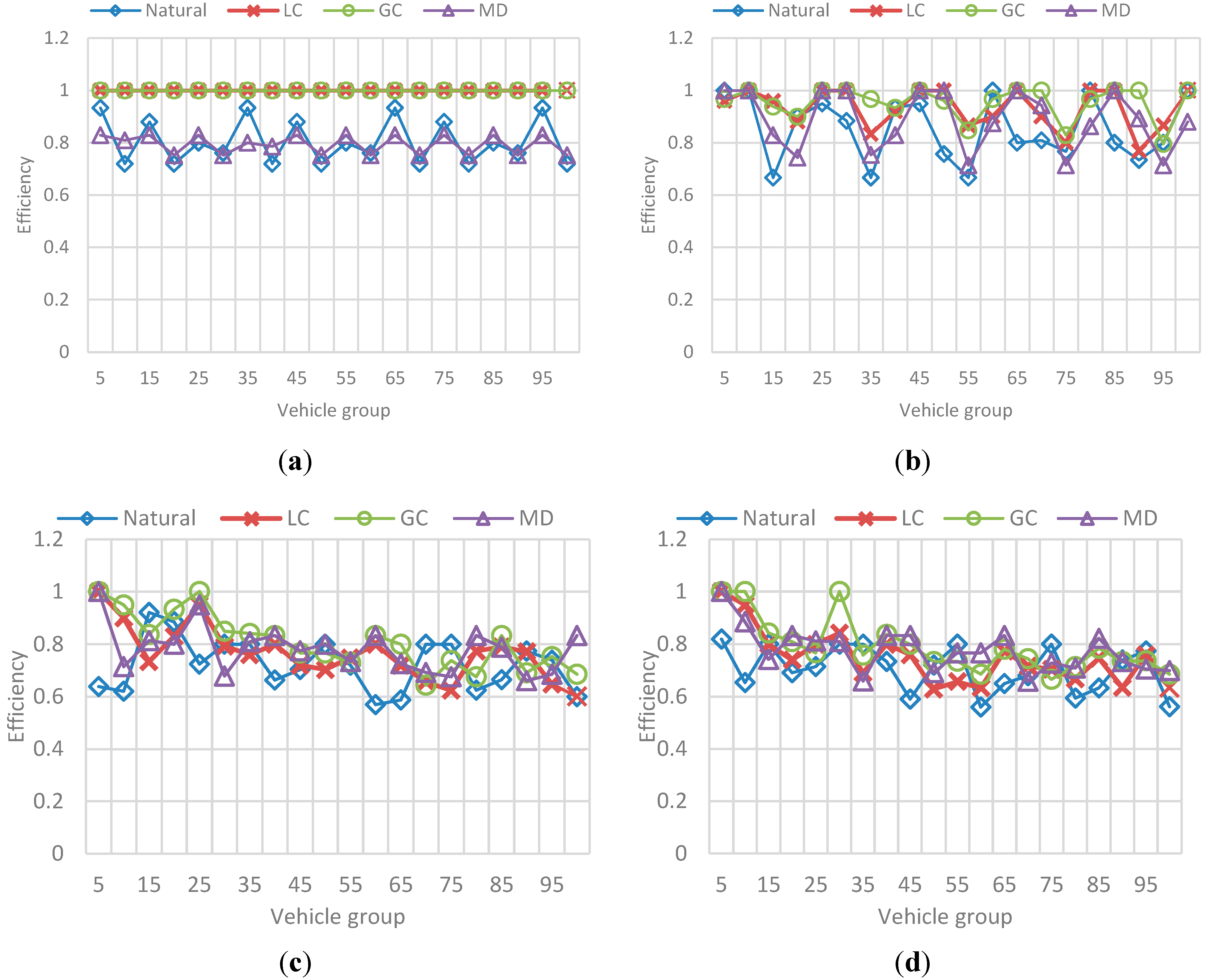
- The route efficiency in all implementations decreases as the set of vehicles in the network is bigger.
- -
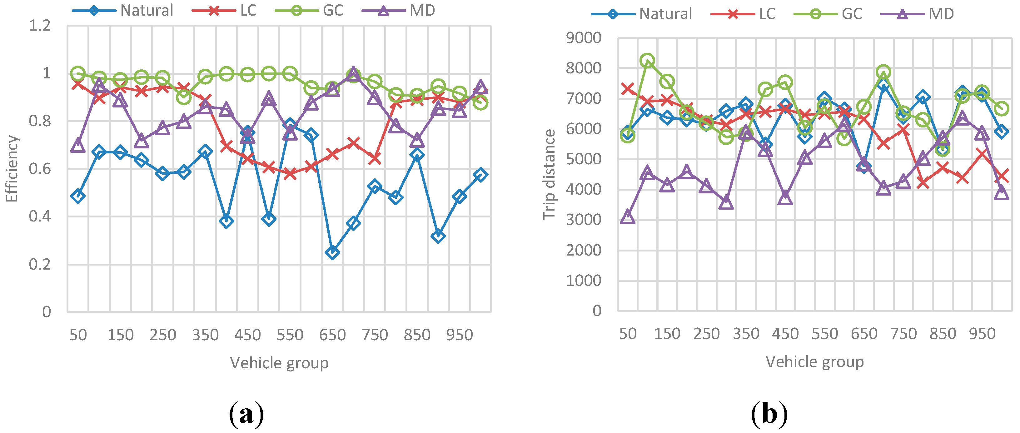
- The trip distance is affected by the amount of vehicles in the network and it increases as the number of vehicles grows, even for the MD solution.
- -
- Even when the efficiency levels are always between 0.8 and 1 and the variability in the results is not very large, GC had a better result with respect to the other implementations, followed by LC.
- -
- On the other hand, that implementation has one of the biggest average trip distance among the vehicles, which means it exists a trade-off between the travelled distance and the route efficiency.
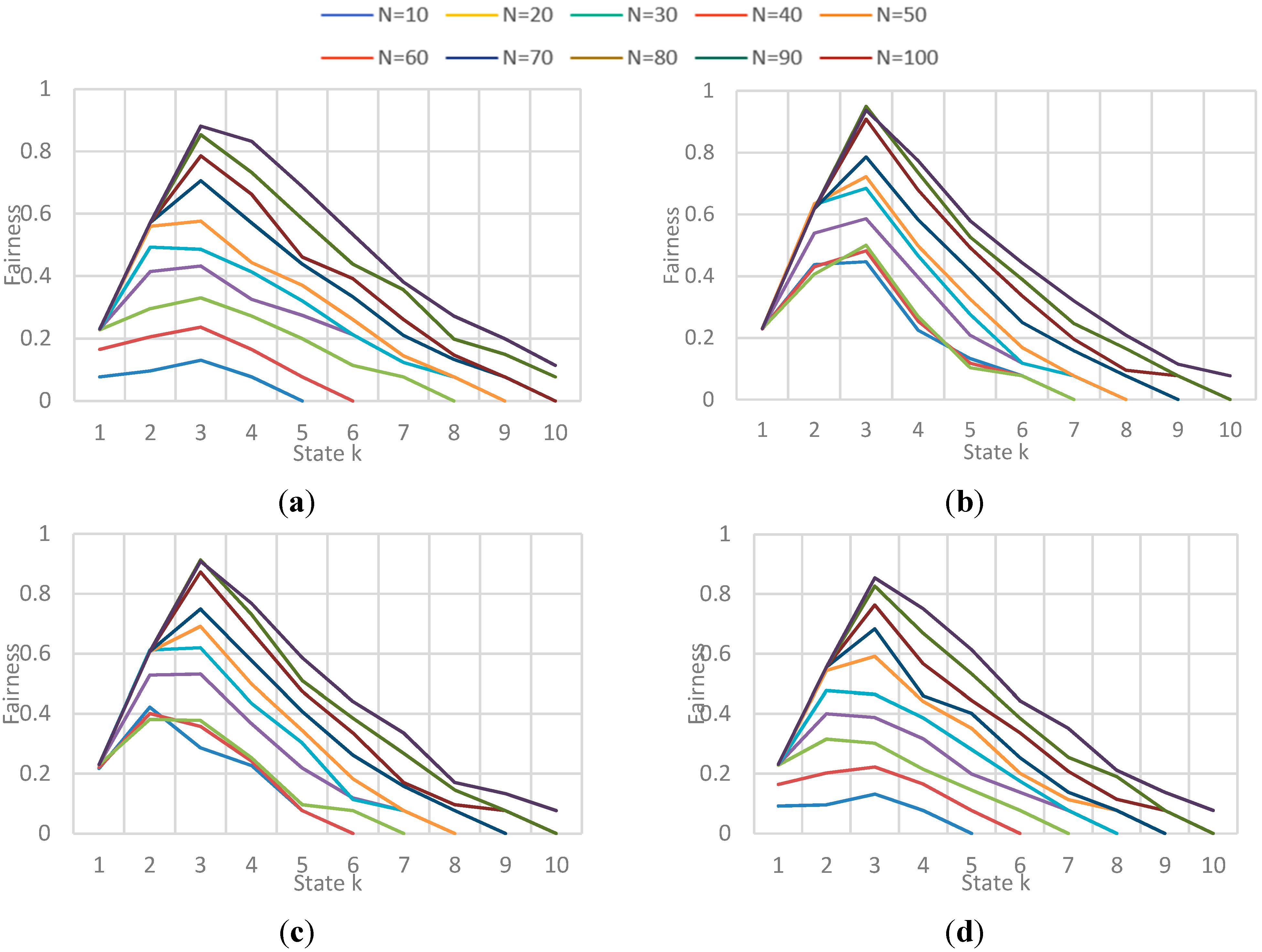
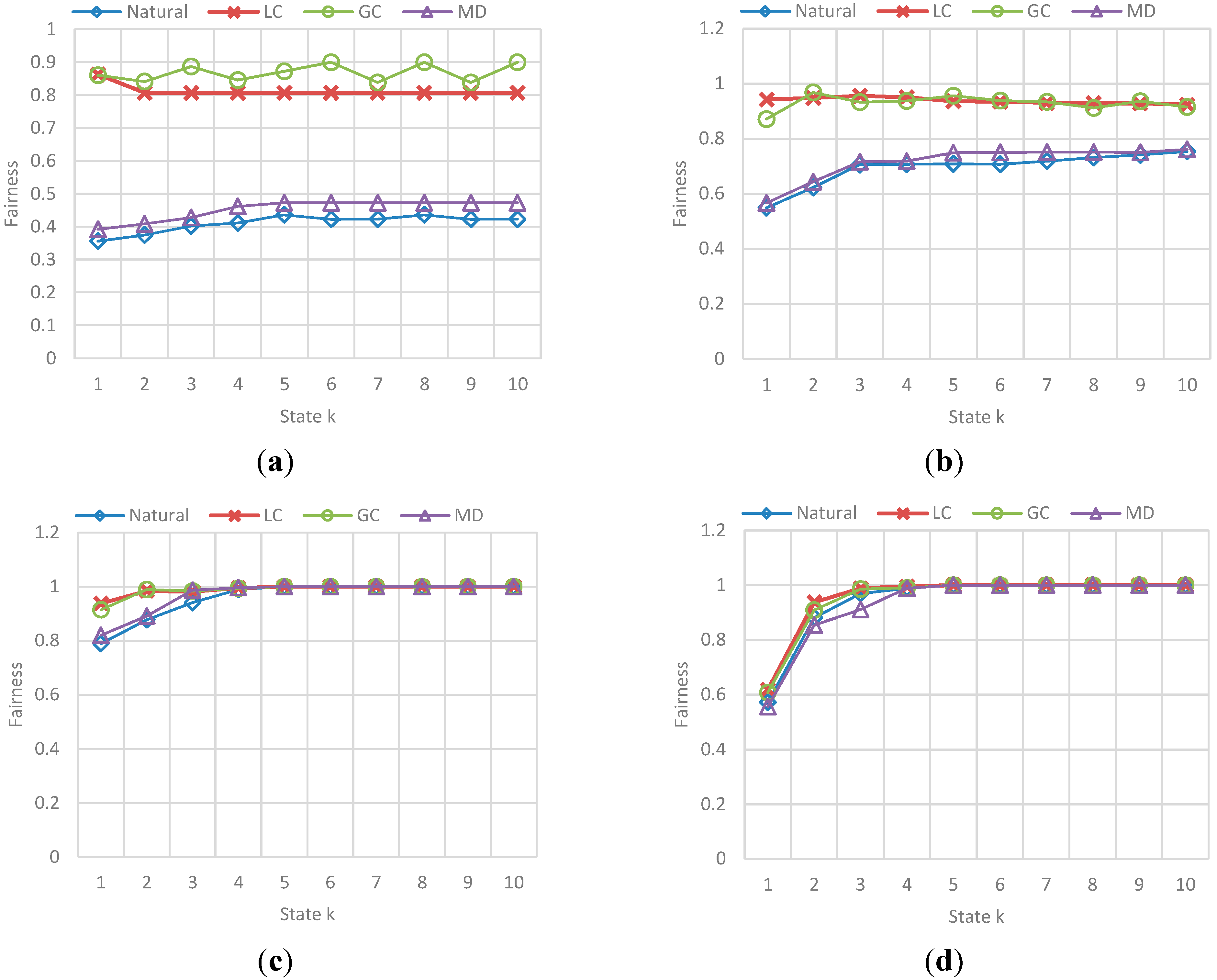
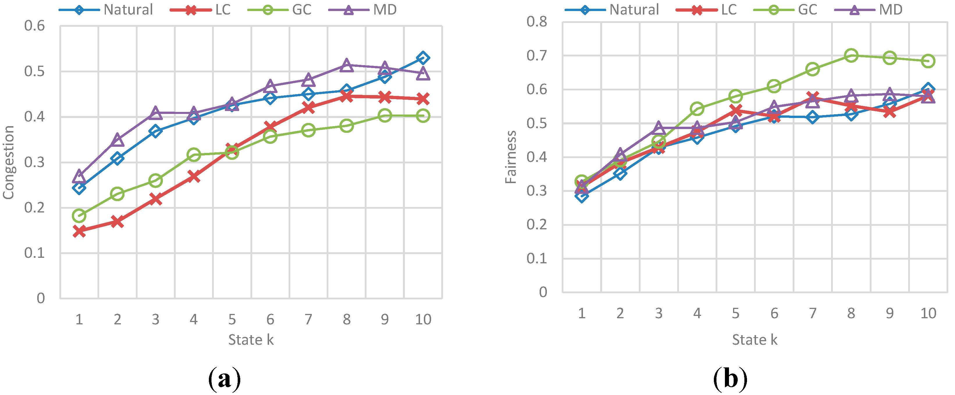
(b) Fairness and Congestion
- -
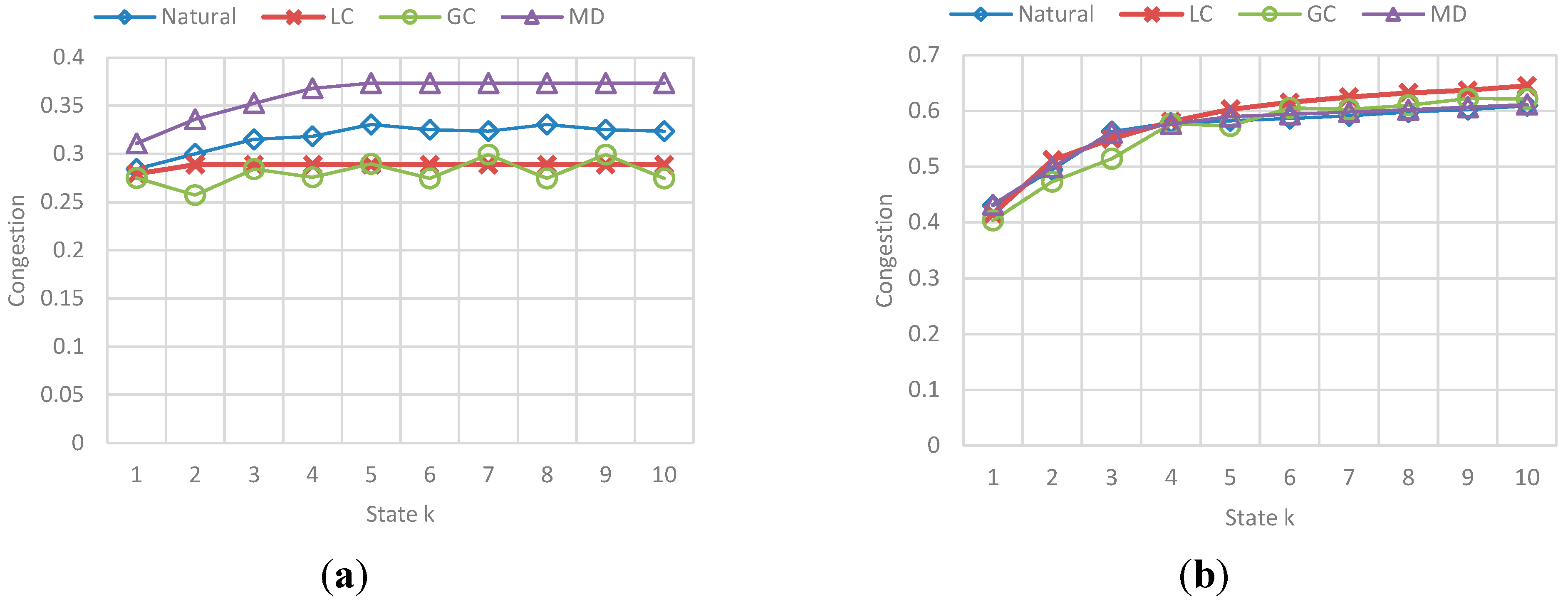
- Fairness behavior and congestion behavior are very similar: as the maximum capacity of the streets is reached, the streets get saturated which result in a high congestion level implying that the use percentage of the streets is very similar.
- -
- GC and LC implementations obtain the highest values in fairness when the congestion level is not high, that means the streets are being used better in those cases. Also, those implementations obtained the best values in efficiency, showing that exists a relation between the trip efficiency for each vehicle, and the use balance in the streets.

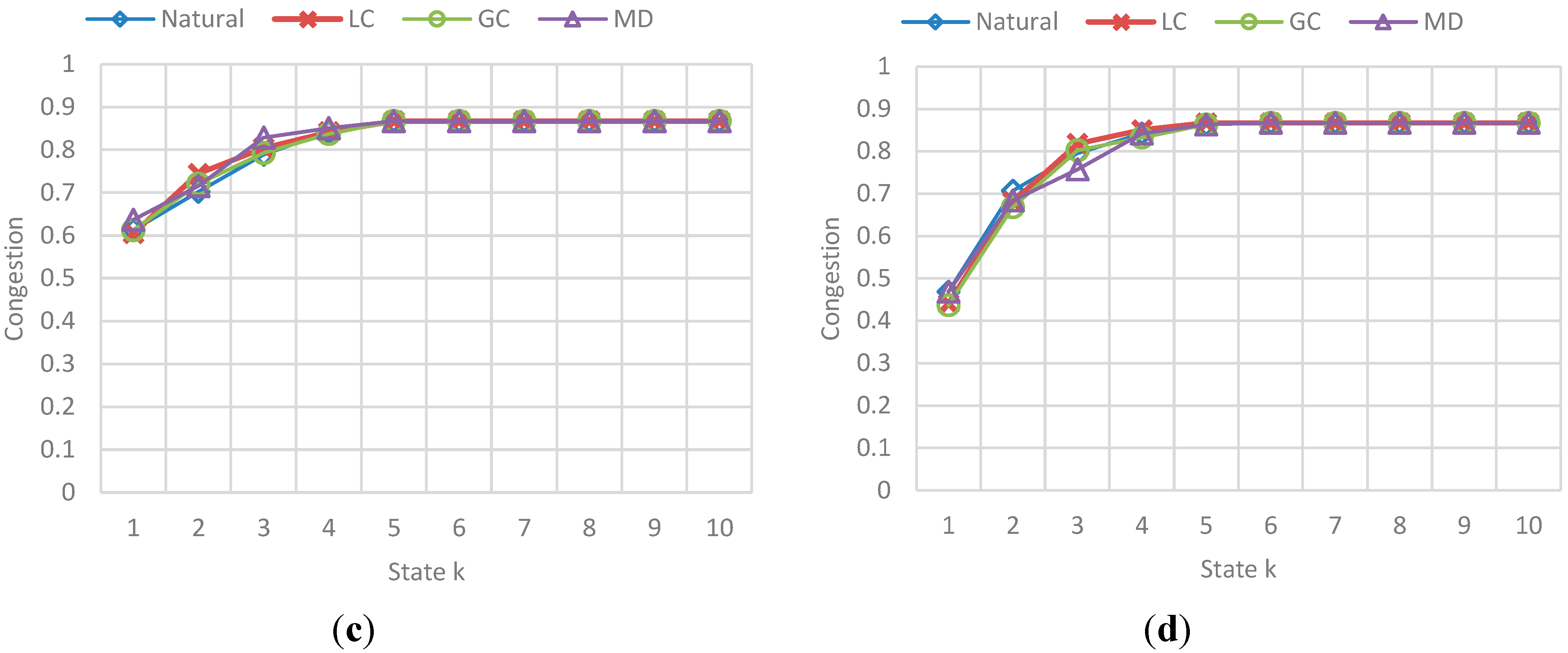
6.2.2. F Vehicles
(a) Efficiency and Distance


- -
- As the number F of vehicles increases, simulation results for efficiency in the previous simulation are replicated: the route efficiency in all implementations decreases as the set of vehicles in the network reaches the saturation value, in fact, for F = 30 and F = 40 there is not a great difference between efficiency values in the implementations.
- -
- In addition, even when the efficiency values are similar GC have better results. In ontrast, this implementation have one of the worst trip distance value.
- -
- Trip distance is again related with the efficiency showing a similar increasing/decreasing behavior compared with the efficiency behavior.
(b) Fairness and Congestion


- -
- As the previous simulation, the GC and LC fairness is much better than Normal and SMD in low congestion levels of the network, while in high levels of congestion the fairness is pretty much the same. In addition, a relation between fairness and route efficiency exists.
6.3. Reference Scenario Results
- -
- It is appreciated that for GC, efficiency is more stable with the best results among the other implementations. Nevertheless, we can see again that the GC implementation that provides better efficiency is one of the implementation that has a greater distance, and the distance to DT usually better.
- -
- Additionally, the average congestion in the simulation was not very big and the fairness values for implementations are very similar, however, GC has a better Fairness when the levels of congestion are no over the limit.
- -
- For the Normal implementation, efficiency values are low (up to 60%–70% worse compared with the best value) and distance is not the best, so this implementation really does not offer any advantage over the others.
7. Conclusions
Acknowledgments
Author Contributions
Conflicts of Interest
References
- Chen, L.W.; Sharma, P.; Tseng, Y.C. Dynamic Traffic Control with Fairness and Throughput Optimization Using Vehicular Communications. IEEE J. Sel. Areas Commun. 2013, 31, 504–512. [Google Scholar] [CrossRef]
- Agudelo, J.; Castro Barrera, H. Approach for a Congestion Charges System Supported on Internet of Things. In Proceedings of the 2014 IEEE Colombian Conference on Communications and Computing (COLCOM), Bogotá, Colombia, 4–6 June 2014; pp. 1–6.
- Información Pico y Placa en Colombia. Available online: http://www.picoyplaca.info/ (accessed on 20 October 2014).
- U.S. Department of Transportation. Research and Innovative Technology Administration. Available online: http://www.itsoverview.its.dot.gov/ (accessed on 8 April 2014).
- Rafiq, G.; Talha, B.; Patzold, M.; Gato Luis, J.; Ripa, G.; Carreras, I.; Coviello, C.; Marzorati, S.; Perez Rodriguez, G.; Herrero, G.; et al. What’s New in Intelligent Transportation Systems?: An Overview of European Projects and Initiatives. IEEE Veh. Technol. Mag. 2013, 8, 45–69. [Google Scholar] [CrossRef]
- Wedel, J.; Schunemann, B.; Radusch, I. V2X-Based Traffic Congestion Recognition and Avoidance. In Proceedings of the 2009 10th International Symposium on Pervasive Systems, Algorithms, and Networks (ISPAN), Kaohsiung, Taiwan, 14–16 December 2009; pp. 637–641.
- Dijkstra, E.W. A note on two problems in connexion with graphs. Numer. Math. 1959, 1, 269–271. [Google Scholar] [CrossRef]
- Nha, V.T.N.; Djahel, S.; Murphy, J. A comparative study of vehicles’ routing algorithms for route planning in smart cities. In Proceedings of the 2012 1st International Workshop on Vehicular Traffic Management for Smart Cities, Dublin, UK, 20 November 2012.
- Fontanelli, S.; Bini, E.; Santi, P. Dynamic route planning in vehicular networks based on future travel estimation. In Proceedings of the 2010 IEEE Vehicular Networking Conference (VNC), Jersey, NJ, USA, 13–15 December 2010; pp. 126–133.
- Lakas, A.; Cheqfah, M. Detection and dissipation of road traffic congestion using vehicular communication. In Proceedings of the 2009 Mediterrannean Microwave Symposium (MMS), Tangier, Morocco, 15–17 November 2009; pp. 1–6.
- Kok, A.L.; Hans, E.W.; Schutten, J.M.J. Vehicle routing under time-dependent travel times: The impact of congestion avoidance. Comput. Oper. Res. 2012, 39, 910–918. [Google Scholar] [CrossRef]
- Sheng-Hai, A.; Lee, B.H.; Shin, D.R. A Survey of Intelligent Transportation Systems. In Proceedings of the 2011 Third International Conference on Computational Intelligence, Communication Systems and Networks (CICSyN), Bali, Indonesia, 26–28 July 2011; pp. 332–337.
- European Telecommunications Standards Institute (ETSI). Intelligent Transport Systems (ITS); Communications Architecture. 2010. Available online: http://webapp.etsi.org/workprogram/Report_WorkItem.asp?WKI_ID=28554 (accessed on 17 October 2014).
- ISO/IEC 7498-1. Information technology—Open Systems Interconnection–Basic Reference Model: The Basic Model. 1994. Available online: http://www.ecma-international.org/activities/Communications/TG11/s020269e.pdf (accessed on 17 October 2014).
- Perera, C.; Zaslavsky, A.; Christen, P.; Georgakopoulos, D. Context Aware Computing for The Internet of Things: A Survey. IEEE Commun. Surv. Tutor. 2014, 16, 414–454. [Google Scholar] [CrossRef]
- Cunha, F.D.; Boukerche, A.; Villas, L. Data Communication in VANETs: A Survey, Challenges and Applications. Available online: https://hal.inria.fr/hal-00981126/document (accessed on 17 October 2014).
- Jiang, D.; Delgrossi, L. IEEE 802.11p: Towards an International Standard for Wireless Access in Vehicular Environments. In Proceedings of the IEEE Vehicular Technology Conference (VTC Spring 2008), Singapore, 11–14 May 2008; pp. 2036–2040.
- Chou, C.M.; Li, C.Y.; Chien, W.M.; Chan Lan, K. A Feasibility Study on Vehicle-to-Infrastructure Communication: WiFi vs. WiMAX. In Proceedings of the Tenth International Conference on Mobile Data Management: Systems, Services and Middleware (MDM’09), Taipei, Taiwan, 18–20 May 2009; pp. 397–398.
- Ibanez, A.; Flores, C.; Reyes, P.; Barba, A.; Reyes, A. A Performance Study of the 802.11p Standard for Vehicular Applications. In Proceedings of the 2011 7th International Conference on Intelligent Environments (IE), Nottingham, England, 25–28 July 2011; pp. 165–170.
- Jansons, J.; Petersons, E.; Bogdanovs, N. Vehicle-to-infrastructure communication based on 802.11n wireless local area network technology. In Proceedings of the 2012 2nd Baltic Congress on Future Internet Communications (BCFIC), Vilnius, Lithuania, 25–27 April 2012; pp. 26–31.
- Bazzi, A.; Masini, B. Taking advantage of V2V communications for traffic management. In Proceedings of the 2011 IEEE Intelligent Vehicles Symposium (IV), Baden-Baden, Germany, 5–9 June; pp. 504–509.
- Kihl, M.; Bur, K.; Mahanta, P.; Coelingh, E. 3GPP LTE downlink scheduling strategies in vehicle-to-infrastructure communications for traffic safety applications. In Proceedings of the 2012 IEEE Symposium on Computers and Communications (ISCC), Cappadocia, Turkey, 1–4 July 2012; pp. 000448–000453.
- Vinel, A. 3GPP LTE Versus IEEE 802.11p/WAVE: Which Technology is Able to Support Cooperative Vehicular Safety Applications? IEEE Wirel. Commun. Lett. 2012, 1, 125–128. [Google Scholar] [CrossRef]
- Imadali, S.; Kaiser, A.; Decremps, S.; Petrescu, A.; Veque, V. V2V2I: Extended inter-vehicles to infrastructure communication paradigm. In Proceedings of the Global Information Infrastructure Symposium, Trento, Italy, 28–31 October 2013; pp. 1–3.
- Zhan, F.B.; Noon, C.E. Shortest Path Algorithms: An Evaluation Using Real Road Networks. Transp. Sci. 1998, 32, 65–73. [Google Scholar] [CrossRef]
- Cao, L.; Shi, Z.; Bao, P. Self-adaptive Length Genetic Algorithm for Urban Rerouting Problem. In Advances in Natural Computation; Jiao, L., Wang, L., Gao, X.B., Liu, J., Wu, F., Eds.; Lecture Notes in Computer Science; Springer: Berlin/Heidelberg, Germany, 2006; Volume 4221, pp. 726–729. [Google Scholar]
- Dorigo, M.; Stützle, T. Ant Colony Optimization; MIT Press: Cambridge, MA, USA, 2004; pp. 1–16. [Google Scholar]
- Glover, F.; Laguna, M. Tabu Search. J. Comput. Biol. A J. Comput. Mol. Cell Biol. 1997, 16, 1689–1703. [Google Scholar]
- Kanoh, H.; Hara, K. Hybrid genetic algorithm for dynamic multi-objective route planning with predicted traffic in a real-world road network. In Proceedings of the Annual Conference on Genetic and Evolutionary Computation (GECCO), Atlanta, GA, USA, 12–16 July 2008; pp. 657–664.
- Wang, S.; Djahel, S; McManis, J.; McKenna, C.; Murphy, L. Proceedings of the Comprehensive Performance Analysis and Comparison of Vehicles Routing Algorithms in Smart Cities (IEEE GIIS 2013), Trento, Italy, 28–31 October 2013.
- Behrisch, M.; Bieker, L; Erdmann, J.; Krajzewicz, D. SUMO–Simulation of Urban Mobility—An Overview. In Proceedings of the Third International Conference on Advances in System Simulation, Barcelona, Spain, 23–28 October 2011.
- Donoso, Y.; Fabregat, R.; Marzo, J. A Multi-Objective Optimization Scheme for Multicast Routing: A Multitree Approach. Telecommun. Syst. 2004, 27, 229–251. [Google Scholar] [CrossRef]
- Donoso, Y.; Camelo, M.; Vila, P.; Lozano-garzon, C. A Fairness Load Balancing Algorithm in HWN Using a Multihoming Strategy Related Work. Available online: http://univagora.ro/jour/index.php/ijccc/article/view/1275 (accessed on 30 April 2014).
- Jain, R.; Chiu, D.; Hawe, W. A Quantitative Measure of Fairness and Discrimination for Resource Allocation in Shared Computer Systems. 1984. Available online: http://www.cse.wustl.edu/~jain/papers/fairness.htm (accessed on 30 April 2014).
- Wang, S.; Djahel, S; McManis, J. A Multi-Agent based vehicles re-routing system for unexpected traffic congestion avoidance. In Proceedings of the 17th International IEEE Conference on Intelligent Transportation Systems (IEEE ITSC 2014), Qingdao, China, 8–11 October 2014.
- Ministerio de Transporte de Colombia. Codigo de Tránsito de Colombia. Available online: http://www.colombia.com/noticias/codigotransito/ (accessed on 2 September 2014).
© 2015 by the authors; licensee MDPI, Basel, Switzerland. This article is an open access article distributed under the terms and conditions of the Creative Commons Attribution license (http://creativecommons.org/licenses/by/4.0/).
Share and Cite
Parrado, N.; Donoso, Y. Congestion Based Mechanism for Route Discovery in a V2I-V2V System Applying Smart Devices and IoT. Sensors 2015, 15, 7768-7806. https://doi.org/10.3390/s150407768
Parrado N, Donoso Y. Congestion Based Mechanism for Route Discovery in a V2I-V2V System Applying Smart Devices and IoT. Sensors. 2015; 15(4):7768-7806. https://doi.org/10.3390/s150407768
Chicago/Turabian StyleParrado, Natalia, and Yezid Donoso. 2015. "Congestion Based Mechanism for Route Discovery in a V2I-V2V System Applying Smart Devices and IoT" Sensors 15, no. 4: 7768-7806. https://doi.org/10.3390/s150407768